Masters Dissertation OPTIMIZATION OF 4G CELLULAR NETWORKS FOR THE REDUCTION OF ENERGY CONSUMPTION Samir Kolawolé Akanni Landou

i

Masters Dissertation

OPTIMIZATION OF 4G CELLULAR NETWORKS FOR THE

REDUCTION OF ENERGY CONSUMPTION

Samir Kolawolé Akanni Landou

Brasilia, August 2015

ii

UNIVERSITY OF BRASILIA

Faculty of Technology

MASTERS DISSERTATION

OPTIMIZATION OF 4G CELLULAR NETWORKS FOR THE

REDUCTION OF ENERGY CONSUMPTION

Samir Kolawolé Akanni Landou

A thesis submitted to the University of Brasilia

in partial fulfillment of the requirements for the

degree of Master in Electrical Engineering

Program of Study Committee:

Prof. André Noll Barreto, ENE/UnB ____________________________________ Advisor

Prof. Vicente Angelo de Sousa Junior, UFRN _____________________________________ External examiner

Prof. Leonardo Aguayo, FGA/UnB _____________________________________

Internal examiner

iii

DATA CATALOG

BIBLIOGRAPHIC REFERENCE

S. K. A. LANDOU (2015). Optimization of 4G Cellular Networks for the Reduction of Energy

Consumption. A thesis submitted in partial fulfillment of the requirements for the degree of

Master in Electrical Engineering, Publication PPGEE.DM-606/2015, Department of Electrical Engineering, University of Brasilia, Brasilia, DF, 54p.

ASSIGNMENT OF RIGHTS

AUTHOR: Samir Kolawolé Akanni Landou

TITLE: Optimization of 4G Cellular Networks for the Reduction of Energy Consumption. GRADE: Master degree

YEAR: 2015

It is granted to the University of Brasilia permission to reproduce copies of this work and to lend or sell such copies only for academic and scientific purposes. The author reserve other rights of publication and no part of this course conclusion work may be reproduced without written permission of the author.

Samir Kolawolé Akanni Landou

Campus Universitário Darcy Ribeiro, Asa Norte CEP: 70.910-900 Brasília – DF – Brazil

SAMIR KOLAWOLÉ AKANNI LANDOU

Optimization of 4G Cellular Networks for the Reduction of Energy Consumption [Distrito Federal] 2015.

xv, 54p., 210 x 297 mm (ENE/FT/UnB, Master, Electrical Engineering). A thesis submitted to the University of Brasilia in partial fulfillment of the requirements for the degree of Master in Electrical Engineering.

1. Cell zooming 2. CoMP

3. Coordinated Multipoint 4. Energy efficiency 5. Green Cellular Networks 6. Sleep mode.

iv

ACKNOWLEDGEMENTS

I would like to take this opportunity to appreciate my advisor Professor Dr. André Noll Barreto. Without whom, I would not have gotten the opportunity to study in the University of Brasilia and have new experience in this wonderful country. His tolerance and understanding helped me to endure the hard times and to overcome any possible difficulty to carry out this project.

I am thankful to CAPES for giving me the financial support without which I could not have kept myself in Brazil and complete this project.

I am thankful to my family and my girlfriend for their love, support and encouragement throughout this work.

Finally, I would like to thank my friends and colleagues for their help and motivations throughout this work.

v

ABSTRACT

With the growth of cellular networks and emergence of new technologies, the power consumption and energy efficiency of cellular networks have become more important. Recently, green communications have received much attention in order to reduce the energy consumption and minimize the carbon dioxide (CO2) emission. In this work, we are interested in power efficiency methods which optimize the energy saving of the cellular networks especially altering the transmitted power of base stations. We investigate some solutions found in the literature, namely sleep mode and cell zooming techniques. We also investigate the use of Coordinated Multi-Point (CoMP) transmission radio technology in order to improve the quality of the network.

Keywords: Cell zooming, CoMP, Coordinated Multipoint, Energy efficiency, Green Cellular

vi

RESUMO

Com o crescimento das redes celulares e com o surgimento de novas tecnologias, o consumo de energia e a eficiência energética das redes celulares se tornaram mais importantes. Recentemente, as comunicações verdes têm recebido muita atenção, a fim de reduzir o consumo de energia e minimizar as emissões de dióxido de carbono (CO2). Neste trabalho, estamos interessados em métodos de eficiência energética que otimizam a redução do consumo de energia das redes celulares, especialmente alterando a potência transmitida de estações de base. Investigamos algumas soluções encontradas na literatura, a saber, o sleep mode e o cell zooming. Nós investigamos também o uso do Coordinated Multi-Point (CoMP), uma tecnologia de rádio de transmissão coordenada, a fim de melhorar a qualidade da rede.

Palavras-chave: Cell zooming, CoMP, Coordinated Multipoint, Energy efficiency, Green

vii

RESUMÉ

Avec la croissance des réseaux cellulaires et l'émergence de nouvelles technologies, la consommation d'énergie et l'efficacité énergétique des réseaux cellulaires sont devenues plus importantes. Récemment, les communications vertes ont reçu beaucoup d'attention dans le but de réduire la consommation d'énergie et de réduire les émissions de dioxyde de carbone (CO2). Dans ce travail, nous nous intéressons à des méthodes d'efficacité de puissance qui optimisent l’économie d'énergie des réseaux cellulaires en altérant particulièrement la puissance transmise des stations de base. Nous avons étudié des solutions trouvées dans la littérature, à savoir le

sleep mode et le cell zooming. Nous avons étudié également l'utilisation de Coordinated

Multi-Point (COMP), une technologie de radio de transmission coordonnée, afin d'améliorer la qualité

du réseau.

Mots-clés: Cell zooming, CoMP, Coordinated Multipoint, Energy efficiency, Green Cellular

viii

TABLE OF CONTENTS

1. INTRODUCTION ... 1

1.1 - BACKGROUND ... 1

1.2 - OBJECTIVE ... 2

1.3 - TOOLS ... 3

1.4 - DISSERTATION LAYOUT ... 3

2. CELLULAR NETWORKS ... 4

2.1 - EVOLUTION OF CELLULAR NETWORKS ... 4

2.2 - BASIC CONCEPTS OF A CELLULAR NETWORK ... 6

2.2.1 - Mobility of UE in cellular network ... 7

2.2.2 - The Radio Access Network ... 7

2.2.3 - The Core Network... 8

3. GREEN CELLULAR NETWORKS ... 9

3.1 - METRICS FOR CELLULAR NETWORKS ... 11

3.2 - BS ARCHITECTURAL CHANGES ... 12

3.2.1 - Cell zooming ... 12

3.2.2 - Sleep mode ... 13

3.3 - COORDINATED MULTI-POINT (CoMP) ... 14

4. SYSTEM MODELING (SIMULATOR) ... 17

4.1 - BASIC ENVIRONMENT ... 18

4.1.1 - Cell grid ... 19

4.1.2 - Hotspots ... 19

4.1.3 - Base stations... 20

4.1.4 - Traffic ... 21

4.1.5 - User mobility ... 22

4.1.6 - Channel model ... 22

4.1.7 - Link model ... 25

4.2 - CENTRALIZED SERVER ... 27

4.3 - PARAMETERS ... 27

ix

5. SIMULATION SCENARIOS ... 30

5.1 - PREVIOUS WORK ... 30

5.1.1 - Standard mode ... 30

5.1.2 - Classical cell zooming ... 31

5.1.3 - Sleep mode ... 32

5.2 - CoMP ... 34

5.3 - SCENARIOS ... 35

5.4 - SIMULATION RESULTS ... 37

5.4.1 - Scenario 1: Standard mode ... 37

5.4.2 - Scenario 2: Classical cell zooming ... 39

5.4.3 - Scenario 3: Sleep mode ... 41

5.4.4 - Scenario 4: Classical cell zooming + CoMP ... 45

5.4.5 - Scenario 5: Sleep mode + CoMP ... 47

5.5 - ANALYSES AND DISCUSSION ... 50

6. CONCLUSION ... 51

x

LIST OF FIGURES

Figure 1.1 - Cellular network power consumption (from [2]). ... 1

Figure 1.2 - Mobile broadband coverage reach, 2009-2020 (from [5]) ... 3

Figure 2.1 - A summary of wireless technologies evolution since 2G (from [15]). ... 6

Figure 2.2 - Cellular network structure (adapted from [12]). ... 6

Figure 2.3 - Frequency reuse pattern with factor 1:7 (from [16]). ... 7

Figure 2.4 - Directive Antenna in a tri-sectored cell in a cell grid (from [11]). ... 8

Figure 3.1 - Cell zooming concepts (adapted from [7]). ... 12

Figure 3.2 - Sleep mode concepts (adapted from [7]). ... 13

Figure 3.3 - Coordinated Scheduling/Beamforming concept (adapted from [8]). ... 14

Figure 3.4 - Coordinated Dynamic Cell Selection concept (adapted from [4]). ... 15

Figure 3.5 - Coordinated Joint Transmission concept (adapted from [8]). ... 16

Figure 3.6 - Illustration of intra-site and inter-site CoMP (from [22]). ... 16

Figure 4.1 - Relation between each class of the simulator (From [11]). ... 18

Figure 4.2 - Hexagonal cells grid (from [11]). ... 19

Figure 4.3 - Power consumption distribution in a BS (Adapted from [3]). ... 21

Figure 4.4 - Traffic model (adapted from [17]). ... 21

Figure 4.5 - Example of grid for the estimation of the SF (adapted from [25]). ... 24

Figure 4.6 - LTE downlink resources (from [26]). ... 26

Figure 5.1 - Rectangular grid of hexagonal cells and its configuration in the execution of the sleep mode (adapted from [18]). ... 33

Figure 5.2 - Flowchart of the mains steps of the simulation scenarios ... 36

Figure 5.3 - Traffic profile during a day. ... 37

Figure 5.4 - UE downlink throughput. ... 38

Figure 5.5 - Outage probability. ... 38

Figure 5.6 - Consumed power per BS. ... 39

Figure 5.7 - Consumed power per BS in scenario 2. ... 39

Figure 5.8 - UE downlink throughput in scenario 2. ... 40

Figure 5.9 - Outage probability in scenario 2. ... 40

Figure 5.10 - Consumed power per BS in scenario 3. ... 41

Figure 5.11 - Consumed power: 75% sleep mode with different values of server granularity. 41 Figure 5.12 - Consumed power: 50% Sleep mode with different values of server granularity. 42 Figure 5.13 - Consumed power: 25% Sleep mode with different values of server granularity. 42 Figure 5.14 - Consumed power with different condition of sleep mode activation. ... 43

Figure 5.15 - UE downlink throughput with different condition of sleep mode activation. ... 43

Figure 5.16 - Outage Probability with different condition of sleep mode activation. ... 44

Figure 5.17 - UE downlink throughput in scenario 3. ... 44

Figure 5.18 - Outage probability (with different sleep mode schemes) in scenario 3. ... 45

Figure 5.19 - Consumed power per BS in scenario 4. ... 45

Figure 5.20 - UE downlink throughput in scenario 4. ... 46

xi

Figure 5.22 - UE CoMP usage ratio in scenario 4. ... 47

Figure 5.23 - Consumed power per BS in scenario 5. ... 47

Figure 5.24 - UE downlink throughput in scenario 5. ... 48

Figure 5.25 - Outage probability in scenario 5. ... 48

xii

LIST OF TABLES

Table 3.1 - Techniques used for a green cellular networks. ... 10

Table 3.2 - Metrics for cellular networks. ... 11

Table 3.3 - Classical cell zooming scenarios. ... 13

Table 3.4 - Sleep mode scenarios. ... 14

Table 4.1 - Hotspots specifications (adapted from [18]). ... 19

Table 4.2 - UEs mobility specifications (adapted from [18]). ... 22

Table 4.3 - Shadowing factor values (adapted from [25]). ... 24

Table 4.4 - Parameters of the LTE downlink structure (Adapted from [26]). ... 26

Table 4.5 - Simulator parameters (adapted from [11]). ... 27

Table 5.1 - Classical cell zooming system parameters. ... 31

Table 5.2 - Condition for Classical cell zooming execution. ... 31

Table 5.3 - Examples of sleep mode denomination ... 32

Table 5.4 - Sleep mode system parameters. ... 33

Table 5.5 - CoMP system parameters. ... 34

xiii

LIST OF ABBREVIATIONS

1G 1st Generation of cellular networks

2G 2nd Generation of cellular networks

3G 3rd Generation of cellular networks

3GPP 3rd Generation Partnership Project

4G 4th Generation of cellular networks

1xEVDO 1x Evolution Data Optimized

AMPS Advanced Mobile Phone System

AU Antenna Unit

AUC Authentication Center

AWGN Additive White Gaussian Noise

BPSK Binary Phase Shift Keying

BS Base Station

CB Coordinated Beamforming

C-NETZ Funktelefonnetz-C

CDMA Code-Division Multiple Access

CN Core Network

CoMP Coordinated Multi-Point

CP Cyclic Prefix

CS Coordinated Scheduling

DCS Dynamic Cell Selection

DL Downlink

EDGE Enhanced Data rates for GSM Evolution

ETSI European Telecommunications Standards Institute

FDMA Frequency-Division Multiple Access

GPRS General Packet Radio Service

xiv HLR home location register

HSPA High Speed Packet Access

ICI Inter-cell Interference

IP Internet Protocol

IS-95 Interim Standard 95

JP Joint Processing

JT Joint Transmission

LOS Line-of-Sight

LTE Long Term Evolution

LTE-A LTE-Advanced

MMS Multimedia Message Service

MU Mobile User

MSC Mobile Switching Centers

NLOS Non Line-of-Sight

NMT Nordic Mobile Telephone

OFDM Orthogonal Frequency-Division Multiplexing

OSS Operation and Support Systems

PDN Packet Data Network

PL Path Loss

PSTN Public Switched Telephone Network

PV Photovoltaic

QAM Quadrature Amplitude Modulation

QoE Quality of Experience

QoS Quality of Service

QPSK Quadrature Phase Shift Keying

RAN Radio Access Network

RB Resource Block

xv SF Shadowing Factor

SIM Subscriber Identity Module

SNIR Signal-Interference-to-Noise-Ratio

SMS Short Message Service

SMSC Short Message Service Centers

TACS Total Access Communication System

TDMA Time-Division Multiple Access

UE User Equipment

UL Uplink

UMTS Universal Mobile Telecommunication Service

VLR Visitor Location Register

VoIP Voice over Internet Protocol

1

1.

INTRODUCTION

1.1 - BACKGROUND

Within twenty years, the use of mobile communication services has grown considerably. The wireless network has become today a communication system essential for society. 3GPP-LTE (Long Term Evolution) is the latest standard technology of cellular networks that paved the way for a new generation of mobile radio, marketed by operators as the fourth generation (4G).

Standardized by 3GPP (3rd Generation Partnership Project), which is a mobile radio standardization forum, LTE enabled considerable improvement in the quality of service (QoS) of mobile systems, and the quality of experience (QoE) of users, when compared with the previous generations of cellular networks.

However, with the rapid evolution of cellular networks in the world, one should take into account the issue of energy efficiency, since telecommunication industries are responsible for about 2 percent of the total CO2 emissions in the world and this number is predicted to double

by 2020 with the exponential growth of mobile traffic [1]. The increase in energy consumption is caused by the growing number of user equipments (UEs), the subscription to higher rates of mobile broadband data, as well as the higher contribution of information technology in the world [2].

This increase has an environmental impact in the world, not to mention economic. This fact has been gaining importance lately, especially with wireless networks [3]. In particular, solutions should be focused on the architecture and system design techniques of mobile cellular networks, particularly in the base stations (BS), which contribute 60 to 80 % (Figure 1.1) of the total energy consumed in the network [4].

This concept of reducing energy consumption is known as “Green Cellular Networks”.

2 1.2 - OBJECTIVE

Nowadays, LTE 4th generation (4G) technology is implemented in most countries of the world and is still rapidly expanding in several countries which are still under 3rd generation (3G) technology (Figure 1.2); in other words, more than four out of five people worldwide will have access to 3G networks by 2020 (up from 70% nowadays), while 4G networks will cover 60% of the global population by this point (up from 25% nowadays) [5]. It is foreseeable that global population in a near future will be covered by 4G technology, which is becoming the worldwide dominant cellular networks technology in the world.

However, cellular networks essentially operate in 24 hours a day “always on”, and base stations in particular consume significant power even when not carrying traffic [6]. Unfortunately, energy consumption has become one of the most important issues in the world, as the carbon emissions of energy sources have great negative impact on the environment, and the price of energy is also increasing [7].

Hence, it is of particular interest to investigate the green concept for LTE (4G) technology in order to reduce carbon footprint in the world.

Consequently, we investigate in this work some techniques suggested in the literatures. One of them is cell zooming, which consists in adjusting the cell size according to traffic condition [1] through antenna tilts and variable transmission power. Another one is the sleep mode approach, where some base stations (BS) can be switched off when their traffic loads are below a certain threshold for a certain period of time [8], thus reducing the number of active BSs. However, sleep mode and cell zooming techniques may result in coverage holes and higher outage probabilities while reducing the power consumption.

The goal of this work is to investigate solutions that not only reduce the energy consumption, but also maintain the quality of the network.

Thus, to overcome the problem of energy consumption growth and higher outage probabilities due to coverage holes, we extend in particular the concept of cell zooming and sleep mode by the use of Coordinated Multi-Point (CoMP), which is one of the techniques currently proposed in 3GPP-LTE Release 11 [9].

In CoMP radio technology, neighboring BSs cooperate to transmit or receive the same information to/from some individual UEs. This technique is especially beneficial to UEs located at the cell edge [8].

3

Figure 1.2 - Mobile broadband coverage reach, 2009-2020 (from [5])

1.3 - TOOLS

To get results and conclusions related to our proposed scheme for a green cellular network, we improved a simulator which models the downlink of an LTE standard cellular network. This simulator, written in C++, has been built in a previous work (in [11]) to model long-term variation of UEs traffic, to measure the energy consumption and the downlink throughput of cellular networks.

In this work, we improve the simulator algorithm in order to reduce its execution time; to insert additional statistic data collection parameters; to modify the throughput calculation with Shannon’s capacity, to model the impact of channel coding; to insert CoMP algorithm and to simulate CoMP with sleep mode or cell zooming techniques in order to improve the energy efficiency.

Then, to analyze the results, graphs are generated to analyze the impact of a green communication on the network performance and the energy consumption of a cellular network before its real implementation. The source code of the simulator is freely available from the address https://sourceforge.net/projects/green-cellular-network .

1.4 - DISSERTATION LAYOUT

This dissertation report consists of six chapters. The chapters are organized as follows:

4

2.

CELLULAR NETWORKS

A cellular network is a technology which is designed for mobile communication. It allows UEs to communicate via radio interface. Originally created to provide only analog speech service, mobile communications technology has grown considerably with advanced technology; now, it allows access to data services (SMS (Short Message Service), MMS (Multimedia Message Service), Internet access, VoIP (Voice over Internet Protocol), etc.) to its subscribers.

This chapter presents the major evolution and the basic concepts of cellular network.

2.1 - EVOLUTION OF CELLULAR NETWORKS

The 1st _{generation (1G) of cellular Network was launched and commercialized at the first time,}

in the 1980s. Several technologies of cellular networks have been created such as:

- AMPS (Advanced Mobile Phone System) in United State of America,

- TACS (Total Access Communication System) in Japan and United Kingdom,

- RadioCom2000 in France,

- NMT (Nordic Mobile Telephone) in Scandinavia,

- C-NETZ (Funktelefonnetz-C) in Germany.

In 1G, only analog speech service was provided for UEs with a very limited system capacity of the system, and no compatibility among different systems. This capacity constraint as well as the high cost of mobile terminals and communication prices had restricted the use of 1G to limited number of UEs [12].

After 1G systems were deployed, much progress has been made, particularly in advanced radio mobile technologies, and new generations of cellular networks were born in order to improve the 1G’s drawbacks. In the 2nd _{Generation (2G), four cellular network technologies were}

created:

- GSM (Global System Mobile communications) in Europe,

- PDC (Personal Digital Communications) in Japan,

- IS-95 (Interim Standard 95) in USA.

- IS-136 (TDMA) in USA.

These systems, in their original versions, gave access to voice service with mobility, and also allowed low-speed data transfers, and short text messages, best known as SMS (Short Message Service) [12].

5

IS-95 was based on CDMA (Code-Division Multiple Access), and provided access to multiple UEs on the same channel, each with a different spreading code, allowing great increase in network capacity.

GSM, which is still widely used, is based on FDMA (Frequency Division Multiple Access) and TDMA (Time Division Multiple Access). Two new standards were derived from GSM by ETSI (European Telecommunications Standards Institute) to incorporate the data packet switching to the already employed circuit switching: GPRS (General Packet Radio Service) and EDGE (Enhanced Data rates for GSM Evolution). The GSM / GPRS / EDGE family makes use of SIM (Subscriber Identity Module) cards and multiple access is based on time and frequency (TDMA / FDMA) [12], [13] for all versions.

However, at the end of the 1990s, data rates provided by 2G networks were still too limited to access data services fluidly. This limitation has been the motivation for the definition of the 3rd

Generation (3G) technologies, which are initially characterized by the will of the telecommunication industries to define a global standard. The goals were to offer global roaming to UEs, but also to reduce the unit costs of mobile terminals and network equipment.

The main technologies that have emerged in 3G are UMTS (Universal Mobile Telecommunications System) from GSM, and CDMA2000 from IS-95. Companies, particularly those from the GSM world, have gathered in a consortium called 3GPP (3rd Generation Partnership Project) to develop the UMTS standard in late the 1990s. The first version of the standard is called Release 99 [11]. The main difference between 3G systems and its predecessors is the larger data rate in the former [13].

HSPA (High Speed Packet Access) and HSPA+ (High Speed Packet Access+) are two technologies standardized after UMTS by 3GPP (Release 7), in order to improve UMTS’ performance bringing very significant benefits in terms of data rate, capacity and latency. UMTS met a greater commercial success than CDMA2000 and nowadays, it is widely deployed on every continent [12].

Since 1G, there was a great improvement in QoS, QoE and services provision (voice, data, multimedia, etc.). However, for a further improvement, a new technology was defined and standardized by 3GPP (Release 8) in December 2008 during the Future Evolution Workshop for the evolution in long term of UMTS. Thus, the name LTE (Long Term Evolution) has been defined by 3GPP for this technology considered as a fourth stage of the evolution of mobile access networks, also called commercially 4th _{Generation (4G).}

LTE has been standardized to achieve high peak rates in DL (Downlink) and UL (Uplink); to reduce latency; to improve spectral efficiency; to have a flexible bandwidth; to support mobility between different access networks (2G/3G); to implement a new simplified network architecture; and to ensure compatibility with earlier 3GPP Releases [14].

The evolution of LTE is called LTE-A (LTE-Advanced). It has been introduced since Release 10 by 3GPP in order to improve LTE technology.

6

Figure 2.1 - A summary of wireless technologies evolution since 2G (from [15]).

2.2 - BASIC CONCEPTS OF A CELLULAR NETWORK The architecture of a cellular network is based on three entities:

- the Mobile User (MU) or User Equipment (UE);

- the Radio Access Network (RAN);

- the Core Network (CN).

Figure 2.2 shows a simplified scheme of the cellular network structure.

Figure 2.2 - Cellular network structure (adapted from [12]). Radio Access

Network Core Network

UE

Radio Interface

Terrestrial Interface

7 2.2.1 - Mobility of UE in cellular network

Mobility is one of the key factors of wireless networks. It gives UEs freedom of movement. Depending on the radio technology, mobility can be either limited to pedestrian speeds only, or can support communication even at high speeds [16]. The two key concepts of mobility are roaming and handovers.

Roaming can be defined as the movement of a UE from one network to another while handover is the process of switching a call or session that is in progress from one physical channel to another [16].

2.2.2 - The Radio Access Network

The radio access network is the largest component of the mobile network, and a large number of base stations and cell sites are provisioned in order to provide coverage [16]. Mobile networks are based on the concept of cell; hence, the name Cellular Network. Cell size in an urban area is usually less than the one in a rural area. Cells are categorized in macrocell, microcell, picocell, and femtocell, depending on their radius and transmit power level. A cell is controlled by a transmitter/receiver called base station (BS) that provides the radio link with UEs in its coverage area. The coverage of a base station is limited by several factors including:

- the transmit power of UE and BS;

- the frequency used;

- the type of antennas used for BS and UE;

- the wave propagation in the environment (urban, rural, etc.);

- the radio technology used.

A cell is generally represented in the form of a hexagon which represents the geometric pattern of the coverage area that ensures a regular grid space. In reality, there are of course areas of overlap between adjacent cells that create inter-cell interference [12]. To minimize the inter-cell interference, a reuse frequency with a factor of reuse is commonly used. Figure 2.3 shows an example of frequency reuse with a factor 1:7.

8

Also, directive antennas are usually used to minimize the interference between neighboring BSs. They can be configured in sectors.

Figure 2.4 shows an example of directive antennas in a tri-sectored cell.

Figure 2.4 - Directive Antenna in a tri-sectored cell in a cell grid (from [11]).

2.2.3 - The Core Network

9

3.

GREEN CELLULAR NETWORKS

The notion of “green” technology in wireless systems can be made meaningful with a comprehensive evaluation of energy savings and performance in a practical system [3]. The concept of green cellular network is becoming a necessity to support social, environmental, and economic sustainability [8].

In some papers in the literature, several methods for energy saving in access networks are proposed by authors, implementing mostly cell size adjustment according to the traffic load fluctuations.

 N. Zhisheng, W. Yiqun, G. Jie and Y. Zexi [7] proposed a scheme where cells with low traffic zoom to zero and its neighboring cells zoom out with BS physical adjustments in order to compensate the coverage hole.

 X. Wang, P. Krishnamurthy and D. Tipper [6] studied the feasibility and benefits of “BS sleeping” for energy conservation.

 E. Oh et al [17] proposed an estimate of the potential base station energy saving based on real cellular traffic traces.

 T. Han and N. Ansari [8] proposed multicell cooperation solutions for improving the energy efficiency of cellular networks. The authors categorized it into three solutions i.e. sleep mode, renewable energy, and CoMP.

 B. S. Carminati, M. F. Costa and A. N. Barreto [18] focused the study of energy efficiency through power management using sleep mode and virtual cell zooming. Our work is a continuation of the system modeling presented by B. S. Carminiti et al.

 S. Tombaz, A. Västberg and J. Zander [19] proposed a framework for a total cost analysis and surveyed some strategies to minimize the overall system cost.

 G. Cili, H. Yanikomeroglu and F. R. Yu proposed in [20] to use the cell switch off scheme without increasing the transmit power of the active cells and combined it with the coordinated multipoint to enable receive sufficient power level.

10

Various optimization methods for energy savings have been listed by Z. Hasan et al in [3] and categorized as follow:

- energy savings via cooperative networks,

- renewable energy resources,

- heterogonous networks,

- cognitive radio.

They also identified four important aspects of green networking such as:

- defining metrics,

- bringing architectural changes in base stations,

- network planning,

- efficient system design.

Here, we focused our research considering only the two first important approaches of Hasan et al i.e. metrics definitions and BSs architectural changes for sleep mode and cell zooming. We add to the two approaches, the signal processing for CoMP.

BSs architectural changes (cell zooming and sleep mode) and signal processing (CoMP) aim to improve respectively the energy efficiency and the network performance.

A summary of techniques used in this work for a green cellular network is listed in Table 3.1.

Table 3.1 - Techniques used for a green cellular networks.

Techniques Applications Observations

Cell zooming & Sleep mode

BSs architectural changes

Minimize BS energy consumption altering transmission power

CoMP Signal Processing Cooperative BSs with CoMP

11 3.1 - METRICS FOR CELLULAR NETWORKS

A green metric is necessary in order to directly compare and assess the energy consumption and performance of various components, and the overall network.

Thereby, for a green cellular network, a set of practical metrics should provide necessary information about system operation, energy savings and performance [3].

According to [3] and [19], green metrics can be evaluated by economical and/or energy efficiency aspects. Here, we mainly focused our research on the energy efficiency aspect.

This work is a continuity of the system modeling presented in [11] and [18] where, some metrics are used such as:

- the number of UEs per cell,

- the average consumed power per base station,

- the average and 10% worst case UEs downlink throughput,

- the outage probability.

Then, to evaluate the whole system of the cellular network in CoMP, we add to these metrics, the “CoMP usage ratio”, which evaluates the ratio of UEs using CoMP.

The outage or throughput metrics are needed to assure that user experience is not degraded because of energy saving [18].

A summary of metrics used in this work is listed in Table 3.2.

Table 3.2 - Metrics for cellular networks.

Practical

metrics Metrics Functions

System

operation Number of UE per cell It is a control metric used as a basis parameter to evaluate the others metrics.

Energy

consumption power per base station Average consumed Evaluates the average consumed power of the cellular network.

Performance for the QoS

UEs downlink throughput

Evaluates the downlink throughput of the cellular network.

Outage probability

Evaluates the ratio of UEs which received a low signal and cannot be connected to a base

station.

12 3.2 - BS ARCHITECTURAL CHANGES

Sleep mode and cell zooming depend essentially on the traffic load, which can have significant spatial and temporal fluctuations [8]. The traffic load varies generally in each cell as a function of time, space, weather and other societal factors [6].

However, CoMP is an alternative solution which, implementing with cell zooming or sleep mode, can enhance the quality of the network.

3.2.1 - Cell zooming

Cell zooming has the potential to balance the traffic load and reduce the energy consumption [7]. According to the scenarios 1 and 2 of Figure 3.1, the central cell can respectively “zoom in” or “zoom out” depending on the traffic loads.

Cell size can be adjusted by:

 Option 1: Increasing or decreasing the transmit power when traffic load is respectively low or high in the cell.

 Option 2: Physically adjusting the cell size by the mean of the antenna height and tilts adjustment [7].

Here, we called cell zooming using such cell adjusting technique describe in “option 1” and/or “option 2” as classical cell zooming.

Classical cell zooming aims mainly at energy efficiency, while in virtual cell zooming, also known as “load balancing”, which was presented in [18], EUs can reselect another neighboring best serving cell that is more lightly loaded. Virtual cell zooming is focused only in system performance and better resource distribution without physical adjustment.

In this work, only classical cell zooming has been considered with cell size adjusting technique presented in “option 1”, because the mechanism to adjust physically antenna’s height and tilts is not readily available in existing BSs for the “option 2”. Classical cell zooming scenarios are listed in Table 3.3.

Standard cell size Cell zooming scenario 1 Cell zooming scenario 2

Figure 3.1 - Cell zooming concepts (adapted from [7]).

13

Table 3.3 - Classical cell zooming scenarios.

Scenarios Central cells _functions Traffic load _condition Cells adjusting

Scenario 1

“Zoom in” when some UEs move in

and make it congested.

High Transmit power adjustment

and/or Physical cell size

adjustment. Scenario 2

“Zoom out” when UEs move out and make neighboring cells congested.

Low

3.2.2 - Sleep mode

The sleep mode concept is a variant of the classical cell zooming concept, where the central cell can be switched off (i.e. zoomed to zero) depending on the traffic load conditions. At the stage of network planning, cell size and capacity are usually fixed based on the estimation of peak traffic load [7]. During low traffic load, some BSs can be switched off, particularly at the idle hours during the night with relatively little impact on the network quality.

In scenarios 1 and 2 of Figure 3.2, central cells are switched off. However, in scenario 1, neighboring cells zoom out to compensate the coverage whilst, in scenario 2, neighboring cells remain in standard mode and use the CoMP to transmit or receive the signal.

The more cells we turn off, the more energy consumption we will save. On the other hand, there will be some coverage holes, which will imply in the increase of the outage probabilities.

A summary of sleep mode scenarios is listed in Table 3.4.

Standard cell size Sleep mode scenario 1 Sleep mode scenario 2

Figure 3.2 - Sleep mode concepts (adapted from [7]).

14

Table 3.4 - Sleep mode scenarios.

Sleep mode scenarios

Central cells

functions Active cells functions

Scenario 1 Switch off “Zoom out” to compensate coverage holes due to the _{central cell.}

Scenario 2 Switch off _{reception) signals using CoMP (Cooperative BSs).} They cooperate each other the transmission (or

3.3 - COORDINATED MULTI-POINT (CoMP)

One possible solution to maintain the cellular network quality is CoMP. The main idea of CoMP is to allow geographically separated base stations to cooperate in serving the UEs [21], which may or may not belong to the same physical cell; thus minimizing the inter-cell interference (ICI) which is typically the primary source of interference [6].

In a downlink scenario, two main transmissions schemes are considered for CoMP namely Coordinated Scheduling/Beamforming (CS/CB) and Joint Processing (JP-CoMP).

 Coordinated Scheduling/Beamforming (CS/CB)

For CS/CB [4], data for UE is only available at the serving cell where, radio beams signal processing are formed to enhance the signal strength of its serving UEs while focusing on eliminating the ICI with null steering towards UEs from neighboring [8]. As depicted in Figure 3.3, BS1 forms the radio beam toward UE1 then, in order to reduce the interference to UE2 served

by BS2, BS1 forms the null steering toward UE2.

Figure 3.3 - Coordinated Scheduling/Beamforming concept (adapted from [8]).

Null steering

Beamforming

UE1

UE2 BS2

15

 Joint Processing (JP-CoMP)

Joint processing is categorized into Coordinated Dynamic Cell Selection (DCS-CoMP) and Joint Transmission (JT-CoMP) [4], [8]. In JP-CoMP, data for UE is available at more than one cooperating BS [21].

 Dynamic Cell Selection (DCS-CoMP)

For DSC-CoMP, the coordination of the scheduling decisions is made among all cooperating BSs set. A UE can reselect dynamically another serving cell based on the highest received Signal-to-Interference-plus-Noise-Ratio (SINR) and minimum path loss. When a UE reselect a cell, its resource is transmitted from the first serving cell to one cell among the coordinated cells. The first serving cell resource is muted in order to transmit UE Resource Block (RB) to the second serving cell. In this process, data transmit occurs only by one BS at the time [21].

As depicted in Figure 3.4, UE1 initially served by BS1 at the resource block RB1 (i.e. the

minimum resource in an LTE network that can be assigned to a UE), can balance its resource from BS1 to BS2 (i.e. from RB1 to RB2) according to the conditions of decision of DSC-CoMP

mentioned above.

Figure 3.4 - Coordinated Dynamic Cell Selection concept (adapted from [4]).

 Joint Transmission (JT-CoMP)

For JT-CoMP, a UE data is simultaneously processed and transmitted from multiple cooperating BSs. JT-CoMP can be used as a MIMO (Multiple Input Multiple Output) approach to turn the inter-cell interference into a useful signal to transmit the same information to individual UEs located at the cell edge [8], where the received power can be very low. It can improve the spectrum efficiency, enhance effective coverage area by exploiting the co-channel interferences and increase the overall throughput [21]. According to Figure 3.5, base stations (BS1 and BS2)

coordinate the transmission to user equipments (UE1 and UE2), i.e., UE1 receives a signal from

BS1 and BS2 at the same resource block 1 (RB1); and UE2 at the same resource block 2 (RB2).

Cell selection

RB 1

RB 2

UE1

BS2

16

In sleep mode, when some BSs are switched off, users who were previously served with these BSs, will now be on the cell edge of the active BSs. Then, combining the JT-CoMP mechanism in the sleep mode, we can improve the SINR and enhance the reception power at the cell edge area; consequently, we can improve the cell-edge throughput and reduce the outage probability in order to maintain the required QoS.

Figure 3.5 - Coordinated Joint Transmission concept (adapted from [8]).

CoMP can be operated in two main concepts namely inter-site and intra-site CoMP [22].

As described in Figure 3.6, in inter-site CoMP, the coordination is performed between BSs located at separated geographical areas; whilst, intra-site CoMP enables the coordination between sectors of the same BS, where the coordination is performed through multiple Antenna Units (AUs) that allow the coordination between the sectors [21].

However, these techniques require more network-level power management where multiple BSs coordinate together [3].

Figure 3.6 - Illustration of intra-site and inter-site CoMP (from [22]).

RB 1

RB 2

UE1

UE2 BS2

17

4.

SYSTEM MODELING (SIMULATOR)

In order to evaluate the viability of green cellular networks, we have developed in C++ a system-level simulator for a standard cellular network (i.e. cellular network without techniques to improve the energy efficiency) which models the radio environment of a 4G cellular network.

The simulator is written in C++ because, comparing with other programming languages, C++ has the performance of C programming language, the usability of oriented-object languages and the portability of the source file.

As mentioned in Subsection 1.3, the simulator has been built in [11] to model long-term variation of UEs traffic, and to measure the energy consumption and downlink throughput of a cellular network.

In this work, we call a standard network one that doesn’t employ any of the energy-saving techniques proposed in Chapter 3.2. In the previous work [11], the green cellular network simulator has been developed on top of a standard cellular network simulator to investigate the BS architectural changes techniques mentioned in Table 3.1.

In this work, we built upon the aforementioned green cellular network simulator by improving the algorithm of BSs architectural changes techniques, adapting them to the signal processing technique (CoMP).

To build the simulator, some classes has been created in [11], in order to implement some components of the simulator such as:

- a basic regular cellular network environment,

- a distributed server to manage the BS architectural change techniques, namely cell zooming and sleep mode,

- some parameters to configure the simulator,

- and a system of data collection for each metric.

Each component has been created and organized as a class with its own attributes and methods.

Figure 4.1 shows the organization [11] and the relationship between some of the main classes of the simulator:

 the class “BaseStation” is used by the class “Grid” to generate the base station of the grid.

 the class “MobileUser” is used together with the class “Scheduler” to manage UEs events

18

 the class “Channel” uses classes “Grid” and “Traffic” to establish the connection and the throughput between UEs and BSs.

 the class “Stats” collects periodically some network statistics (metrics), according to events triggered by class “Scheduler”.

 Finally, class “Server” manages through the class “Scheduler”, the BSs architectural changes of the grid.

Figure 4.1 - Relation between each class of the simulator (From [11]).

4.1 - BASIC ENVIRONMENT

The basic environment that we simulate is composed of some characteristic elements of cellular network such as:

 the cell grid;

 the base stations;

 the traffic;

 the user’s mobility;  the hotspots;

 the channel model;

 the link model.

19 4.1.1 - Cell grid

The whole grid is built with regular hexagonal cells. For instance, it can be configured with a given number of columns as shown in Figure 4.2, where 6 columns and 5 rows were considered. In the grid, BSs and UEs are positioned randomly.

Figure 4.2 - Hexagonal cells grid (from [11]).

4.1.2 - Hotspots

Some cells of the grid are considered as hotspots, such that they have a very high probability of active UEs.

As we can see in Figure 4.2, five (05) hotspots are considered: one (01) in the centre of the grid, and four (04) in the corners of the grid according to the specifications of Table 4.1.

Table 4.1 - Hotspots specifications (adapted from [18]).

Hotspots Localization Observation

Nº 1 Center

Located in the center of the city (the grid) where

concentration of UEs is higher at the regular time (work hours).

Nº 2, 3, 4 and 5 Corners

 Hotspots 2, 3 and 4 are located at the vicinity of the city, for instance in shopping centers where most UEs are located during non-regular work period.

20 4.1.3 - Base stations

Tri-sector BSs are placed randomly with a uniform distribution around each cell centre in the hashed squared region set here to 150m2 _{(Figure 4.2) because of the irregularity of the grid in}

the real life. The basic characteristics of the BSs used in the simulator are mentioned below, and can be configured with parameters:

- BS heights,

- BS radius,

- BS transmit carrier frequency,

- Directive antennas have been arranged as shown in Figure 2.4.

- BS power consumption (PCONS).

According to Figure 4.3 and the specifications of Z. Hasan et al in [3], BS power consumption is distributed into:

 Transmit power (PTx,dBm);

 Power amplifier (PAMP) i.e. the power consumed to convert the low-power electronic signal

to an amplified signal;

 Signal processing (PPROC) i.e. the power consumed to digitally process the signal for the

UEs;

 Air conditioning (PAIR) i.e. power consumed with air conditioner to cool the equipment;

 The total consumed power per BS is given by Equation (4.1) and its value is between 800 and 1,500 W [3].





 



 _{Tx,dBm AMP AIR PROC}

CONS P P P P

P , (4.1)

where, NUEs is the number of UEs per cell.

As we can see, only processing power is a function of the number of UEs because it is the one which process the information to UEs. Then, the more UEs we have, the higher will the signal processing power be, but most of the consumed power is independent of the number of UEs, which shows that in order to save a significant amount of energy we must switch off the equipment.

21

Figure 4.3 - Power consumption distribution in a BS (Adapted from [3]).

4.1.4 - Traffic

The traffic model is computed similarly to the one described in [3]. UEs arrival is modeled as a Poisson process with mean arrival rate ups(t), which changes with time t in a sinusoidal profile [18]:

  

   

 

   



 _

 

T t ups

t

ups( ) _max 1 cos 2 , (4.2)

where, upsmax is defined as the maximum number of UEs arriving per second, T is the time

period in 24h format, τ is a shift to adjust peak time, and α is an adjustment factor on the curve.

Figure 4.4 is an adaptation of the traffic model presented in [17] in which the yellow curve represents the traffic model proposed by Equation (4.2) and the other colored curves represent a set of real traffic samples in different cells. Parameters τ and α are chosen to make the traffic pattern look like a real traffic curve. Here, for instance we set α to 1.6 and τ to 17h, which represents the peak hour.

22 4.1.5 - User mobility

In the grid, UEs appear, move, set up voice calls or data sessions and are deleted randomly. They are connected to the BS which provides best signal strength.

The UE mobility is computed according to one of three movement patterns, namely Brownian, pedestrian, and vehicular. UE direction and speed are computed according to the specifications listed in Table 4.2 for each model.

In mobility:

 UE position is computed and updated in the grid.

 The handover is computed to transfer the mobile connection from one resource to

another without disconnecting the voice or data call, while UE is moving from one cell to another.

Table 4.2 - UEs mobility specifications (adapted from [18]).

Pattern

movement Speed Observation

Brownian 1.2 m/s UEs assume random movement each second.

Pedestrian 6 m/s May or may not orthogonally change their direction each second.

Vehicular 16 m/s Do not change directions each second during connection period.

4.1.6 - Channel model

Regarding channel and propagation models, UE received power PRX,dBm is given by Equation

(4.3).

dB SF

 



 _{TX,dBm TX,dB dB}

dBm

RX, P G PL

P , (4.3)

where, PTX,dBm is the BS transmit power, GTX,dB is the transmit antenna gain, PLdB is the path

loss, and SFdB is the shadowing factor.

Here, we consider that the received antenna gain GRX,dB for UE has a value of 0dB.

23

 The transmit antenna gain: proposed by Gunnarsson et al [23] whose formula is given by Equation (4.4). The antenna proposed in [23] can be used in hexagonal cell grid in order to have authentic conditions in system simulation.

) ( ) ( ) , (

,dB









TX G G

G   , (4.4)

- The horizontal BS antenna gain Gh(φ), whose formula is given by Equation (4.5).

max 2 , 12 min )

( FBR G

HPBW G

h

h 

              

 , (4.5)

where φ, -180 ≤ φ ≤ 180, is the vertical angle relative to the main beam pointing direction, Gmax is the maximum gain, HPBWh is the half-power beamwidth and FBR is

the front-to-back ratio.

- The vertical BS antenna gain Gv(θ), whose formula is given by Equation (4.6).

                 SLL HPBW G h tilt

v( ) max 12 ,

2  

 , (4.6)

where θ, -90 ≤ φ≤ 90, is the vertical angle relative to the horizontal plane, HPBWv is

the half-power beamwidth, SLL is the side-lobe-level and θtilt is the down tilt angle.

 The path loss (PLdB): proposed by Okumura-Hata considering the Extended Cost-231

model for frequencies between 1500 and 2000MHz for large cities environment [24]. The path loss of the COST-231 Hata’s model in dB is mathematically given by Equation (4.7).

M Km TX RX TX MHz

dB f h a h h d C

PL 46.333.9log 13.82log  ( )(44.96.55log )log  , (4.7)

where, fMHz is the transmit frequency, hTX is the BS’s height, dkm is the distance between the

UE and the BS, a(hRX) is the correction factor given by Equation (4.8), and CM is set to 0

or 3 for suburban or dense urban area, respectively.

97 . 4 ) 75 . 11 (log 2 . 3 )

( _ 2_

RX

RX h

h

a , (4.8)

where, hRX is the UE’s height.

 The shadowing factor (SFdB): proposed by J. Zhuang et al [25] as an additional loss.

Shadowing factor is computed as a log-normal distribution with zero mean and standard deviation depending on the scenario, according to Table 4.3.

24

the fading within the small region where they are positioned [25]. However, we can obtain the SF via the following interpolation model:

- For each BS: a uniformly spaced grid is generated, where each node represents a corresponding SF to a geographical location separated to its adjacent by a predetermined decorrelation distance (e.g. 50 meters) (Figure 4.5). Nodes for each BS represent a corresponding SF to a geographical location.

- For each UE: the SF is determined by calculating the interpolation linear of the closest four nodes (square region) located at the position (Xpos, Ypos) of UE in the cell grid (Figure

4.5). The value of SF due to obstacle between UE and the serving BS is obtained after the calculation of SFdB given by Equation (4.9).

Table 4.3 - Shadowing factor values (adapted from [25]).

Propagation scenario Standard deviation of shadowing factor

Urban macro-cell 8dB

Sub-urban macro-cell 8dB

Urban micro-cell NLOS: 4dB; LOS: 3dB

Rural macro-cell NLOS: 8dB; LOS: 6dB

Figure 4.5 - Example of grid for the estimation of the SF (adapted from [25]).

                       cor pos cor pos cor pos cor pos cor pos cor pos dB D y S D y S D x D y S D y S D x

SF 1 _{0 3} 1 _{1 2} 1 , (4.9)

As show in Figure 4.5, nodes are represented as Si (i = 0 to 3), and assume random values

25 4.1.7 - Link model

Differently to the previous work (in [11]), where the transmission rate is calculated without channel coding, here we consider the number of bits per symbol based on the Shannon capacity for the throughput calculation.

 Capacity: the received downlink capacity C for each UE proposed in [20] is computed through the Equation (4.10).



SINR



C



log

1



where, SINR is the Signal-to-Interference-plus-Noise-Ratio given by Equation (4.11).



 

i j RX j o i RX P BN P SINR ,

, _{, (4.11)}

where, PRX,i is the received power from the serving cells, PRX,j is the interference power from

cell j and BNo is the noise power, with B the signal bandwidth and N0/2 the noise power

spectral density.

 Throughput: the throughput is calculated according to the number of frame resources assigned to each UE. As show Figure 4.6, in the frequency and time domain, a frame is grouped into slots; a slot is grouped into N resource blocks, and a resource block is grouped into 12 adjacent subcarriers and 7 or 6 resource elements (7 consecutive OFDM symbols when a short cyclic prefix (CP) is employed, or 6 symbols with an extended cyclic prefix). However, some resource elements are reserved for signaling channel.

In this work, we consider that all the resource blocks are evenly distributed among the UEs in a cell; and they are all used for the data transmission, i.e. no resource blocks are considered for signaling channel.

Table 4.4 lists the parameters used in a frame structure of a direct LTE downlink.

The calculation of the throughput is given by Equation (4.12).

users ond frames frame symbols Useful symbol bits users ond bits # 1 sec _ #

sec _{    , (4.12)}

where, quadro slots slot blocks resource block resource symbols control subcarrier symbols block resource s subcarrier frame symbols

Useful _{ }

      _{ }  _ _ _ _

26

Figure 4.6 - LTE downlink resources (from [26]).

Table 4.4 - Parameters of the LTE downlink structure (Adapted from [26]).

Channel bandwidth (MHz) 1.4 3 5 10 15 20

Frame duration (ms) 10

Spacing between subcarriers (KHz) 15

Subcarriers per resource block 12

FFT size 128 256 512 1024 1536 2048

Occupied subcarriers 76 151 301 601 901 1201 Resource blocks per slot 6 15 25 50 75 100 OFDM symbols per subcarrier (short/long CP) 7 or 6

Control symbols per resource block 4-8

In this work, we consider that:

- the channel is AWGN (Additive White Gaussian Noise);

- the OFDM resource blocks are evenly distributed among the UEs in a cell; - the LTE bandwidth is considered with single antenna;

- the maximum downlink throughput permitted per UE is 5Mbps.

However, we do not take into account:

 the bit error rate (BER) for the modulation;

27 4.2 - CENTRALIZED SERVER

We consider the server as a centralized entity which knows the whole network and can decide which cells will be switched off or will active the zooming. In other words, the goal of the server is to manage BSs architecture changes techniques, deciding which cells can be switched off or not in sleep mode and which ones can be activated or not for the zooming in cell zooming mode. Each BSs architecture changes technique is implemented into the class “SERVER” through specific algorithms.

Then, a parameter specifies the time interval at which the server decides about the execution of each mode. We called this time interval as server granularity.

4.3 - PARAMETERS

Some parameters are created which can be defined in a file for each simulation run.

The choice of each simulation scheme is available in the simulator as well as parameters values.

Table 4.5 lists the parameters used in the simulator, as well as their values in the standard simulation.

Table 4.5 - Simulator parameters (adapted from [11]).

Parameters Standard

Simulation Unit Description Simulation

maximum time

Granularity of data collection

24

10

h

s

Max. simulation execution time (begins at 0a.m.)

Range for data collection Management

Sleep mode

Classical cell zooming CoMP

Granularity:

Sleep mode server granularity Classical cell zooming server

0 0 0 1200 600 – – – s s

1 to run; 0 to not run 1 to run; 0 to not run 1 to run; 0 to not run

Range for sleep mode execution. Range for cell zooming execution Sleep mode

Sleep mode activation condition

Ratio of cell radius increase

Transmit power increase

75 1 0 % – dB

Active sleep mode when current UEs is less than 75% of peak offered load.

Increase the cell radius of active cells for the “zoom out” scheme in cell zooming.

28 Grid

Columns Rows Cell radius

Cell radius variation

6 5 250 5 – – m %

Number of cells in horizontal axis Number of cells in vertical axis Average cell radius

Variation in cell size radius

Base Station Transmit power Amplification power Air conditioner power Processing power per UE Height 43 58.92 53.22 40.85 35 dBm dBm dBm dBm m

Initial transmit power Signal amplification power Power spent on cooling system Power processing spent per UE Average height of the BS

Antenna

Horizontal half-power beamwidth Horizontal front-to-back ratio Vertical half-power beamwidth Side-lobe level Maximum gain 70 20 6.2 -18 14 ° dB ° dB dB Modem Transmit frequency Bandwidth 1700 10 MHz MHz Mobile User Sensitivity Height -95 1.7 dBm m

Min. power to receive the signal [27] Average UE height

Channel

Noise power spectral density Max. throughput per UE Shadowing factor (SFdB)

Correlation distance -180 5 8 50 dBm/Hz Mbps dBm m

Max. throughput permitted per UE. Standard deviation of SFdB.

Correlation distance for shadowing. Traffic

Max. number of UEs per second Peak time

Typical call duration Log 10 17 60 0 1/s h s –

Peak time in the format 24-hours

1 to save simulation history OFDMA

Subcarriers per resource block Symbols per subcarrier

control symbols per resource block Resource blocks per slot

Slots per frame Frames per Second

Number of occupied subcarriers

12 7 4 50 20 100 601 – – – – – 1/s –

29 CoMP

Prxmax to activate the CoMP Prxmin to activate the CoMP PrxDiff to activate the CoMP

-70 -110

10

dBm dBm dBm

Max. received power for CoMP Min. received power for CoMP Difference between PRX,1 & PRX,2; (with PRX,1 ≥ PRX,2)

4.4 - DATA COLLECTION

In the simulator, the class “STAT” has been created to collect periodically metrics’ information about each UE and each BS.

During a simulation, average results are created and saved in a statistics file at each data granularity time of the whole system. Simulator’s granularity time is set to 10 seconds to avoid more computer processing power. However, the data granularity cannot take a great value because the data would suffer very marked changes between each collection interval [11].

A log file can be created for all events (e.g. UE deletion, UE position, etc.) in order to have a supplement information.

30

5.

SIMULATION SCENARIOS

The standard cellular network system modeling is the reference for the simulator of the green cellular network. The same metrics are used in both cases (i.e. in “standard” and “green” cellular network) to make comparisons between them. Simulations usually run on a 24-hour period, to model the typical variations in the traffic load over a typical work day [18].

Green cellular network simulations have been performed with the objective of assessing the energy efficiency as mentioned in Chapter 3.

In this chapter, we explain the scenarios of the previous work from [11] and [18]; and the scenario of the proposed scheme.

5.1 - PREVIOUS WORK

Standard mode, sleep mode and classical cell zooming have been studied in a previous work

[11], [18]. Here, we simulated these scenarios again taking into consideration the system modeling mentioned in Chapter 4 and the scenarios presented in this Chapter.

5.1.1 - Standard mode

Standard mode is performed without any BSs architectural changes and signal processing techniques.

Basically, in the standard simulation scenario the following steps are taken:

Step 1: At regular intervals, defined by the simulator time granularity, UEs move throughout the grid according to the user mobility condition. In this process, UEs can receive or make a call and/or be deleted from the grid according to random processes (Exponential process for call duration time, and Poisson process to create new users).

Step 2: Each UE is automatically connected to the BS which provides the best signal strength. However, UE cannot connect when the level of the received signal is below the sensitivity level. If this level is not reached for any BS, then, we consider that these UEs are in outage.

Step 3: The downlink throughput is calculated for each UE according to its SINR level and the channel capacity.

Step 4: when UE moves, step 2 and 3 are updated.

Step 5: BSs power consumption is calculated according to Equation (4.1).

31 5.1.2 - Classical cell zooming

In classical cell zooming, the cell radius can be decreased or increased according to the traffic load. As mentioned in subsection 3.2.1, this can be achieved by decreasing or boosting the transmit power in order to reduce or increase the cell radius (scenario 1 of

Figure 3.1). Classical cell zooming can act during the whole day.

The server verifies at every multiple of the server granularity the number of active UEs in each cell, and decides according to the condition of execution of classical cell zooming listed in Table 5.2, which cell radius can be decreased or not by adjusting the transmit power of the cell.

A summary of classical cell zooming system parameters used in our simulations is listed in Table 5.1.

Table 5.1 - Classical cell zooming system parameters.

CLASSICAL CELL ZOOMING SYSTEM PARAMETERS

Classical cell zooming server granularity 600s (10min)

Initial transmit power 43dBm

Condition for execution Table 5.2

Table 5.2 - Condition for Classical cell zooming execution.

CLASSICAL CELL ZOOMING EXECUTION CONDITION

Number x of UEs connected to a BS Reduction of the transmit power

0.8 average ≤ x < 1.0 average 1.0 average ≤ x < 1.1 average 1.1 average ≤ x < 1.2 average 1.2 average ≤ x < 1.4 average

x≤ 1.4 average

PTX,dB - 1.0dB

PTX,dB - 2.0dB

PTX,dB - 2.5dB

PTX,dB - 3.0dB

32 5.1.3 - Sleep mode

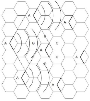
In sleep mode, BS energy consumption can be saved by switching off some cells as a function of the traffic loads. In this work, low traffic period is considered during 0a.m. to 9a.m. In this interval of time, sleep mode can be activated.

When sleep mode acts, 3 out of 4 cells can be switched off progressively when the number of the current UEs becomes less than a certain percentage of the maximum number of active UEs offered by the simulator (according to the condition of sleep mode activation listed in Table 5.4).

In this sleep mode scheme, 1 out of 4 cells remain permanently active in order to guarantee the minimum coverage as depicted in Figure 5.1.

After 9a.m., cells switch on progressively to turn the cellular network into normal mode.

During the simulation, the server updates the sleep mode status at every multiple of the server granularity.

Then, in the sleep mode updating process, the server firstly verifies the number of active UEs in each activated cell, and then it decides whether some cells could be switched on.

According to Scenario 1 of Figure 3.2, active cells may zoom out to compensate the coverage holes by increasing the transmit power and/or the cell radius (i.e. adjusting the tilt of the antennas and by pointing them to a more distance border where it has the greater gain).

However in Scenario 2 of Figure 3.2, there are no increases in the transmit power and/or the cell radius.

We denominate these models of sleep mode as: “Sleep mode (increase of the transmission power/cell radius increase ratio)_”.

Some examples of sleep mode denominations are listed in Table 5.3

Table 5.3 - Examples of sleep mode denomination

Sleep mode

denomination transmit power Increase of the increase ratio Cell radius Observations

Sleep mode (+0dB/1x) +0dB 1x Does not increase the transmit _{power and the cell radius}

Sleep mode (+0dB/2x) +0dB 2x Doubles only the cell radius

Sleep mode (+3dB/1x) +3dB 1x Increases only the transmit _{power of 3dB}

Sleep mode (+3dB/2x) +3dB 2x Increases the transmit power of 3dB and doubles the cell radius