Interpolation methods for creating a scatter radiation exposure map

OF

RADIATION SCIENCES

BJRS

Interpolation methods for creating a scatter radiation

exposure map

Elicardo Alves de Souza Goncalves¹, Celio Simonacci Gomes², Luis Fernando

Oli-veira³, Marcelino Jose Anjos³, Davi Ferreira OliOli-veira³, Ricardo Tadeu Lopes²

Janeiro

[email protected]

ABSTRACT

A well known way to understand radiation scattering and radiation exposure ratings, in a procedure that makes use of ionizing radiation, is to map its exposure over the space around the source and the sample. This map is done by measur-ing exposure in points regularly spaced, that is, measurement will be done in places defined by regular steps, startmeasur-ing at a point and moving along the x, y and z axes or, in a more efficient way, using radial and angular coordinates. However, it is not always possible to maintain the steps’ accuracy throughout the entire space, or there would be regions of diffi-cult access where the steps’ regularity would be compromised. In this work, we use a high energy radiation source to simulate a common radiography setup and construct its exposure map. The points’ arrangement and the interpolation were used considering polar coordinates. Then, with the same data, an interpolation using the Delaunay triangulation was made. The results show the advantages and disadvantages of each one, in addition to providing a high coherence to the data. To simulate the impossibility of regular points, the same procedures were performed in the absence of any point and compared. The results show a lower total variation when the map is calculated by triangulation. The computa-tional and graphic treatment was performed with GNU OCTAVE software and its image processing package. The data were acquired from a bunker where a 6MeV betatron was used as a primary source.

Keywords: Radiation Scattering; Betatron; Radiation Exposure Control;

1. INTRODUCTION

In addition to the main beam, which is possible to accurately find and therefore is easier to avoid, scattered radiation is one of the concerns regarding radiation protection. Positioning, range, intensi-ty, and direction of the beam within the space involved with radiography may be important in de-creasing occupational and accidental doses. This becomes more important when the procedure is done outdoors, with a mobile radiation source, in a place with many scatter sources or with a high exposure rate [1].

Because of the isotropic characteristics of radiation, protection procedures are often only concerned about the exposure regarding distance to the sample, considering the radius the only variable. It is a good approach for regular, simple samples, with an unelevated energy beam and an easy incidence angle. In this situation, it´s possible to take a conservative practice and estimate doses always look-ing for the larger radius [1-3].

However, for many reasons, scattered radiation added to mean beam and leakage radiation won’t be totally isotropic, and it means that there could be directions in which exposure gradient is higher [2,3]. Because of this, in order to achieve a very accurate measurement, especially in cases of unu-sual angles and high energy levels, it´s possible to create a spatial exposure map, measuring a great number of points around the radiography setup [3-5]. Since the map is a continuous function, built using punctual information, interpolation is necessary to estimate values in order to fill in the spaces between the points.

At the first approach, one could thing about a Cartesian map with equal regular steps between points among the x, y and even z axis [6]. It´s reasonable since, in that way, each measure will be a pixel in a 2D map. But, if it´s reasonable to think the behavior of radiation coming in isotropic way from a punctual source, maybe it is better to think about angular coordinates [3,5].

Despite it is better than Cartesian, an image created from angular coordinates may present some problems due to the inequality of weight of each point, and the fact that the radius coordinate could

be more important than the angle coordinate. This problem can become more important if steps are not regularly spaced or missed [3-5]. Due to several reasons, many points could be missing or even not marked, letting a coordinate list incomplete for the map. It may cause imprecision, wrong esti-mates or even aliasing on the map [3].

This work intends (A) to create a map of a high energy source using angular coordinate method in a traditional way, describing in detail it’s confection process. Then, (B) to compare it, using the same dataset, to the Delaunay triangulation interpolation method. To show a situation where the Delaunay approach could be useful, the same maps were built with some points missing, in order to estimate how each method behaves when some information is absent. The data were acquired using a setup with a 6MeV betatron exposing a tubular steel sample in order to simulate a radiography procedure. The GNU OCTAVE software and its image processing package were used to process information and to build the visual information.

2. COORDINATE SYSTEMS

Because each image is a rectangular matrix of pixels, the easiest way to generate images is through Cartesian coordinates. The similarity between the pixel’s location and the x and y coordinates leads us to an image of a huge cartesian dataset, where each point is a pixel in the image. The interpola-tion is done to increase the amount of data, decreasing spaces between points. It is done using the values and distances from the neighbor points, with simple mathematical tools. To read points in a way to perform cartesian coordinates, the points must be regularly spaced, in two orthogonal direc-tions. The great advantages are the precision and the equal importance of the points; the disad-vantage is the large number of points to cover a certain area. It also takes a lot of non-important information, mainly about a relatively homogeneous medium, like the air around the source and the sample [3].

The ionizing radiation behavior throughout space is well described and known. A typical source emits radiation isotopically. Even when the emission is anisotropic, it could be well fitted in an iso-tropic mathematical function. The intensity on space is inversely proportional to the square of the

distance. It means that for polar coordinates (two dimension) and spherical coordinates (three di-mension) the radial information is more important than the angular one [3-5].

A sample, the medium or even the obstacles could be considered as a sum of several punctual sources, eventually with anisotropic emission. It means that, except for the case of a very specific geometry, distance will be the most important variable. In many situations, each direction has its own exposure rate, which also can be fit in the inverse square law. In a conservative way, it is pos-sible to take the direction with the highest exposure and consider its values in all directions creating rings of super estimated exposures.

All of these facts suggest polar (or spherical) coordinates to create an exposure map, as done in many works [2-7]. But there are many problems too. The main problem is about the weight of each point: it is different, and a mistake or an abrupt change in a single measure could change signifi-cantly a great part of the map. This is a direct consequence: due to the smaller number of points, some points will cover a bigger region.

Another problem is the conversion between this coordinate system and the image’s pixels map, once the pixel location is similar to a Cartesian system, and each pixel location has only values in whole numbers. It is necessary to use approximated decimal values in order to correlate each pixel. Points measured when thinking on polar coordinates are centered on the source or on the sample, varying the distance (radius) and direction (angle) from the center. To use these data and convert them into an image, there are two ways: the first is to build a map still based on polar coordinates, interpolating r and θ information and then convert each new point to a pixel on image. The second method consists of converting each measured point into a cartesian system and then interpolate it building an image map. This last way brings to the cartesian system of points positioned at a non-regular distance of one another, demanding on different mathematical tools to perform the interpo-lation.

The Delaunay method consists of creating a lot of little triangles in which the vertices are the col-lected data points. The exposure function depending on x and y is a surface in a three-dimensional space and these triangles make a good approach to this surface [8-9]. If the triangle in a specific lo-cation is known, it´s possible to estimate the value of exposure at that lolo-cation. Despite it is only a linear interpolation [8-9], it´s relatively efficient, produces good spatial resolution, and covers a greater area, forming a polygon around the sample.

3. MATERIALS AND METHODS

3.1 Acquired data

The data used in this work has been acquired on a bunker of 6 x 6 x 6 meters, where a 6 MeV betatron was exposing a 400 mm diameter steel tube. The tube was positioned at the center of the bunker, and the measured points were placed around it. In each point the accumulated exposure for 30 seconds was ready. Using the sample as the center of system, angular direction of 45º, 90º, 135º, 180º, 225º, 270º, 315º and 360º, and the radial distances of 500, 1500 and 2500 mm, the measures were taken, resulting in a dataset of 24 points. The markings to position measurements are shown in Image 1. An ionizing chamber Radical 10x6-6 and a Radical dose meter system 2186 was used to measure each point.

The interpolation to create the image was made in the two formerly described ways: creating a map in the r and θ space and then converting all the map to a pixel matrix; and converting the original points to a cartesian pixel map using the Delaunay triangulation to fill in the rest of the image.

3.2 Transformation after data interpolation: the conventional treatment

The data acquired on polar regular steps can be plotted in the radius versus angle domain. On the r and θ space, these variables could be treated like cartesian ones, as two orthogonal axes. It means that they could pass through the same process than the cartesian. After choosing the resulting matrix’s size (in number of pixels) the conversion was done. It is important to say the computer routine makes the image pixel by pixel, scanning the resulting image, not the resulting measured points. The bicubic interpolation was performed in r and θ space, instead of bilinear. It considers the fit of degree 3 polynomial functions in the directions x and y and could give the interpolation more precision. The process was made in a GNU OCTAVE and it is described on the follow steps:

• Start from the first pixel.

• Convert the column numbers and calculate the pixel into x and y coordinates of the Cartesian plan. • Convert the x and y coordinates into R and θ of polar coordinates.

• With the data acquired, perform a bicubic interpolation to estimate the exposure value at the R and θ coordinates.

• Take the estimated value of the pixel. • Repeat the process on the next pixel.

3.3 Delaunay triangulation method to scatter data interpolation

The data acquired on polar regular steps was directly transformed into Cartesian coordinates, and the interpolation was done on the xy domain. In this situation R and θ were values measured in whole numbers, but x and y were not. The direct conversion produced a lot of irregular coordinates on xy domain, and the simplest interpolation couldn´t be done. A GNU OCTAVE routine was built to perform triangulation interpolation. In this case, computer routine works scanning the measured data, not the pixel matrix. The entire conversion can be done on the following steps:

• Start from the values measured at the points.

• Convert the R and θ of polar coordinates into x and y coordinates of Cartesian system. • Find the triangles system based on Delaunay method.

• Fill the empty pixels (considering certain limits) performing 2d linear interpolation between triangle vertices.

• adjust and/or scale image.

3.4 Simulating lack of points

After creating the maps, data was submitted again to the two interpolation routines described before. At this time, without one point, in order to compare it to a map made using all the data. A standard deviation was calculated to compare it. Another GNU OCTAVE routine was created to do the following steps.

• Take the data set.

• Take the maps created by the entire data set. • Erase the first point of the data set.

• Perform the interpolation routine described before.

• Calculate the standard deviations between the new map and the original map for each method. • Save the standard deviation value in a cumulative variable (one for each interpolation method). • Take the data set again and perform the previous steps erasing the next point.

4. RESULTS

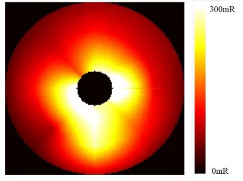
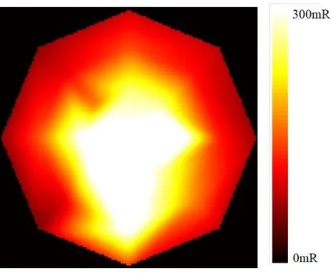
Table 1 shows the values obtained. The resulting Maps, from the conventional and triangulation interpolation, are displayed in Image 2 and 3. Image 4 represents how these maps fit in the bunker.

distance\direction 0º 45º 90º 135º 180º 225º 270º 315º

500mm 270 184 180 108 217 232 250 187

1500mm 83 79 98 69 100 63 225 117

2500mm 38 51 55 37 33 29 70 45

Figure 2: Map from data interpolated before transforming it to the Cartesian form. A round

non-mapped area on the center is due to measurement limitations.

Figure 3: Map created from interloping data using triangulation after coordinates transformation.

Figure 4: Map created inside the bunker set representation from each one of the interpolations: (A)

from conventional data treatment and (B) Delaunay interpolation.

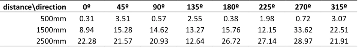
When a point lacks, the first method has a mean standard deviation around 12.9 mR and the second, about 8.3 mR. Tables 2 and 3 show the standard deviation for absence of each point for this calculation.

distance\direction 0º 45º 90º 135º 180º 225º 270º 315º

500mm 0.31 3.51 0.57 2.55 0.38 1.98 0.72 3.07

1500mm 8.94 15.28 14.62 13.27 15.76 12.15 33.62 22.51 2500mm 22.28 21.57 20.93 12.64 26.72 27.14 28.97 21.91

Table 3: Standard deviation due to the lack of each point in the Delaunay method. Values in mR.

distance\direction 0º 45º 90º 135º 180º 225º 270º 315º 500mm 0,01 13,17 16,44 10,99 14,89 15,71 23,80 17,00 1500mm 0,01 4,72 2,88 5,43 11,68 10,26 12,74 8,63 2500mm 11,50 4,58 5,75 8,78 10,61 7,44 7,16 7,75

It is possible to see that conventional interpolation didn´t create new data outside the measured re-gion. This way, the non-measured center where the sample is presents no information about expo-sure. Instead, this method estimates how the exposure could be if no abrupt change in behavior hap-pens on the center. Another interesting fact is about patterns. While the first method has strong dif-ferences between directions causing radial marks, the second one has triangular patterns, due to the mathematical method. The triangulation interpolation, on the other hand, fills the unmeasured cen-ter in the data. For this data with few points, the lack of one point shows, at least in a general view, that the second method results on less changes, depending on a single missing point.

5. DISCUSSION

In the first method used, measurements were taken in points concerning polar coordinates with the sample (which is probably the principal source of scattered radiation) at the center and this data was used to find values corresponding to the exact pixel location on a square matrix image. This is due to the fact that in R and θ domain both coordinates don´t have the same weight as coordinates, when it comes to image reconstruction. In fact, interpolation in R could be done with a different method than θ.

As all the interpolation occurs in R and θ domain, no data is estimated outside the range of R. Be-cause no measurements are also done inside the sample, the map presents a non-informed region in

the middle. Because the sample could be viewed as an obstacle, it is the only region where interpo-lation might not be the best way to estimate exposure distribution. The same occurs outside, when the data output is a circle generating a round map. The region near the outside edge of the circle, is probably the less accurate data, due to its great area depending on few points.

The second method, using the same measurements, first converts the data into Cartesian domain, which is the most likely pixel position in an image. As a result of this, points aren´t regularly spaced on x and y coordinates as in a crossed on a grid. So, the interpolation method is needed to take non-regularly spaced matrix and estimate the regular points. The method used is the Delaunay triangula-tion (well known in image rendering process), where each point of the data (with its three coordi-nates: x, y and value measured) is considered as a vertex of a triangle. In a good approach, triangles form an almost equal surface than data on a 3D plot. A point outside the data can be found using the planned equation of each triangle. This causes a specific bilinear interpolation which depends pri-marily on the three points at the triangle vertices. It can be said that this is the reason for less varia-tion on the standard variavaria-tion, but that’s not entirely true, because once a point is suppressed on this process, a completely different triangulation could be done.

There are many consequences in triangulation usage. The most easily noted is a triangle pattern in the final image. Because these data are acquired in eight different directions, the area mapped due to interpolation is an 8 faced polygon. The edges are very dependent from extreme point and probably have the higher statistical fluctuation.

Of course, the number of points and their distribution are important, in a way that even many points equally covering all the map mean less errors. In a dynamic way, it is possible to suggest that re-gions with higher gradient will have more points. It means that to minimize the number of points without losing accuracy of measurement, a software could indicate where the next point may be measured. It will make the maps’ production method faster and more efficient.

6. CONCLUSION

Interpolation estimates non-existing data from existing ones, and in some cases, it can be a good approach to improve spatial resolution, even with fewer data points. Homogeneous spaces like a

room filled with air is a good example of where it could work well, because the lack of obstacles results in an exposure distribution with no abrupt change.

With the same data, different interpolation types create similar maps, but not equal ones. The tradi-tional approach, using polar coordinates, makes a circular map with smooth variations, mainly on radius direction. The alternative approach, using the not gridded data as cartesian coordinates and performing Delaunay triangulation causes a triangular pattern, making a map which is similar to the previous one.

Another interesting fact in resulting image is the filled center, even without measurement. This is a direct consequence of using interpolation in the x and y domain, because for the interpolation pro-cess it is like empty values inside the interest region. Despite our decision of not removing it from the image, it´s not safe to imply that the values are correct, because the sample works like an obsta-cle and, inside it, changes could be more abrupt, so it isn’t like the air medium. Besides, our models aren´t about primary radiation, which can´t be forgot when talking about radiation on the sample.

Standard deviation demonstrates the difference between losing a single point in each method. Be-cause of its nature, but also due to its interpolation mathematics, the first method changes more, and it makes a standard deviation until 50% larger. It is believed that the mean of this standard deviation shows any stability of result, changing or losing data, but this is a panoramic information and for specific cases, more accurate details will be necessary.

REFERENCES

1. IAEA - International Atomic Energy Agency. Radiation protection and safety in industrial

radiography. Viena: IAEA- Safety report series, 1999. 69p

2. CHIANG, H. W.; LIU, Y. L.; CHEN, T.R. CHEN, C. L.; CHIANG, H. J.; CHAO, S.Y. Scattered radiation doses absorbed by technicians at different distances from X-ray exposure: Experiments on prosthesis. Bio-medical materials and engineering. V.26, p.S1641-S1650, 2015.

3. REHN, E. Modeling of scatter radiation during interventional X-ray procedure, Master thesis, Linkoping University, Linkoping, Sweden, 2015. 46p.

4. KUON, E.; DAHM, J.; EMPEN, K.; ROBINSON, D. M.; REUTER, G; WUCHERER, M. Iden-tification of less-irradiating Tube angulations in invasive cardiology. Journal of the American

College of Cardiology. v44, n.7, p.1420-8, 2004.

5. HAQQANI, O. P.; AGARWAL, P. K.; HALIN, N. M.; IAFRATI, M. D. Defining the Scatter cloud in the interventional suite. Journal of vascular surgery, v.58, n.5, p.1339-45, 2013.

6. ALONSO, J. A.; SHAW, D. S.; MAXWELL, A.; McGill, G. P.; Hart, G. P. Scattered radiation during fixation of hip fractures. Is Distance alone enough protection? Journal of Bone and Joint

Surgery, v.28-B, n. 6, p.815-8, 2001.

7. ALDEWAINI, Z.; LANGER, E.; SCHABER, P.; DAVID, M.; KRETZ. D.; STEIL, V.; HESSER, J. Real-time, ray casting-based scatter dose estimation for c-arm x-ray system, Journal

of Applied Clinical Medical Physics, v.18, p.144-53, 2017.

8. ASTRAHAN, M. A.; STREETER, O. E.; JOZSEF, G. Calculation of mean central dose in inter-stitial brachytherapy using Delaunay triangulation, Medical Physics, v.28, n.6, p.1016-23, 2001. 9. JOZSEF, G.; STREETER, O. E.; ASTRAHAN, M. A. The use of linear programming in optimi-zation of HDR implant dose distributions, Medical Physics, v.30, n.5, p.751-60, 2003.