Design of a Low Consumption Electric Car Prototype

(1)

UNIVERSIDADE DA BEIRA INTERIOR

Engenharia

Design of a Low Consumption Electric Car

Prototype

Carlos Magno dos Reis Fonte

Dissertação para obtenção do Grau de Mestre em

Engenharia Aeronáutica

(Ciclo de estudos integrado)

Orientador: Prof. Doutor Miguel Ângelo Rodrigues Silvestre

(2)

(3)

iii “The phenomenon of turbulence was probably invented by the Devil on the seventh day of Creation (when the Good Lord wasn't looking)” Peter Bradshaw

(4)

(5)

v

Dedicatória

Dedico esta dissertação de mestrado aos meus pais, Carlos Gonçalo Silva da Fonte e Elisabete do Céu Pires dos Reis Fonte e também à minha namorada Hilary Almeida Marques, por todo o apoio dado ao longo destes anos e por terem acreditado nas minhas capacidades. Esta dissertação é para vocês!

(6)

(7)

vii

Agradecimentos

Quero agradecer o Professor Doutor Miguel Ângelo Rodrigues Silvestre, orientador desta dissertação, ao Professor Doutor José Carlos Páscoa Marques e ao Doutor Carlos Xisto a partilha do conhecimento e da ajuda valiosa para este projeto.

Também quero agradecer a todos os meus amigos, família e minha namorada pelo grande apoio dado e tempo dedicado. Muito Obrigado!

(8)

(9)

ix

Resumo

Preocupados com o ambiente e a sustentabilidade, a Shell organizou nos últimos 30 anos uma competição de veículos de baixo consumo designada por Shell Eco-Marathon (SEM). O objetivo do veículo é atingir a velocidade média mínima de 25 / , sendo o valor reduzido de arrasto um parâmetro importante para atingir um bom resultado. Ao longo dos anos as equipas da SEM usaram corpos fuselados parecidos com perfis alares e com uma baixa área frontal, contudo a presente equipa AERO@UBI decidiu criar um novo conceito para o desenho da carroçaria do veículo. Este corpo 3D também deriva de um perfil alar, usando uma transformação geométrica proposta por Galvão em 1968 em "Nota técnica sobre corpos fuselados", São José dos Campos, para a criação de corpos fuselados. De acordo com esse autor, é possível replicar a distribuição do coeficiente de pressão do perfil alar para o corpo 3D. Deste modo, mantêm-se as características de baixo arrasto do perfil alar. Através do uso do software CFD ANSYS Fluent fomos capazes de confirmar o conceito usado e examinar a aerodinâmica do veículo. Apesar do resultado não ter sido o ótimo, foi possível confirmar a teoria introduzida por Galvão. O veículo tem um comportamento similar ao do perfil com um 0.088 para uma área frontal de 0.3522 . A análise dos resultados mostram que algumas modificações são necessárias para otimizar o veículo. Uma possível modificação é ajustar a transformação do perfil alar a fim de reduzir a acuidade do nariz para um melhor acordo entre o corpo 3D e a distribuição do coeficiente de pressão do perfil alar. Todavia, é possível com este conceito obter corpos de arrasto reduzido com uma transição da camada limite tardia, o que significa um consumo menor, tanto para aeronaves quanto para veículos terrestres.

Palavras-chave

(10)

(11)

xi

Resumo Alargado

Preocupados com o ambiente e a sustentabilidade, a Shell organizou nos últimos 30 anos uma competição de veículos de baixo consumo designada por Shell Eco-Marathon (SEM). O objetivo do veículo é atingir a velocidade média mínima de 25 / , sendo o valor reduzido de arrasto um parâmetro importante para atingir um bom resultado. Ao longo dos anos as equipas da SEM usaram corpos fuselados parecidos com perfis alares e com uma baixa área frontal, contudo a presente equipa AERO@UBI decidiu criar um novo conceito para o desenho da carroçaria do veículo. Este corpo 3D também deriva de um perfil alar, usando uma transformação geométrica proposta por Galvão em 1968 em "Nota técnica sobre corpos fuselados", São José dos Campos, para a criação de corpos fuselados. De acordo com esse autor, é possível replicar a distribuição do coeficiente de pressão do perfil alar para o corpo 3D. Deste modo, mantêm-se as características de baixo arrasto do perfil alar. O corpo 3D diz respeito a um corpo de revolução do perfil alar transformado. A partir desse corpo de revolução é aplicado o conceito de áreas equivalentes, sendo assim possível alterar as formas das secções transversais do corpo de revolução para uma melhor adaptação aos sistemas internos do veículo mantendo as características aerodinâmicas do perfil alar. O uso de um perfil alar conveniente é importante para este projeto, por isso foram impostos alguns critérios para a escolha do perfil, como uma grande extensão laminar e um baixo valor de arrasto. Através do uso do software CFD ANSYS Fluent fomos capazes de confirmar o conceito usado e examinar a aerodinâmica do veículo. Apesar do resultado não ter sido o ótimo, foi possível confirmar a teoria introduzida por Galvão. O veículo tem um comportamento similar ao do perfil com um 0.088 para uma área frontal de 0.3522 . A análise dos resultados mostram que algumas modificações são necessárias para otimizar o veículo. Uma possível modificação é ajustar a transformação do perfil alar a fim de reduzir a acuidade do nariz para um melhor acordo entre o corpo 3D e a distribuição do coeficiente de pressão do perfil alar. Todavia, é possível com este conceito obter corpos de arrasto reduzido com uma transição da camada limite tardia, o que significa um consumo menor, tanto para aeronaves quanto para veículos terrestres.

(12)

(13)

xiii

Abstract

Concerned with environment and sustainability, Shell has organized for the last 30 years a competition of energy efficient road vehicles called Shell Eco-Marathon (SEM). The vehicle is required to achieve a minimum mean cruise speed of 25 / and a low drag value is an essential parameter to achieve a good result. Over the years SEM teams used a streamlined body similar to an airfoil with a minimized low frontal area, however AERO@UBI team decided to create a new concept vehicle body. This 3D body also derives from a 2D airfoil, but a geometric transformation introduced by Galvão in 1968 in "Nota técnica sobre corpos fuselados", São José dos Campos, for the creation of low drag fuselage is used. According to that author, it is possible to replicate the pressure coefficient distribution of the airfoil in the 3D body. Thus, maintaining the airfoil's low drag characteristics. Through the use of CFD software ANSYS Fluent it was possible to confirm the used concept and examine the vehicle aerodynamic. Although the final result was not optimal, it was possible to confirm the theory introduced by Galvão. The vehicle does have the same behavior as the airfoil with a 0.088 for a frontal area of 0.3522 . The results show that some modifications need to be made a future works to optimize the vehicle. One possible modification would be to adjust the airfoil transformation in order to decrease the sharpness of the vehicle’s nose for a closer agreement between the 3D body and the airfoil's pressure coefficient distribution. Nevertheless, with this concept it is possible to design low drag bodies with late boundary layer transition which means a lower drag and energy consumption, both for airplanes and road vehicles.

Keywords

(14)

(15)

xv

List of Figures

Figure 1.1 - AERO@UBI vehicle at Eco-Shell Marathon Europe 2015 edition ... 1

Figure 1.2 - Maubere from UBI team ... 2

Figure 1.3 - UBIcar 2012 from UBI team ... 3

Figure 2.1 - 3D axis system to define aerodynamics forces ... 5

Figure 2.2 - Lift and drag coefficient variation with ground clearance [5] ... 6

Figure 2.3 - Minimal ground clearance [6] ... 7

Figure 2.4 - Representation of angle of attack for an airfoil ... 7

Figure 2.5 - Lift and drag coefficient versus angle of attack for a generic sedan [7] ... 8

Figure 2.6 - Illustration of forces produced by the fluid. a) Tangential force. b) Perpendicular force. c) Mixed forces. ... 8

Figure 2.7 - Representation of a) Frontal area and b) Wet area ... 9

Figure 2.8 - Basics conceptual shapes (Adapted from [7]) ... 10

Figure 2.9 - Blockage effect illustration a) Wide away walls b) too-close walls [7] ... 13

Figure 2.10 - Sketch of boundary layer on a flat plate in parallel flow at zero incidence [14] 14 Figure 2.11 – Near wall region turbulent flow subdivision (Adapted from [15]) ... 15

Figure 2.12 - Dimensions of Ahmed Body ... 16

Figure 2.13 - Pac Car II from ETH Zurich team [20] ... 17

Figure 2.14 - ARTEMIDe from XTEAM [21] ... 18

Figure 2.15 - IDRApegasus from H2politO team [24] ... 18

Figure 2.16 - Microjoule from La Joliverie team ... 19

Figure 2.17 - Fancy Carol from Japan ... 19

Figure 3.1 - NACA 0012 transformation by equation (3.1) ... 22

Figure 3.2 - Flowchart of implemented concept ... 23

Figure 3.3 – 3 Views of pilot position a) Front view b) Side View c) Top View ... 24

Figure 3.4 - 3D view of first design of the vehicle configuration concept ... 24

Figure 3.5 - 3 Views of first design of the vehicle configuration concept. Dimensions in [mm] a) Front View b) Side View c) Top View ... 25

Figure 3.6 - Example of transversal section ... 25

Figure 3.7 – Equivalent body of revolution of the initial design... 26

Figure 3.8 – Airfoil created on XFLR5 for the vehicle design ... 28

Figure 3.9 - Variation of Drag coefficient with angle of attack Re=1500000 ... 29

Figure 3.10 - Longitudinal position of the boundary layer transition Re=1500000 ... 29

Figure 3.11 - Coordinate distribution ... 30

Figure 3.12 - Lateral view of asymmetric body created for support design ... 31

Figure 3.13 - Multiple section sketch of AERO@UBI ... 31

Figure 3.14 - Vehicle shape after some sculpt modifications on Blender ... 31

(18)

xviii

Figure 3.16 - Final coordinate distribution of the vehicle ... 32

Figure 3.17 - Structured mesh representation - , ⇐ data stored on a 2D array ... 33

Figure 3.18 - Dimensions for control volume (half body) and boundary mesh labels ... 34

Figure 3.19 - Bounding box definition ... 34

Figure 3.20 - Position of the vehicle body on the control volume bounding box ... 35

Figure 3.21 - Surface refinement level definition for the body ... 36

Figure 3.22 - a) Level 1 of surface refinement b) Level 2 of surface refinement ... 37

Figure 3.23 - Pointwise online Y+ calculator ... 37

Figure 3.24 - Layer definition ... 37

Figure 3.25 - Detailed view of created layers on the body surface ... 38

Figure 3.26 - Detailed view of missing and deformed layer zones ... 38

Figure 3.27 - Definition of cell refinement from a given distance ... 39

Figure 3.28 - Geometrics figures for zone refinement ... 39

Figure 3.29 –Detailed view of mesh result from HELYX-OS ... 39

Figure 3.30 - Log file from HELYX-OS ... 40

Figure 3.31 - Wall y+ distribution in the half vehicle surface ... 41

Figure 3.32 - Comparison of Pressure-Based Segregated Algorithm and Pressure-Based Coupled Algorithm [10] ... 43

Figure 3.33 - Result comparison for Ahmed Body ... 44

Figure 4.1 – Transformed airfoil body of revolution ... 45

Figure 4.2 - Drag coefficient (on h times b) of transverse gaps [3]. ... 46

Figure 4.3 - Drag coefficient based on area b times d of wheels ... 47

Figure 4.4 - Average Pressure Coefficient distribution ... 49

Figure 4.5 - Average Pressure Coefficient distribution for different ground clearance of AERO@UBI ... 49

Figure 4.6 - Wall shear stress in x-direction of AERO@UBI showing small regions of separated flow in the final vehicle body design ... 50

Figure 4.7 - Wall shear stress in x-direction of axisymmetric body showing small regions of separated flow in the vehicle body equivalent body of revolution ... 51

Figure 4.8 - Wall shear stress in x-direction of axisymmetric body with ground symmetry boundary ... 51

Figure 4.9 - Drag coefficient and Downforce coefficient variation with ground clearance ... 53

Figure 4.10 - Definition of negative angles direction. ... 54

Figure 4.11 - Drag coefficient and Downforce coefficient variation with angle of attack ... 54

Figure 4.12 - Average coefficient pressure distribution for different exponential values ... 55

(19)

xix

List of Tables

Table 3.1 - Data for the calculation of the vehicles body Reynolds number ... 27

Table 3.2 - Typical values of NCrit for various situations [37] ... 28

Table 3.3 - Boundary Conditions ... 41

Table 3.4 - Reference Values ... 42

Table 3.5 - Pseudo Transient Explicit Relaxation Factors ... 43

Table 4.1 - Vehicle comparison results ... 45

Table 4.2 - Definition of cavities dimensions ... 47

Table 4.3 - Definition of wheels dimensions ... 48

Table 4.4 - SEM vehicles comparison ... 48

Table 4.5 - CFD results for different boundary conditions for the ground ... 52

Table 4.6 - Ground Clearance influence results ... 52

Table 4.7 - Angle of Attack influence results ... 53

(20)

(21)

xxi

List of Abbreviations

SEM – Shell Eco-marathon CFD – Computer Fluid Dynamics DNS – Direct Numerical Simulations LES – Large Eddy Simulation

RANS – Reynolds-Averaged Navier-Stokes STL - Surface Tesselation Language GUI - Graphical User Interface

(22)

(23)

xxiii

List of Symbols

- Fluid density ⁄ – Fluid velocity ⁄

– Wetted area (surface area) – Frontal area

– Frontal area of the component – Frontal area of the vehicle

– Drag coefficient – Lift coefficient

, – Skin friction drag coefficient , – Pressure drag coefficient

⁄ – Dimensionless horizontal position of the airfoil

– Dimensionless horizontal position of the revolution body – Dimensionless radius of the revolution body at position

– Dimensionless vertical coordinate of the airfoil at position ⁄ – Section radius

– Transversal area of the section – Reynolds number

- Vehicle velocity ⁄ – Vehicle length

– Dynamic viscosity ∙ ⁄ – Distance from the wall – Fluid density

- Viscosity

- Non-dimensional wall unit - Non-dimensional velocity unit – Wall shear stress

, and – maximum distance from the references plans for each axis , and – minimum distance from the references plans for each axis , and – number of elements for each axis

– Surface Cell Size

– Bounding Box Cell Size – Refinement Level

– Relative Final Layer Thickness ∆ – Expansion Rate

– Number of Layers ∆ ∗_{- First cell height}

(24)

(25)

1

Chapter 1

1. Introduction

1.1 Introduction

The purpose of the present work was to design a vehicle body for a Shell Eco-Marathon (SEM) vehicle and study it through CFD simulation in order to evaluate its performance and possible improvements to the design concept.

The AERO@UBI is a battery electric prototype vehicle (Error! Reference source not found.) build by a team from Aeronautical Engineering of University of Beira Interior (UBI). AERO@UBI participated in the electric prototype category in SEM Europe 2014 and 2015 editions. On 2014 edition due to a technical issue in the motor controller it was impossible to achieve any results in the circuit. But, in 2015 with the controller problem fixed a 19th_{place was achieved with a}

consumption of 330.8 ⁄ .

Figure 1.1 - AERO@UBI vehicle at Eco-Shell Marathon Europe 2015 edition

Since the drag force value is an important parameter, it must be minimized to achieve a good result in SEM. With this in mind, a new concept of vehicle design was implemented herein for research.

In 1968, Aeronautical Engineer Francisco Leme Galvão introduced a concept where he explains that from a geometrical transformation of a 2D airfoil we can maintain similar aerodynamics

(26)

2

characteristics in a 3D body [1]. This concept was used to generate the present vehicle’s body design. To evaluate it, Reynolds Averaged Navier Stokes (RANS) with turbulence model closure Computational Fluid Dynamics (CFD) simulations were performed with ANSYS Fluent software.

1.2 Shell Eco-Marathon Background

SEM is a racing competition dating back to 1939 when Shell Oil Company employees in USA made a bet over who could travel more kilometers with the same amount of fuel. In 1985, Shell revived the event starting the SEM annual competition. Since then, the competition expanded to two more continents, Europe and Asia. The teams compete in one of two possible categories: prototype and urban concept. These categories are split by energy type, internal combustion with various fuels, electric or hybrid propulsion. The prototype category has the objective of minimizing energy consumption despising the pilot comfort. The urban concept category focuses on practical designs. Regarding the energy type, internal combustion engine fuel types include: petrol; diesel; liquid fuel made from natural gas; ethanol and compressed natural gas, and electric propulsion can be powered by hydrogen fuel cells or lithium-based batteries. Every year hundreds of teams show their vehicle concepts and test them on the track to achieve the highest range on the equivalent of one liter of fuel or one energy measuring unit, in the case of the present battery electric vehicle. A good streamlined vehicle is important to decrease the drag force value, which is a critical parameter on prototype’s concept, and thus achieve a good result. However the vehicle is constrain by some rules, from dimensions to safety, not impeding the creation of very low drag vehicles. One of the best examples of a prototype vehicle is the Pac Car II from ETH Zurich team (see Figure 2.13) beating the world record with a consumption of 5385 ⁄ .

In 1999 the first team from UBI participated in SEM competition with the Maubere (Figure 1.2). In the year 2000 edition, a consumption of 371 / was recorded. Twelve years later, in 2012, the same team but with an Urban Concept category vehicle won the first edition of a SEM similar competition, the Madrid Ecocity with 88 / (Figure 1.3).

(27)

3 For a prototype vehicle, since we have to decrease the drag force value, the solution found by most teams is to keep the frontal area in its minimum and create a streamlined body to prevent the flow separation such that the drag coefficient is kept as low as possible. Another design concept is to design the body with a curvature on the top in order to maintain the lift force value near zero. In the case of exterior wheels, the use of fairings can reduce the drag value but one has to be careful on fairings design because the wrong design can be prejudicial for the vehicle performance [2].

Figure 1.3 - UBIcar 2012 from UBI team

1.3 Objectives

The main objective of this project is to create a low drag vehicle for the AERO@UBI team SEM prototype vehicle while introducing a new concept of body shape creation and get all the information possible through RANS CFD simulation about the aerodynamics of the vehicle. It is also intended to verify the concept used for the first time in the creation of a road vehicle body, thus, introducing a new method of shape creation for low-drag vehicle bodies. To achieve this, the steps that have been followed during research were:

 The creation of the car body geometry and sizing with the intended new method;  Analysis of the air flow around the vehicle, monitoring the aerodynamics performance

parameters like drag, downforce and longitudinal pressure coefficient distribution;  Compare the vehicle body performance with an initial equivalent body of revolution

and the primitive airfoil;

(28)

4

 Analysis of the effects that angle of attack variation has on the vehicle;

 Based on the result of the different analyses, different variations of the vehicle shape are proposed for improvements.

1.4 Dissertation Structure

Following this introduction to the research topic, the next chapter presents a literature review covering the basic theory of road vehicle body design and adequate RANS CFD simulations and reports the state-of-art of SEM prototype vehicle body designs.

After the literature review, a chapter with an explanation of the methodology used throughout the study is given. The design concept and the drawing in CATIAV5 of the vehicle are explained in the first part. In the second part, the use of HELYX-OS for the mesh creation and the simulation settings of ANSYS Fluent software are described.

With the methodology explained, the results from the different simulations are presented and analyzed. From the analysis of the results, recommendations of improvements that could be implemented on the vehicle are presented.

Finally, a summary of conclusions and future works recommendations are listed in the last chapter.

1.5 Limitations and Dependencies

The main limitation of the present work was the available computational power. The mesh and simulations have been run on a laptop with a 2.5 CPU formed by two cores with 8 of RAM memory. Because of this limitation the mesh generation needed at last two days of iterations to create a mesh with an adequate quality and resolution. This limitation forced the mesh to have a poorer resolution than optimal, and the flow and vehicle geometry had to be simplified in order to reduce the mesh complexity and the cell number. A symmetry flow condition had to be applied to the vehicle symmetry plane, thus preventing the study of the flow sideslip angle on the body geometry design. The model is missing the wheels and respective cavities. This simplification changes the flow over the vehicle and the result of the simulations comparing to the actual vehicle flow. The drag generated by the real vehicle is, therefore, expected to be somewhat higher than the present results from the CFD simulations, but a prevision of the actual vehicle’s drag is given based on a correction for the missing items according to the book Fluid-dynamic Drag by Sighard Hoerner [3].

Although, a significant loss of time was initially caused by attempts of creating meshes with successive better quality for the body geometry, at the end, all presented results have passed the necessary mesh refinement tests, therefore satisfying the aims of the project.

(29)

5

Chapter 2

2. Literature Review

In this Chapter the basic theory behind the design of the present vehicle is explained. The chapter is split into three sections. The first thus covering the basics of road vehicle aerodynamics and the different parameters that affect the vehicle performance. Second, CFD simulation is covered and finally state-of-art of SEM vehicles is reviewed.

As we can see in Figure 2.1, the aerodynamic force can be considered as three distinct forces. These force are separated by 90 degrees, creating a Cartesian coordinate system. On the Z axis we have the vertical force named lift, on the X axis we have the horizontal force named drag, and on the Y axis we have the lateral force named side force. In our case we will focus on the lift and drag forces only.

Figure 2.1 - 3D axis system to define aerodynamics forces

In this road vehicle design context, in general, the vertical force will affect the vehicle on the opposite way of lift, which is, pushing the car towards the ground. Hence the value of the lift force will be negative. The correct term used to describe this force is downforce, which is the positive force towards the ground.

2.1 Basic Vehicle Body Design Parameters

The basics of the aerodynamics of a road vehicle are described on multiple theory books. For our case we will describe three important parameters that have a big impact on the vehicle’s aerodynamic performance. These are the ground clearance, the angle of attack of the body and its frontal area. All of these parameters depend mostly on the vehicle body shape.

(30)

6

2.1.1 Ground Clearance

Ground clearance can be described by the shortest distance between the flat road and vehicle body. In aerodynamics the ground clearance is one of the parameters affecting for the ground effect and so the downforce magnitude and the vehicle drag.

As we can see in Figure 2.2, downforce increases if ground clearance is reduced. That can be explained by the Bernoulli’s equation [4]. If the cross-section area of the gap between the body and the ground is reduced, the speed of the air flow must increase, thus generating a lower static pressure. The decrease of pressure will produce a suction effect directed to the ground, thus generating more downforce. This effect is called ground effect.

It’s also possible to see that a region exists where the ground clearance drops below h/L = 0.025. Here, the value of downforce decreases abruptly. This happens because at this non-dimensional distance the effects of viscosity start to be dominant, thereby “blocking” the flow under the body.

Figure 2.2 - Lift and drag coefficient variation with ground clearance [5]

Tamai explains in [6] that the drag of a moving vehicle as the same behavior as the Figure 2.3, where it is possible to see an optimal value of ground clearance regarding the minimization of drag. Tamai also suggest to set the minimal ground clearance between 0.15 and 0.25 for torpedo-shaped bodies.

(31)

7

Figure 2.3 - Minimal ground clearance [6]

2.1.2 Body Angle of Attack

The angle of attack is defined by the angle between the freestream (parallel to flight path) and the mean cord of an airfoil (see Figure 2.4). In aerodynamics the lift changes with the angle of attack and, generally, the greater the angle of attack, the greater the lift. For an airfoil if we have an excessive angle of attack, the flow separates the upper surface with a loss of lift that is denominated stall [4].

Figure 2.4 - Representation of angle of attack for an airfoil

The angle of attack of the body has a strong aerodynamic influence also in road vehicles like Katz [7] explains. In this case, the angle of attack is defined as the angle between the road and the vehicle’s x axis. The change of attitude on a vehicle is similar to a wing, that is, the lift increase when the angle of attack increases as it can be seen on Figure 2.5. For a smooth underbody vehicle the lift slope can be very large. The drag coefficient has a minor change when the angle of attack is changed, mainly due to a variation in the boundary layer thickness. In can be that the body incidence is an important parameter to take into account when designing the present SEM vehicle body. The shape of SEM vehicles in prototype category is typically very similar to a free falling drop, that’s why it’s important to consider the angle of attack to avoid an excessive value of downforce since the later would add normal force to the wheels rolling friction force.

(32)

8

Figure 2.5 - Lift and drag coefficient versus angle of attack for a generic sedan [7]

2.1.3 Frontal Body Area and Wetted Area

On a body moving through fluid, two distinct forces will be present throughout, one tangent to surface, (wall shear stress) and one perpendicular to the surface, (pressure) as it can be seen in Figure 2.6.

Figure 2.6 - Illustration of forces produced by the fluid. a) Tangential force. b) Perpendicular force. c) Mixed forces.

The integral of the tangential force on the body surface is called skin friction drag, , and the perpendicular force is called pressure drag, . The combination of this two type of drag form the total parasite drag, and they can be defined by:

1

2 , (2.1)

1

(33)

9 where:

- Fluid density ⁄ – Fluid velocity ⁄

– Wetted area (surface area)

– Frontal area

, – Mean skin friction coefficient , – Pressure drop drag coefficient

Analyzing the both equation it can be seen that the major factor to the variation of drag is the area. When the area increases, the drag increases also. Although these two drag react with different type of area definitions:

 Frictional drag depend on wetted area, area in contact with fluid flow, (see Figure 2.7b).

 Pressure drag depends mostly on frontal area1_{, area projected on a plane normal to the}

flow (see Figure 2.7a).

Figure 2.7 - Representation of a) Frontal area and b) Wet area

One can conclude that if we want to minimize the frictional drag we have to decrease wet area, on the other hand, if we want to minimize the pressure drag we have to decrease the frontal area. If no significant separation occurs, the frictional drag prevails, thus the main interest should be to minimize the wetted area.

2.1.4 Basic Aerodynamic Shapes

Basic shapes for vehicles that can create downforce with a minimum drag force are presented herein. Some of the possible shapes are shown in Figure 2.8.

(34)

10

The first shape configuration, Figure 2.8A, is aimed to reach a very low drag value, and is usually applied to speed-record vehicles that run along straightaways. With that configuration it is possible to change the value of downforce by adjusting the incidence/angle of attack of the vehicle. For high-speed turning vehicles, the best configuration is the inverted wing, Figure 2.8B, because of the ground effect produced by the wing and the low value of drag.

The “catamaran” concept, Figure 2.8C, is the shape usually used in prototype race vehicles. With the wheels covered by the two sides of the vehicle, it results in a shape with a central tunnel ending with a rear slope, making the under vehicle a venturi tube. Since the free stream is ducted under the vehicle, the area of flow separation is reduced on the back of the vehicle, creating an ideal high-downforce and low-drag configuration.

SEM vehicles use a concept similar to “catamaran”, but instead of the vehicle be covered on the two sides, only the wheels are covered, with the use of fairings. Reducing the effect of downforce and have a low-drag body.

Figure 2.8 - Basics conceptual shapes (Adapted from [7])

2.2 CFD Simulations of Road Vehicle Aerodynamics

Computational Fluid Dynamics (CFD) simulations are based on solving the equations of conservation that model fluid flows. One of the advantages of CFD simulations is that it is more affordable than an experiment in a wind tunnel. It is possible to realize a parametric study with a substantial reduction of lead time, study complex system under hazardous conditions with a great level of detail of results and work in large volume system impossible to conduct in an experiment [8].

(35)

11 CFD codes are structured around numerical algorithms that can tackle fluid flow problems. This structure is divided in three main elements, which are, a pre-processor, a solver and a post-processor [8].

2.2.1 Pre-processing

Pre-processing consists of the input of a flow problem to a CFD program and it can be divided in the following stages:

 Definition of the geometry of the region of interest - domain;

 Grid generation, which is, the division of the domain in small elements;  Selection of the physical phenomena that need to be modelled;

 Definition of fluid properties;

 Specification of appropriate boundary conditions.

The accuracy of a CFD solution is proportional to the number of elements (cells) in the grid, and generally for a larger number of cells the better is the solution. However it is important to see the relation between the accuracy of a solution and its cost in terms of necessary computer hardware and calculation time. For that reason it’s necessary to study the mesh independency of the solution to reach an optimal mesh with enough accuracy and minimal computational resources.

Is also important to select a good model depending on the physical phenomena. In the case of turbulence modelling we want to have a good and complete description of the turbulent flow, however an analytical solution doesn't exist even for the simplest turbulent flow. As it is known a turbulent flow is known as a function of space and time, and it can only be obtained by solving the Navier-Stokes equations [9].

To solve the problem of turbulence simulation some solutions exist, like Direct Numerical Simulations (DNS), Reynolds-Averaged Navier-Stokes (RANS) and Large Eddy2_{Simulation (LES).}

Direct Numerical Simulations (DNS) - The DNS is the most accurate simulation, since all the spatial and temporal scales of the flow are resolved by the time-dependent Navier-Stokes equations without any simplifying assumption.

Large Eddy Simulation (LES) - The turbulent flow is characterized by eddies with a wide range of length and time scales where:

2_{Eddy – Is the swirling of a fluid when the fluid flows past an obstacle, thus creating a reverse}

(36)

12

 The largest eddies are compared to the characteristic length of the mean flow;  The smallest scale are responsible for the dissipation of turbulence kinetic energy. Reynolds-Averaged Navier-Stokes (RANS) – RANS simulation is a simplest version of DNS, where the Navier-Stokes equations are resolved by the mean time simplified form and fluctuating components, like velocity and pressure [10]. Nevertheless, closure equations know as turbulence models are needed.

2.2.2 Solving

To obtain the numerical solution there are three distinct techniques: finite difference, finite element and spectral methods. The main differences between these three methods are associated with the way in which the flow variables are approximated and with the discretization processes. We can find more information about these method in reference [8]. In the overall, the solver is to perform the following steps:

 Approximation of the unknown flow variables values for each cell by means of simple functions of the neighboring cells;

 Discretization by substitution of the approximations into the governing flow equations and subsequent mathematical manipulations;

 Solution of the algebraic equations.

2.2.3 Post-processing

The post-processing consists in analyzing the obtained solution obtained. For that, CFD packages are equipped with versatile data visualization tools. These include:

 Domain geometry and grid display;  Vector plots;

 Line and shaded contour plots;  2D and 3D surface plots;  Particle tracking;

 View manipulations (translation, rotation, scaling, etc.);  Color postscript output.

2.2.4 Blockage Effect

Like the wind-tunnel tests, in CFD simulations one has to be aware of some effects that can lead to errors in the solution. One of these effects is the blockage effect [11]. In a CFD simulation or wind-tunnel test there is a control volume/test chamber with a determined cross section area perpendicular to the flow. In this test section, the flow is partially blocked by the

(37)

13 body. When the walls of the control volume are far away from the body, the streamlines around the body are not affected by the walls (see Figure 2.9a), but if these walls are too close to the body, they will cause the flow to move faster in the gap between the model and the walls (see Figure 2.9b), creating errors on drag and lift readings [7].

Figure 2.9 - Blockage effect illustration a) Wide away walls b) too-close walls [7]

In order to avoid the flow distortion due to this effect, a measure parameter called blockage ratio is used. The ratio is defined in Equation (2.3), and it’s the frontal area of the body (blockage area) over the test section area of the control volume [12].

(2.3)

To optimal situation is a very low blockage ratio, but we have to take in account that a big control volume can be prejudicial due to the computational cost and time that involves or due to the size of the wind-tunnel/test model. In conclusion, the control volume for the present vehicle CFD simulations has to be big enough to avoid the blockage effect, but also small enough to avoid an excessive number of cells and computational resources. In [13] it is recommended to maintain the blockage ratio under 7.5% for good results.

2.2.5 Boundary Layers Simulation

The fluid in motion close the surface of the vehicle will adhere to it, that phenomenon is due to the frictional force that retards the motion of the fluid in a thin layer near the wall. In that layer the velocity near the wall, with the no slip condition, is zero and it increases to its full

(38)

14

value which corresponds to external frictionless flow. This layer is called the boundary layer [14] (see Figure 2.10).

Figure 2.10 - Sketch of boundary layer on a flat plate in parallel flow at zero incidence [14]

In a first stage of the boundary layer the flow is laminar, but after the flow has reached a certain distance after the leading edge, the boundary layer becomes turbulent. The transition to turbulence is strongly affected by factors such as pressure gradient, disturbance levels, wall roughness and heat transfer [8]. Due to the viscous effect near the wall, the turbulent boundary layer has more friction on the surface then the laminar, thus causing an increase in drag. In terms of turbulent boundary layer it is appropriate to describe it using a non-dimensional wall unit , and velocity defined as:

y _(2.4)

where,

– Distance from the wall – Fluid density

- Viscosity

Equation (2.4) is called the law of the wall [8]. Where is the friction velocity and is defined as:

( 2.5 )

where,

(39)

15

Figure 2.11 – Near wall region turbulent flow subdivision (Adapted from [15])

In Figure 2.11, four regions are highlighted in turbulent flow near the surface:

 Viscous sublayer – Near the wall, where the turbulent shear stress is absent the fluid becomes stationary and is dominated by viscous shear. In practice this layer is very thin ( 5) and it is possible to assume that the shear stress is constant and equal to the wall shear stress. Since the flow in this layer is approximately laminar, the following assumption can be made for the viscous sublayer [8]:

(2.6)

 Buffer layer – The region outside the viscous sublayer (5 60) is called the buffer layer. In this region the viscous and turbulent stresses are approximately equal [16].  Log-Law layer – After the buffer layer (60 500) lies the log-law layer. In this

region viscous and turbulence effects are also predominant. The shear stress is assumed to be constant and equal to the wall shear stress. With that it is possible to relate and [8]:

1

ln 1ln (2.7)

Equation (2.7) is called the log-law and , and are universal constants valid for all turbulent flows. For a smooth walls 0.4 and 5.5 (or 9.8 , wall roughness causes a decrease in the value of B.

 Outer layer – The outer layer ( 500) is region far from the wall where the flow is dominated by inertia and free from direct viscous effects. In this region the velocity and distance are related by [8]:

(40)

16

1

ln (2.8)

where is a constant.

Equation (2.8) represents the logarithmic form of the overlap region where the log-law and velocity-defect law (or law of the wake) become equal.

In a general form, the viscous sublayer, buffer layer and log-law layer can be joined forming the inner region, and the outer layer formed by the outer region. The inner region correspond 10% to 20% of the total thickness of the wall layer [8]. With this information is deduced that the mesh resolution near the wall must be good in order to have an accurate solution of the turbulence equations within the boundary layer.

2.2.6 Verification and Validation of CFD Simulations

In order to achieve a certain level of credibility of CFD simulations some procedures have to be realized. The American Institute of Aeronautics and Astronautics (AIAA) presented in 1998 a guide for the verification and validation of CFD simulations [17]. It explains that to assess credibility of simulations a verification has to be carried out. Verification is the process of determining if a CFD simulation accurately represents the conceptual model and validation is the process of determining if the CFD simulation represent the real world phenomena. In other words, verifications determine if the problem has been properly solved, and validation determines if the correct problem has been solved.

The verification process can be done on CFD software by accessing a multitude of variables such as the mass flow rate conservation, and the residuals convergence. Validation can be realized with the use of benchmark experimental data. For the automobile industry the most common benchmark case in use is the Ahmed body [18] (see Figure 2.12).

(41)

17

2.3 SEM Vehicle Aerodynamics – State of the Art

In this section we will evaluate the current SEM aerodynamics. However there is not a lot of public information available about SEM vehicles

The first vehicle to be analyzed is the Pac Car II (see Figure 2.13) from ETH Zurich team who participated in the prototype-hydrogen class, winning the 2005 edition of SEM Europe. In reference [19] the authors explain that one has to take in account design constraints such as: race regulations; ergonomics and aerodynamics.. The preliminary design of Pac Car II was based on airfoils on the top and side views, natural laminar flow airfoils were used. Based on wind tunnel trials and CFD analysis the authors discovered that the wheels fairing design has a great impact on the aerodynamic quality. The use of slender wheel fairings reduced the frontal area and decreased the trailing-edge angle, generating a lower pressure gradient along the body vehicle and eliminating separated flow regions. The front wheels camber was also a relevant factor to reduce the drag value through a smaller frontal area, in Pac Car II they were tilted 8º. All these design concepts led to a vehicle with a frontal area of 0.254 and a value of drag coefficient of 0.07, and it can be seen in Figure 2.13, the side view profile of the vehicle was cambered to achieve a zero-lift, so reducing the drag value.

Figure 2.13 - Pac Car II from ETH Zurich team [20]

In 2009 edition of SEM Europe, XTEAM from Politecnico di Milano went with the ARTEMIDe (see Figure 2.14), despite the fifth place on prototype-hydrogen class the team won the “Autodesk Design Award” for the quality of the project, the choice of materials and the solution adopted for safety and maintenance [21]. One of the main goal of the team was the reduction of motion frictions. For that they designed a clean design profile. They covered the wheels with fairings. The rear wheel had connected the steering and propulsion system. The body also had a curvature on the top to reduce the effect of downforce. The final vehicle specifications are a frontal area of 0.284 and a drag coefficient of 0.1 [22].

(42)

18

Figure 2.14 - ARTEMIDe from XTEAM [21]

The team H2politO from Politecnico di Torino presented in 2012 edition of SEM Europe the IDRApegasus (see Figure 2.15), reaching the third place in prototype-hydrogen class. Like they explain in [23] their goal was to obtain the lowest drag, taking into account the constraints of race regulations, ergonomics and aerodynamics. To achieve a low product of frontal area time drag coefficient, some concept solutions were implemented: as it can be seen in Figure 2.15, they integrated the wheels inside the vehicle body and added a camber of 8º to the front wheels, the steering is made by the rear wheel where the propulsion system is mounted. All these concepts were similar to the PAC CARII, but they obtained a frontal area of 0.258 for a drag coefficient of 0.093.

Figure 2.15 - IDRApegasus from H2politO team [24]

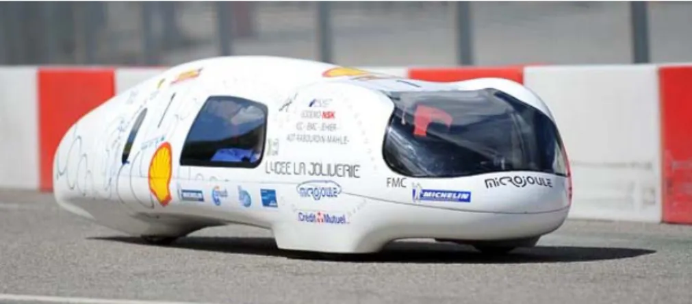
With 21 victories on the annual event, Microjoule from La Joliverie team is “the team to beat in the Prototype petrol category” [25] (see Figure 2.16). In 2009 they won the SEM 2009 Europe edition, with a consumption of 37771 / . The vehicle as a body shape similar to a water droplet, with the wheels completely embedded on the bodywork. This concept reduces the

(43)

19 ground clearance to the most and provides a low frontal area, approximately 0.31 . It is also possible to see that the top has a small curvature to reduce the downforce effect, achieving a drag coefficient of 0.1 [26].

Figure 2.16 - Microjoule from La Joliverie team

Another good reference is the Fancy Carol prototype fuel vehicle, from Japan (see Figure 2.17). With a totally different vehicle body shape, the Fancy Carol won in 2004 a world record during a SEM United Kingdom event, with a consumption of 3963 / [27]. This vehicle adopted a constant ground clearance all over the under body to reduce the suction effect and so the downforce. The wheels are also totally covered reducing the drag area by 12%. Another particularity is the minimization of the vehicle’s size and frontal area, which are important to reduce the drag value. These concepts leads to a vehicle with a frontal area of 0.21 and a drag coefficient of 0.12 at 70 / [2].

(44)

20

Despite of the lack of specific literature covering SEM vehicles aerodynamics, it was possible to deduce some important factors common on prototype vehicles that have a huge impact on vehicle performance. These factors must be taken in account when designing a prototype vehicle. The most important factors are the following ones:

 Low frontal area;

 Top body curvature (reducing downforce and so reduce drag coefficient);  Laminar flow extension;

 Wheels fairing;  Body angle of attack.

(45)

21

Chapter 3

3. Methodology

This chapter describes the process of AERO@UBI vehicle body design, the mesh generation process and the solution options used for the simulations. Therefore, initially this chapter will present the concept used to create the body geometry, the process of design in CATIA V5R20 and an improvement of the first design, later performed in Blender 2.73. In this chapter it is also introduced the use of the XFLR5 software in the process. In a second section, the CDF mesh generation with HELYX-OS software on Ubuntu is presented, followed by the explanation on the use of ANSYS Fluent as the solver.

3.1 Aerodynamic Design of the Vehicle

3.1.1 Design Concepts

Like the other SEM vehicles in competition, the principal objective on the design of the body is the minimization of the drag force. For that, it exists a wide range of solution concepts from the minimization of the frontal area to the use of certain body shapes, like those presented in Chapter 2.

From a long time ago that the dolphins and whales are subjects of aerodynamic studies. There are many references that describe the dolphins’ bodies as being related to modern low drag laminar flow airfoils [28] [29]. There are also studies to recreate the whales’ fins planforms for airplane wings. Galvão [1] wrote a paper about the similarity of the shark body shapes and airfoils. He discovered that their body is like a laminar flow symmetric airfoil with its thickness altered to exaggerate the airfoil section shape and he gave mathematic proof. With that he proposed a relation between a 2D airfoil and a 3D revolution body that will have the same pressure coefficient distribution along the longitudinal axis. In this way it is possible to minimize the drag of a fuselage using widely available airfoil data. The relation he came up with can be characterized by the equation (3.1). In Figure 3.1 it can be seen the visual representation of the application of the equation for the symmetric airfoil NACA 0012.

(46)

22 where,

⁄ – Dimensionless horizontal position of the airfoil

– Dimensionless horizontal position of the revolution body – Dimensionless radius of the revolution body at position

– Dimensionless vertical coordinate of the airfoil at position ⁄

Figure 3.1 - NACA 0012 transformation by equation (3.1)

A second concept was introduced for the vehicle body design, the equivalent body of revolution. This concept is based on the transonic equivalence rule, which states that the flow far away from a slender body becomes axisymmetric and equal to the flow around an equivalent equal cross-sectional area body of revolution [30]. This concept will allow the new body have the same pressure coefficient distribution along the longitudinal axis as the body of revolution created by the transformed airfoil. With these two concepts it was possible to create a procedure for the creation of the present vehicle body:

1. An initial vehicle design mainly based on ergonomics to evaluate the internal volume needed for the pilot and other systems;

2. Analyze the radius distribution of the first body considering the equivalent body of revolution concept;

3. Select an appropriate airfoil;

4. Apply the geometric transformation (3.1) to the created airfoil;

5. Check if the transformed airfoil satisfies the required internal volume radius distribution;

6. Divide the body of revolution in sections along the longitudinal axis;

7. Adapt each section shape along the longitudinal axis according to internal volume necessity, in the corresponding longitudinal position, keeping the same section area value to satisfy the equivalent body of revolution concept.

0 0,02 0,04 0,06 0,08 0,1 0,12 0,14 0,16 0 0,1 0,2 0,3 0,4 0,5 0,6 0,7 0,8 0,9 1 y/c y/l x/c x/l N0012 N0012 transformed r y

(47)

23 In sum, the design consists in the replication of the pressure coefficient distribution of an airfoil with late boundary layer transition point to have a lower drag. With the transformation applied to the airfoil, it is created a 3D body of revolution. From the later, comes the creation of the new body adapted to the internal volume shape, but respecting each equivalent section area of the body of revolution.

Figure 3.2 - Flowchart of implemented concept

3.1.1.1 Concept evaluation

The first equation determined by Galvão [1] is shown on equation (3.2). As it can be seen the only difference is the value of the exponent, increasing from 1.17 to 1.5. Galvão [1] explained that this change is due to have a better approximation of the velocity gradient. This change rises a question though, what is the effect on pressure distribution on the 3D body surface? To answer that, multiple simulations were performed on revolutions bodies generated with different exponentials values to study the behavior of the pressure distribution and find the most appropriate exponent to use for the transformation of airfoils into bodies of revolution.

100 ∙ 100 ∙ . (3.2)

To have a better perception of the influence of the exponent value, the simulations were run without the ground wall condition to be more similar to the airfoil flow condition. However these simulations were performed after the construction of the vehicle due to the tight deadline for the competition. That means the vehicle was designed with the equation (3.1), and all the conclusions of the exponential value influence analysis will be available for implementation in future works on the vehicle body development.

3.1.2 Concept Implementation

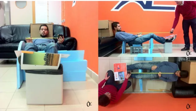
In a first stage it was necessary to define the pilot position based on a good ergonomic position and also on the SEM 2014 rules [31], such as the visibility requirements. For that, the driver position was studied and implemented (see Figure 3.3).

Note that, at that time, the team pilot was quite a big person for the job, 1.69 tall, compared with the typical top team pilot. This fact contradicted a fundamental design concept that it is usually present in any good aeronautical engineering design: the best streamlined shape body can be even better if made smaller, it will have even smaller drag.

(48)

24

Figure 3.3 – 3 Views of pilot position a) Front view b) Side View c) Top View

With the pilot position defined in 3 views it was possible to export the driver position to CATIAV5R20 and start the first vehicle design stage. This first design was created to evaluate the space needed and study the placement of the various internal components, e.g. the wheels, which in this case were two front steering wheels and one propulsive rear wheel. It were also followed the SEM 2014 rules, where on Chapter 1 article 39 they dictate the limits of dimensions for the vehicle body [31]. This tadpole vehicle configuration was later changed to tricycle for implementation of an innovative vehicle tilting steering system to eliminate tire cornering drag. This limitations can be consulted on Appendix A - Table A.1. Like shown in Figure 3.4 and Figure 3.5, the initial vehicle design shows the effort of reducing the size while respecting the basic principles of streamlined vehicle aerodynamics in preventing any boundary layer separation, above all, eliminate bluntness in the after body shape.

Figure 3.4 - 3D view of first design of the vehicle configuration concept

a)

b)

(49)

25

Figure 3.5 - 3 Views of first design of the vehicle configuration concept. Dimensions in [mm] a) Front View b) Side View c) Top View

The next step was to evaluate the cross section area distribution along the longitudinal axis of this initial body design. For that, a series of transversal planes separated of 10mm along the longitudinal axis. As each plane was created, the vehicle was cut by it to create transversal cross sections (see Figure 3.6).

Figure 3.6 - Example of transversal section

Each cross section has an associated area calculated with the CATIA V5 Measure Item tool. In order to compare the vehicle cross section area distribution to that of an airfoil, it was defined the equivalent body of revolution of the initial body by using equation (3.3) to calculate each cross section radius.

a)

b)

(50)

26 0 60 120 180 240 300 0 200 400 600 800 1000 1200 1400 1600 1800 2000 2200 2400 rcar [mm] x [mm]

Figure 3.7 – Equivalent body of revolution of the initial design

(3.3)

where,

– Section radius

– Transversal area of the section obtained with CATIAV5

With this data the graphic on Figure 3.7 was constructed, which represent the equivalent body of revolution corresponding to the initial body design. Note that the effort to produce an initial streamlined design is not so clear in the body of revolution as it was (compare with Figure 3.5). With the required equivalent body of revolution to satisfy the internet volume needs it was possible to search for the suitable airfoil to match the overall required radius distribution of the vehicle.

3.1.2.1 Airfoil Selection

The airfoil selection was constrained by the following criteria:  Symmetric Airfoil;

 Low drag value;  Low friction value;

 Good pressure distribution with late transition.

If Galvão’s theory is right [1], it will be possible to maintain the airfoil properties for the new design 3D body of revolution. To begin the airfoil selection, it is necessary to calculate the Reynolds number where the vehicle will operate, equation (3.4), in order to have a design point.

(51)

27 ∙ ∙ _(3.4) Where: – Reynolds number - Vehicle velocity ⁄ – Vehicle length – Dynamic viscosity ∙ ⁄

To define it is necessary to follow SEM rules. On chapter 2 of official SEM rules under article 123 [32] it is said: “For their attempt to be validated, teams must complete ten laps in a maximum time of 39 minutes with an average speed of approximately 25 km/h.” [32].It is also important to define the allowed length interval for the vehicle’s body. For that, it was defined 2200 as the minimum length, which is an approximated length of the initial design and 3500 for the maximum length, which is the maximum length permitted by the rules. In Table 3.1 the data used to calculate the Reynolds range for the vehicle is shown.

Table 3.1 - Data for the calculation of the vehicles body Reynolds number

25 ⁄ ≅ 7 ⁄

2200 2.2

3500 3.5

1.225 ⁄ 1.827 10 ∙ ⁄ With this data the new body Reynolds number range is:

1024372; 1629682

After defining the Reynolds range it is possible to start the study of multiple symmetric airfoils. For that, an analysis tool was used that can analyze airfoils that operate at low Reynolds numbers. The tool was XFOIL [33] through XFLR5 [34] interface. XFOIL is a proven airfoil design and analysis tool [35].

To start an analysis it is necessary to input the airfoil coordinates on the software via DAT files. Those airfoil files can be consulted and downloaded at the UIUC Airfoil Data Site [36]. The first selected airfoils were some well-known airfoils to see how they behave for our range of Reynolds and to check the coordinate distribution of those transformed airfoil with the radius distribution of the initial body vehicle design. However, since the vehicle configuration changed for one propulsive front caster wheel and two tilting rear wheels, it was decided to try the design of a new airfoil in order to get a lower drag coefficient, with an extensive laminar region and an appropriate transformed airfoil radius distribution. The cr001 airfoil was a start point to create a suitable airfoil, where the upper surface of airfoil was used to create the symmetric version of the airfoil. After loading the DAT file of the symmetric upper surface of cr001 on

(52)

28

XFLR5, the airfoil modification proceeded using the direct inverse design to change the pressure coefficient profile resulting in a changed thickness distribution, camber line and trailing edge thickness (see Figure 3.8).

After each modification of the airfoil a direct analysis was performed to compare the generated airfoil with the existing airfoils, to perform this analysis some parameters were defined to simulate the vehicle conditions. One of these parameters is the Reynolds number range who was already calculated, and the other is the turbulence level, NCrit [37]. It translate the freestream turbulence level effect on the boundary layer transition model, the lower is this number the higher is the effect of turbulence. The standard and commonly used value for this parameter is NCrit=9 (see Table 3.2), but for the present study case NCrit=2 was chosen to simulate the turbulence caused by the body surface imperfection and road induced vibration of the vehicle body. The analysis were ran with fixed airspeed and within a small angle of attack range. The process of modifying the airfoil and checking the respective transformation into a revolution body against the required internal volume of the initial design continued iteratively until a satisfactory solution was found.

Table 3.2 - Typical values of NCrit for various situations [37]

Situation NCrit Sailplane 12-14 Motor glider 11-13 Clean wind tunnel 10-12 Average wind tunnel 9

Dirty wind tunnel 4-8

Figure 3.8 – Airfoil created on XFLR5 for the vehicle design

To validate the airfoil other airfoil were also analyzed with thick trailing edge and thickness modifications. The thick trailing edge was found to be a compromise in terms of drag increment and suitability of the transformed airfoil to the required cross section area distribution of the initially designed body. In graphic of Figure 3.9, the drag coefficient is lower on final solution airfoil than the others, and also has a lower variation of the drag coefficient with the angle of attack, thereby achieving the goal of low drag. Figure 3.10 shows that AERO@UBI airfoil has a

(53)

29 larger laminar zone extension for higher angles of attack, despite the AH 79-100 A mod having a lower drag coefficient at 0° angle of attack. With the airfoil selected it is possible to apply the transformation to evaluate the cross section area distribution compatibility of the final revolution body versus the initial body design equivalent revolution body. In Figure 3.11 the transformed airfoil was translated to the left (moved forward of the initial design nose position) to have a better match in the cross section area distribution and it was also applied a thickness factor of 0.84 on vertical coordinate, modifying the thickness of the airfoil to better match the transformed airfoil cross section are distribution to that required by the initial body design. This transformations does not affect the properties of the airfoil, only the module of the pressure coefficient changes but not the drag characteristics. A flowchart of all the process of airfoil selection is shown on Appendix B - Figure B.1, giving a better understanding of the process.

Figure 3.9 - Variation of Drag coefficient with angle of attack3_Re=1500000

Figure 3.10 - Longitudinal position of the boundary layer transition3_Re=1500000

3_{Data extracted from XFLR5}

0 1 2 3 4 5 6 7 0,006 0,007 0,008 0,009 0,01 0,011 0,012 0,013 0,014 α [°] Cd AERO@UBI airfoil AH 79-100 A mod NACA 66-013 mod 0 1 2 3 4 5 6 0 0,1 0,2 0,3 0,4 0,5 0,6 0,7 0,8 0,9 1 α [°] Transition position x/c AERO@UBI airfoil AH 79-100 A mod NACA 66-013 mod

(54)

30

Figure 3.11 - Coordinate distribution

3.1.2.2 Vehicle Body Design

The objective of this method is to create a 3D body of revolution from the transformed selected airfoil and modify this body of revolution to a new 3D equivalent body adapted to the internal volume shape requirement by changing each cross section shape but maintaining the corresponding cross section area. To help the design of the vehicle body the first modification to the transformed airfoil 3D body of revolution was to camber the symmetry axis to better comply with the pilot position, while trying to end with a positive camber to prevent the generation of lift due to ground interference in the flow. By doing so, all cross sections continued to be circles. The created pseudo revolution body with a deformed axis is shown in Figure 3.12. This first shape helped to give a first idea of the final body shape and also served as a support to compare the cross section areas as each section was being changed to its convenient shape.

The final vehicle body shape was created with multiple cross sections spaced by 6 (see Figure 3.13) along the longitudinal axis since the actual construction of the vehicle body was made from 6 roofmate boards that were cut with a four axis CNC hot wire cutting machine and glued between them. The use of CATIAV5 Multi-Sections Surface tool gave a shape with some irregularities. This was mostly the result of iteratively changing each cross section shape while trying to respect the prescribed cross section area distribution. In the actual vehicle body, the final shape smoothing was performed with sand paper. To realize the CFD study, it was necessary to correct the shape. This was performed with another software: Blender. It is an open source 3D creation suite [38] commonly used by designers and movie industry but also used by engineers as a CAD tool to optimize the quality of surfaces. The shape was exported from CATIAV5R20 in STL format to Blender, and modifications were made to smooth the final body surface to get as close as possible to the actual prototype (see Figure 3.14).

0 50 100 150 200 250 300 350 -200 0 200 400 600 800 1000 1200 1400 1600 1800 2000 2200 2400 R [mm] x [mm] AERO@UBI AERO@UBI airfoil

(55)

31

Figure 3.12 - Lateral view of asymmetric body created for support design

Figure 3.13 - Multiple section sketch of AERO@UBI

(56)

32

For this project it was necessary to exclude the wheels and their cavities due to the high mesh complexity that would result and the available computational resources. With that, some modifications on vehicle shape to be possible to make a CFD simulation, these modifications consisted mainly on closing the wheels cavities (see Figure 3.15). On future works it advised to simulate a single wheel with a cavity, or even the whole assembly, to evaluate the impact on vehicle aerodynamics performance.

Figure 3.15 - Closed cavities for CFD simulation

With the final body design it was evaluate once again the coordinate distribution. As it is possible to see in Figure 3.16 the distribution of the present body vehicle is almost equal to the transformed airfoil. The comparison with the actual prototype was not performed

Figure 3.16 - Final coordinate distribution of the vehicle

0 50 100 150 200 250 300 350 0 200 400 600 800 1000 1200 1400 1600 1800 2000 2200 2400 r [mm] ; y [mm] x [mm] ; c [mm] AERO@UBI AERO@UBI transformed airfoil

(57)

33

3.2 Grid Generation

For this simulation the mesh was created with the HELYX-OS software. This software is an open source Graphical User Interface (GUI) with the OpenFOAM developed by Engys [39]. Using HELYX-OS a basic mesh is created and the software controls snappyHexMesh, an advanced meshing tool of OpenFOAM which is able to mesh the geometry from STL files [40]. Andrew Jackson on 7th_{OpenFOAM workshop 2012 gave a good explanation about the parameters}

available on snappyHexMesh [41]. It would be possible to perform all the simulation using HELYX-OS and the OpenFOAM suit but it was opted to use ANSYS Fluent, as solver for the created mesh.

3.2.2 Grid Generation Process

The use of a suitable mesh for the CFD simulation is important in order to have a valid result. For that, the choice between a structured mesh and an unstructured mesh needs to be made. For a complex geometry an unstructured mesh is faster to create than a structured mesh. However the structured mesh results in a better algorithm to store data, adding/subtracting 1 from cell indices (see Figure 3.17), it have less computational memory storage demand and therefore lower convergence time [42]. Also, with a structured mesh it is possible to have the cell aligned with the flow, helping further on the convergence time.

Figure 3.17 - Structured mesh representation - , ⇐ data stored on a 2D array

One of the advantages of HELYX-OS is the simplicity of creating a structured mesh, where it is possible to add layers around the body to have a better mesh resolution within the boundary layer and also the possibility to refine the mesh on a desired region where intense gradients are expected.

Like explained in Section 2.2.4, in order to have a valid result, the blockage ratio should to be lower than 7.5%. For that it is necessary to give suitable dimensions to the control volume. In Figure 3.18 it is shown how the control volume has been defined to minimize the blockage effect, where L is the vehicle’s length.

(58)

34

Figure 3.18 - Dimensions for control volume (half body) and boundary mesh labels

With the control volume defined the next step is the creation of the mesh in HELYX-OS. The first step in HELYX-OS is the creation of the control volume bounding box. In Figure 3.19 it is shown how this box is defined in the software, where all the values have as origin the origin of the CATIAV5 design.

Figure 3.19 - Bounding box definition

To have a better mesh it is recommended to create a mesh where cells are perfect cubes, equation (3.5) demonstrate how the number of elements was calculated to have the same cell size in each axis. This is criteria used to create the basic mesh.

| | | | | | _(3.5)

where,

, and – maximum distance from the references plans for each axis , and – minimum distance from the references plans for each axis , and – number of elements for each axis

2L 2L L 4L L Inlet Outlet Top Symmetry Ground Side