BJRS
RADIATION SCIENCES
07-02B (2019) 01-18ISSN: 2319-0612 Accepted: 2019-07-09
A comparative study of boron transport models in NRC
thermal-hydraulic code TRACE
N. Olmo-Juan
a, T. Barrachina
a, R. Miró
a, G. Verdú
a, C. Pereira
ba Institute for Industrial, Radiophysical and Environmental Safety (ISIRYM), Universitat Politècnica de València, Camí
de Vera s/n, 46021, València, Spain
b Departamento de Engenharia Nuclear, Universidade Federal de Minas Gerais, Av. Contorno, 842/9° andar, Centro,
30110-060 Belo Horizonte, MG, Brasil [email protected], [email protected]
ABSTRACT
Recently, the interest in the study of various types of transients involving changes in the boron concentration inside the reactor, has led to an increase in the interest of developing and studying new models and tools that allow a correct study of boron transport. Therefore, a significant variety of different boron transport models and spatial difference schemes are available in the thermal-hydraulic codes. According to this interest, in this work it will be compared the results obtained using the different boron transport models implemented in the NRC thermal-hydraulic code TRACE. To do this, a set of models has been created using the different options and configurations that could have influence in boron transport. These models allow us to reproduce a simple event of filling or emptying the boron concentration in a long pipe. Moreover, with the aim to compare the differences obtained when one-dimensional or three-dimensional components are chosen, it has modeled many different cases using only pipe components or a mix of pipe and vessel components. In addition, the influence of the void fraction in the boron transport has been studied and compared under close conditions to a BWR com-mercial model. A final collection of the different cases and boron transport models are compared between them and those corresponding to the analytical solution provided by the Burgers equation. From this comparison, important conclusions are drawn that will be the basis of modeling the boron transport in TRACE adequately.
1. INTRODUCTION
The importance of the accuracy in the simulation of boron transport in nuclear reactor lies on the fact that boron dilution have a great importance in order to manage the reactivity control, together to the movement of the control rods, in pressurized water reactors (PWR) and to maintain the core integrity during ATWS-kind severe accidents, in boiling water reactor (BWR) in which under certain circum-stances a boron injection is required.
Recently the interest in developing suitable tools that allow the reproduction of various types of tran-sients involving the variation of the boron concentration inside the reactor [1] has led to an increase of the studies of new models and numeric schemes and its accuracy.
In first order numeric schemes the process of discretization of mass and energy equations involves the introduction of numerical diffusion that avoids performing high accuracy simulations [2]. To min-imize numerical diffusion different high order schemes have been developed. Nevertheless, some second order schemes are not reliable since they can produce non-real oscillations.
In safety analyses, thermal-hydraulic calculations have to be accurate and reliable; they have to be able to reproduce real transients always with the same prediction. And in the case of transients in-volving a dilution or an injection of boron it is crucial to be able to simulate the boron transport within each component of the model.
Following this line of interest, the aim of this paper is to test the thermal-hydraulic code TRACE to simulate the boron transport with the different second order schemes that it has in the βeta version. For this, a set of models in TRACE using 1D and 3D components, under single-phase and two phase thermal-hydraulic conditions, is done and the results are compared to the analytical solution provided by the Burgers equation.
The paper is organized as follows: Section 2 is devoted to explain the basis of the different schemes implemented in TRACE and the Burgers equation. Section 3 explains the models and transients used to test the different schemes. The results and discussions are in Section 4. And finally, Section 5 summarizes the main conclusions of this work.
2. BASICS OF THE SCHEMES ANALYZED
2.1. First order and second order schemes.
In TRACE [3] there are 4 different second order schemes [4] implemented in the βeta version for the resolution of the diffusion term of the equations: MUSCL [5], Van Leer [6], OSPRE [7] and ENO [8]. In this section, a brief review of these methods and the first order upwind method is presented to show the basics of each one of them.
The expressions are developed to the boron density calculation, which is the goal of this work. Let’s start with the solute mass conservation equation:
𝜕[(1 − 𝛼)𝜌ℓ𝐶𝑏]
𝜕𝑡 + ∇[(1 − 𝛼)𝜌ℓ𝐶𝑏𝑣⃗ℓ]= 𝑆 (1)
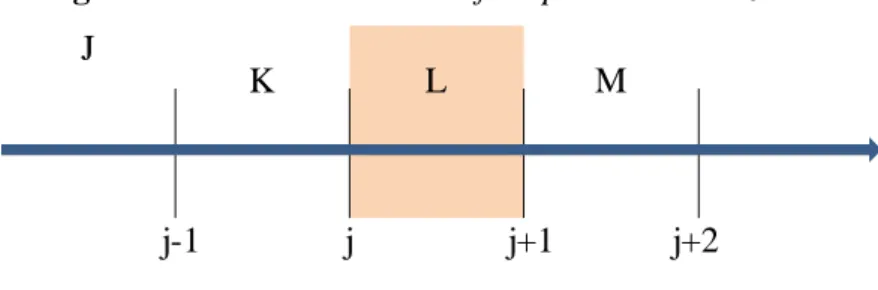
The nomenclature used for the spatial discretization is shown in Figure 1.
Figure 1: Nomenclature used for spatial discretization J
K L M
j-1 j j+1 j+2
For the semi-implicit temporal integration method the equation is:
[(1 − 𝛼)𝜌ℓ𝐶𝑏]𝐿𝑛+1−[(1 − 𝛼)𝜌ℓ𝐶𝑏]𝐿𝑛
∆𝑡 + ∇𝑗[((1 − 𝛼)𝜌ℓ𝐶𝑏)
𝑛
Despite the fact that the first term of the equation is similar for all the schemes, the second term is defined in different way for each scheme. It should be noted that the study has not considered the possibility that the solute precipitate so it is not taken into account in equations.
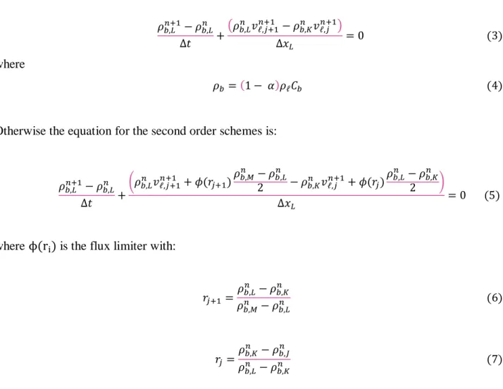
In case of the first order upwind scheme we have:
𝜌𝑏,𝐿𝑛+1− 𝜌𝑏,𝐿𝑛 ∆𝑡 + (𝜌𝑏,𝐿𝑛 𝑣ℓ,𝑗+1𝑛+1 − 𝜌𝑏,𝐾𝑛 𝑣ℓ,𝑗𝑛+1) ∆𝑥𝐿 = 0 (3) where 𝜌𝑏=(1 − 𝛼)𝜌ℓ𝐶𝑏 (4)
Otherwise the equation for the second order schemes is:
𝜌𝑏,𝐿𝑛+1− 𝜌 𝑏,𝐿𝑛 ∆𝑡 + (𝜌𝑏,𝐿𝑛 𝑣 ℓ,𝑗+1𝑛+1 + 𝜙(𝑟𝑗+1) 𝜌𝑏,𝑀𝑛 − 𝜌 𝑏,𝐿𝑛 2 − 𝜌𝑏,𝐾𝑛 𝑣ℓ,𝑗𝑛+1+ 𝜙(𝑟𝑗) 𝜌𝑏,𝐿𝑛 − 𝜌 𝑏,𝐾𝑛 2 ) ∆𝑥𝐿 = 0 (5)
where ϕ(ri) is the flux limiter with:
𝑟𝑗+1= 𝜌𝑏,𝐿𝑛 − 𝜌𝑏,𝐾𝑛 𝜌𝑏,𝑀𝑛 − 𝜌 𝑏,𝐿𝑛 (6) 𝑟𝑗= 𝜌𝑏,𝐾𝑛 − 𝜌𝑏,𝐽𝑛 𝜌𝑏,𝐿𝑛 − 𝜌𝑏,𝐾𝑛 (7)
The flux limiter ϕ(ri) present in equations is a nonlinear function that takes different expressions according to the chosen second order schemes. In Table 1 the flux limiter of each of the schemes analyzed are presented.
Table 1: Flux limiters
Scheme 𝜙(𝑟𝑖)
Van Leer (r + |r|)/(1 + |r|)
ENO Max[0, min(r, 1)]
OSPRE 1.5(r2 + r)/(r2 + r + 1)
2.2. Analytical Solution of Linearized Burgers Equation.
The linearized Burgers equation [9] is:
𝜕𝜌𝑏 𝜕𝑡 + 𝜕(𝜌𝑏𝑣𝑏) 𝜕𝑥 = 𝜕 𝜕𝑥(𝐷 𝜕𝜌𝑏 𝜕𝑥)+ 𝑆 (8)
Equation (8) has an analytical solution that allows evaluating the accuracy of the different first order and second order schemes described above. The time-dependent boundary condition is a Heaviside function, or step function, applied at the pipe inlet. The initial conditions for the analytical test are:
Emptying initial conditions:
𝐶(𝑥, 0)={𝐶0 , 𝑖𝑓 𝑥 ≤ 00 , 𝑖𝑓 𝑥 > 0
The above function practically represents the transport of a boron front diluted in water assuming that the void fraction is constant in the channel. Considering that the wave moves at velocity 𝑣 = 𝑣𝑓, no boron is generated inside the pipe 𝑆 = 0 and making the variable change 𝑧 = 𝑥 − 𝑣𝑓𝑡 (therefore, the observer stands at the center of the wave), equation (8) can be rewritten as:
𝜕𝐶 𝜕𝑡 = 𝐷
𝜕2𝐶
𝜕𝑧2 (9)
Equation (9) is a diffusion equation, which has a known solution. Therefore, the exact solution of equation (9) for the case of simulation of an emptying pipe is:
𝐶(𝑥, 𝑡)=𝐶0
2 [1 − 𝑒𝑟𝑓( 𝑣𝑡 − 𝑥
2√𝐷𝑡)] (10)
For the analogous case of filling, the initial conditions and the analytical solution would be:
Filling initial conditions:
𝐶(𝑥, 0)={0 , 𝑖𝑓 𝑥 > 0 𝐶0 , 𝑖𝑓 𝑥 ≤ 0 𝐶(𝑥, 𝑡)=𝐶0 2 [1 − 𝑒𝑟𝑓𝑐( 𝑣𝑡 − 𝑥 2√𝐷𝑡)] (11)
3. ANALYSIS OF THE BORON TRANSPORT MODELS IN TRACE
3.1. Models in TRACE
The study of the capabilities in TRACE for tracking the boron transport is based on the analysis of various simulations considering the use of 1D and 3D components as well as single-phase and two-phase thermal-hydraulic conditions. The aim of this work is to analyze a boron injection and a dilution in all the cases considered from a steady-state condition.
The 1D model consists of a long pipe with boundary conditions at the inlet and at the outlet. Two models have been tested: horizontal and vertical pipe.
In both models, the pipe has a length of 60 meters and it is divided in 99 cells with a uniform area of 50 cm2. Moreover, with the aim of studying the influence of the void fraction in the boron tracking, two different thermal-hydraulic conditions have been implemented, as it is presented in table 2. Thus, in the first of them a subcooled liquid condition, at 350 K (76.85 ºC) and 43 bar, very far from its saturation temperature, is studied. On the other hand, a saturated two-phase fluid condition at 69.9 bar (closely to the pressure inside a nuclear reactor in a BWR) and a inlet void fraction of 0.5 is
chosen to reproduce the same set of simulations. In this case, the saturation temperature is 558.882 K.
Table 2: Thermal-hydraulic properties of the single-phase and two-phase fluid
Single-phase conditions Two-phase conditions
Inlet boundary conditions Inlet boundary conditions
Velocity: v = 1 m/s Void fraction: α = 0.5
Temperature: T = 350 K Temperature: T = 558.882 K Outlet boundary conditions Outlet boundary conditions
Pressure: P = 43 bar Pressure: P = 69.9 bar
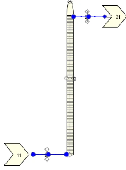
The 3D models are based on the unique 3D component in TRACE: the vessel. Thus, it has been done a VESSEL component equivalent to the 1D component. That is, a long VESSEL with 99 axial cells and only one radial and azimuthal sectors, respectively. The boundary conditions applied are the same as the 1D models. Like in the 1D models, we have tested the horizontal and the vertical vessel in a dilution and in an injection of boron.
In the 3D models, there are PIPE components that connect the VESSEL to the boundary conditions (FILL and BREAK components). The reason for this addition is that a VESSEL component cannot be directly connected to a BREAK component, so a single PIPE of the same dimensions as the BREAK is interposed between them. On the other hand, the second PIPE must be added between FILL and VESSEL components because it was observed that boron is not transmitted from the FILL to the rest of the system if a PIPE is not used to connect it to the VESSEL. In order to avoid that the presence of this PIPE at inlet affect the study of the 3D component, the pipe length considered is 1 millimeter and the flow area is the same as the vessel component.
It should be noticed that the possibility to use a vessel component in horizontal position is not possible in TRACE so it has been done an approximation by modifying the direction of the gravitational force in order to obtain a pseudo-horizontal vessel.
Figure 2: Model implemented in TRACE using tridimensional components
The aim of this model is to analyze if the boron tracking in the tridimensional components is done correctly, as well as to analyze the possible variations that could be generated by the different joints between components. Especially in the case where exists two-phase fluid conditions in the system. In all the models two transients are simulated. In the first one, a mass concentration of 2000 ppm of boron is injected from steady state conditions without any presence of boron. In the second transient a dilution is simulated. Starting with a mass concentration of 2000 ppm, pure water is introduced in the system in order to dilute the initial boron mass concentration.
Table 3: Description of the simulated transient
Filling model Emptying model
𝑡 < 0 → 𝐶𝑏 = 0 𝑝𝑝𝑚 𝑡 < 0 → 𝐶𝑏 = 2000 𝑝𝑝𝑚 𝑡 = 0 → 𝐶𝑏 = 2000 𝑝𝑝𝑚 𝑡 = 0 → 𝐶𝑏 = 0 𝑝𝑝𝑚
The simulated transient lasts 100 seconds and the results are shown for the center cell of the pipe (the 50th of 99 cells) which allows evaluating the boron front at this point.
To sum up, four models in TRACE has been created in order to simulate four different cases each one. Thus, we have the following list of cases:
Table 4: Summary of the simulations considered
Models in TRACE Different cases
Horizontal PIPE Single-phase filling
Vertical PIPE Two-phase filling
Horizontal VESSEL Single-phase emptying
Vertical VESSEL Two-phase emptying
3.2. Parameters in TRACE for simulating the boron tracking
According to the available specifications in TRACE concerning the tracking of the boron concentra-tion, the following variables have been explored:
• NAMELIST VARIABLES
- ISOLCN: In all the cases, it is activated with a value equal to 0. This option allows modifying the characteristic solubility of the specified solute. If “0” option is selected, it has been used the default solubility curve. It is noteworthy that this table only spec-ifies the solubility of boron in water with temperature, there being no temperature values beyond 110 °C, that is, quite far from the temperature of the simulated cases. Despite of this, the low concentration of boron used (2000 ppm) is far from the max-imum solubility considered, leaving out the possibility that the solute precipitates. So that option is not really interesting in our simulations. The other options refer to the possibility of modifying the solubility curve and how to specify it as a table, function, etc.
- FRACB10: Its use refers to the calculation of the reactivity due to the variation of boron concentration in the system, and since there is no neutron process in the simu-lation performed, its use has been considered unnecessary.
- ISOLUT: Available from the SNAP/TRACE Model Options menu, it is also called Solute Tracking. It has three different options, "0" in case you do not want to follow the boron, "1" if you want to follow but without recalculating the density of the sol-vent-solute mixture and "2" for those cases where the concentration of solute could be so considerable that the density of the mixture should be recalculated. This last option
is not available since SNAP menu. Moreover, some tests have been done trying to choose the “2” option, using the input file of TRACE, but it does not work with the executable used (TRACE patch 4). So, for the cases studied, the option "1" is chosen. - MAXCONC: This option is recommended for determining a convergence limit in the calculation of the precipitated solute. Its use is only needed in case the value of the selected ISOLUT variable is greater than the unit.
• VESSEL
- ICONC: This option is specified in the menu corresponding to the component "VES-SEL". It is also specified as a Solute Option and has three different options: "0" if no solute is contemplated in the liquid, "1" if it is contemplated, but without considering precipitation and "2", if it could be dissolved and precipitate solute. Since the boron concentration considered is clearly far of the maximum solubility, the “1” option is selected.
4. RESULTS AND DISCUSSION
In this section, the results obtained in the different simulations are presented. Along the various fig-ures presented below, the evolution of the boron concentration acquired for the different models in TRACE and the numeric schemes explained in the previous sections are shown. In all the cases, this evolution tried to reproduce a step input increasing or decreasing the boron concentration.
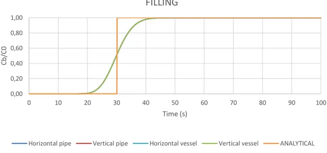
The results obtained in the case of boron injection and dilution under thermal-hydraulic boundary conditions of single-phase liquid, are shown in Figures 3 and 4. It is easy to appreciate that no differ-ences exist among the different configuration modelled in TRACE for the first order Upwind. Fur-thermore, it can be noticed that the moment, when the front evolution predicted by TRACE changes, is close to the analytical solution, but the way in wich is represented the step entrance is clearly inadequate.
Figure 3: Results of TRACE using Upwind solution for the single-phase filling and the analytical solution
Figure 4: Results of TRACE using Upwind solution for the single-phase emptying and the analyti-cal solution 0,00 0,20 0,40 0,60 0,80 1,00 0 10 20 30 40 50 60 70 80 90 100 C b/ C 0 Time (s)
FILLING
Horizontal pipe Vertical pipe Horizontal vessel Vertical vessel ANALYTICAL
0,00 0,20 0,40 0,60 0,80 1,00 0 10 20 30 40 50 60 70 80 90 100 C b/ C 0 Time (s)
EMPTYING
With the aim to obtain a more reliable reproduction of the step input variation, it has been modified the numeric schemes chosen in TRACE simulations. Thus, first order upwind scheme, which is orig-inally working by defect, has been replaced by the second order schemes available in TRACE. The modification of this parameter is done since Namelist Variable menu, selecting different values for the SPACEDIF parameter. Moreover, if a second order scheme is chosen, the numeric method defined in parameter NOSETS must be semi-implicit.
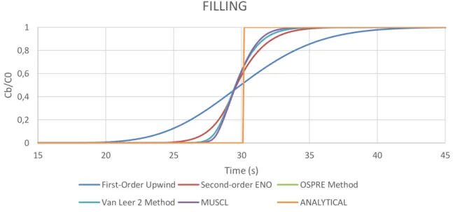
In figures 5 and 6 are shown the results of TRACE simulations using different numeric schemes in the case of a vertical vessel. As it was presented in the previous figures 3 and 4, the boron evolution under single-phase boundary conditions is similar in all the cases, so a vertical vessel has been se-lected for this comparison.
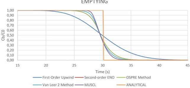
Five different numeric schemes have been compared and the results in both cases, filling and empty-ing, shows that the second order schemes present a more adequate step reproduction regarding the analytical solution, being the results of second order MUSCL scheme the most suitable. Besides, should be noted that the results obtained for Second-order ENO and OSPRE method are the same and the correspondent lines are overlapped.
Figure 5: Results of TRACE using different numeric schemes for the single-phase filling and the analytical solution 0 0,2 0,4 0,6 0,8 1 15 20 25 30 35 40 45 C b/ C 0 Time (s)
FILLING
First-Order Upwind Second-order ENO OSPRE Method
Figure 6: Results of TRACE using different numeric schemes for the single-phase emptying and the analytical solution
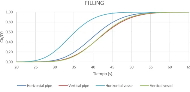
The results for boron injection and dilution under two-phase boundary condition are presented in figures 7 and 8. Contrarily to the equivalent results for the single-phase boundary condition simula-tion, it has been obtained big differences between some of the cases simulated. Thereby, the horizon-tal cases of pipe and vessel components shows a clear delay to the correspondent to their vertical options, which are quite close but not identical. This delay and the big delay that can be appreciated with respect to the previous cases are due to the existence of various void fraction in the steady state conditions. It should be also reminded that the analytical solution is only valid for the single-phase boundary conditions. 0,00 0,10 0,20 0,30 0,40 0,50 0,60 0,70 0,80 0,90 1,00 15 20 25 30 35 40 45 C b/ C 0 Time (s)
EMPTYING
First-Order Upwind Second-order ENO OSPRE Method
Figure 7: Results of TRACE using Upwind solution for the two-phase filling and the analytical so-lution
Figure 8: Results of TRACE using Upwind solution for the two-phase emptying and the analytical solution 0,00 0,20 0,40 0,60 0,80 1,00 20 25 30 35 40 45 50 55 60 65 C b/ C 0 Tiempo (s)
FILLING
Horizontal pipe Vertical pipe Horizontal vessel Vertical vessel
0,00 0,20 0,40 0,60 0,80 1,00 20 25 30 35 40 45 50 55 60 65 C b/ C 0 Tiempo (s)
EMPTYING
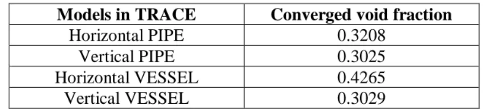
The values of the converged void fraction, presented in table 4, shown a great similarity between vertical pipe and vessel, and a small variance in the case of the horizontal pipe. However, big differ-ences exist in the case of the horizontal vessel. The fact of not using a real horizontal vessel, which is not implemented in TRACE, is considered an explanation for that big variance. As it was explained previously, we are considering a pseudo-horizontal vessel which is a vertical component with the gravitational force direction turned.
Table 4: Summary of the converged void fractions for the different models
Models in TRACE Converged void fraction
Horizontal PIPE 0.3208
Vertical PIPE 0.3025
Horizontal VESSEL 0.4265
Vertical VESSEL 0.3029
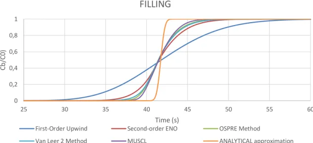
Finally, a comparison between the different numeric schemes in two-phase boundary conditions is shown in figures 9 and 10. The component chosen for this study is the vertical vessel that allows us to study a 3D component with a void fraction close to the correspondent to the 1D component. Fur-thermore, the analytical model used to solve the Burgers equation has suffered a modification for taking into account that the boron is only carried in the liquid phase, i.e. the boron is not dissolved in the vapour. For this reason, the area and the velocity of the analytical model has been modified for considering the converged values of the liquid phase as the input in the analytical model solved by Burgers equation.. As in the previous case, the second order MUSCL scheme is the option that allows a better reproduction of the step input boron evolution, Second-order ENO and OSPRE method show now dif-ferences and the evolution predicted by the first order Upwind method is clearly unsatisfying.
Figure 9: Results of TRACE using different numeric schemes for the two-phase filling and the approximation of the analytical solution
Figure 10: Results of TRACE using different numeric schemes for the two-phase emptying and the approximation of the analytical solution
0 0,2 0,4 0,6 0,8 1 25 30 35 40 45 50 55 60 C b/ C 0) Time (s)
FILLING
First-Order Upwind Second-order ENO OSPRE Method
Van Leer 2 Method MUSCL ANALYTICAL approximation
0,00 0,20 0,40 0,60 0,80 1,00 25 30 35 40 45 50 55 60 C b/ C 0 Time (s)
EMPTYING
First-Order Upwind Second-order ENO OSPRE Method
5. CONCLUSIONS
In the present work a set of models in TRACE have been modelled allowing to study the behavior of horizontal and vertical 1D and 3D components, under single-phase or two-phase thermal-hydraulic conditions and comparing the influence of the different numeric schemes, first and second order, available in TRACE.
The conclusions of this study is that first order Upwind scheme is not reliable for the transmission of a step input, like the most of events involving boron injection or dilution. Instead of this method, it is more suitable to use the second order MUSCL scheme, which is the closer scheme to the analytical solution, or its approximation, provided by the Burgers equation.
It has also been tested the boron evolution under two-phase boundary condition allowing to under-stand better the influence of the void fraction in the observed delay.
REFERENCES
[1] BARRACHINA T., SOLER A., OLMO-JUAN N., MIRÓ R., VERDÚ G. J., CONCEJAL A. Development of a high order boron transport scheme, In: JOINT INTERNATIONAL CONFER-ENCE ON MATHEMATICS AND COMPUTATION (M&C), SUPERCOMPUTING IN NU-CLEAR APPLICATIONS (SNA) AND THE MONTE CARLO (MC) METHOD, 2015, Nash-ville,TN, USA. CD-ROM, American Nuclear Society, LaGrange Park, IL (2015)
[2] OLMO-JUAN N., BARRACHINA T.M., MIRÓ R., QUEROL A., VERDÚ G.J., PEREIRA C.A comparative study of boron transport in thermal-hydraulic codes TRACE vs TRAC-BF1 and TRACE vs RELAP5, In: 17TH INTERNATIONAL TOPICAL MEETING ON NUCLEAR REACTOR THERMAL HYDRAULICS, 2017, Xi’an, China.
[3] U. S. Nuclear Regulatory Commission, TRACE V5.0 – Theory Manual, Washington, DC 20555 (2012).
[4] WANG, D.; MAHAFFY, JH.; STAUDENMEIER, J.; THURSTON, CG., Implementation and assessment of high-resolution numerical methods in TRACE, Nuclear Engineering anwhatd De-sign, 263, pp 327-341, 2013.
[5] VAN LEER, B.; Towards the ultimate conservative difference scheme. V. A second-order se-quel to Godunov’s method. Journal of Computational Physics 32, 101–136.
[6] VAN LEER, B.; Towards the ultimate conservative difference scheme II. Monotonicity and conservation combined in a second order scheme. Journal of Computational Physics 14 (4), 361– 370, 1974.
[7] N.P. WATERSON, H. DECONINCK. A unified approach to the design and application of
bounded higher-order convection schemes. In: 9TH INTERNATIONAL CONFERENCE ON NU-MERICAL METHODS IN LAMINAR AND TURBULENT FLOW, 1995, Taylor, Durbetaki (Eds.), Proceedings of the Ninth International Conference on Numerical Methods in Laminar and Turbulent Flow, Atlanta, July, 1995. Pineridge Press, Swansea, p. 203.
[8] SHU, C.W.; OSHER, S.; Efficient implementation of essentially non-oscillatory shock capturing scheme II. Journal of Computational Physics 83, 32–78, 1989.
[9] Burgers, J. M. The Nonlinear Diffusion Equation. D. Reidel Publishing Company, Dordrecht, Holland (1974).