Two phase flow models in DxUNSp code platform

Catalin NAE

*Corresponding author

INCAS - National Institute for Aerospace Research “Elie Carafoli”

B-dul Iuliu Maniu 220, Bucharest 061126, Romania

cnae@incas.ro

Abstract: The aim of this work is to find an efficient implementation for a two phase flow model in an existing URANS CFD code platform (DxUNSp), initially based on unsteady URANS equations with a k- turbulence model and various other extensions, ranging from a broad selection of wall laws up to a very efficient LES model. This code has the capability for development for nonreacting/reacting multifluid flows for research applications and is under continuous progress. It is intend to present mainly three aspects of this implementation for unstructured mesh based solvers, for high Reynolds compressible flows: the importance of the 5/7 equation model, performance with respect to a basic test cases and implementation details of the proposed schemes. From a numerical point of view, we propose a new approximation schemes of this system based on the VFRoe-ncv.

Key Words: CFD, two phase flows, URANS, Riemann solvers.

1. INTRODUCTION

As part of a continuous development effort for advanced numerical modeling methods and tools, INCAS has initiated for some time a development platform called DxUNSp ([1]). This platform has the capability to address a wide range of models and implementations, ranging from state-of-the-art URANS to LES, from single fluid to multi-fluid non/reacting flows, from local implementation to a high performance Grid environment. In this platform, a new extension is proposed for two-phase flow capability, as to be presented in this paper.

Modeling of two-phase flows is typically based on averaging procedures ([2],[3]). In their most general form, these averaging techniques produce models characterized by two different velocities and pressures for each phase supplemented by one or several topological equations.

Thus, in one dimension and for non-isentropic flows, a two-phase model of this type consists of at least 7 equations :

• two mass conservation equations, • two momentum equations, • two energy (or pressure) equations • one topological equation.

These type of models have been known for a long time ([15], [17], [7]) but have been seldom used due to their complexity.

However, some recent works [1] have shown that they possess several advantages over the more classical 6 equation system :

• these models are unconditionally hyperbolic,

• they are able to treat multiphase mixtures as well as interface problems between pure fluids

• they allow the treatment of fluids characterized by very different thermodynamics because each fluid uses its own equation of state.

However these models are numerically complex to solve because of the large number of waves they contain and of the sensibility of the results with respect to the relaxation procedures. These facts motivate the research of cheaper models and the present work.

2. UNIFIED FORMULATION FOR DXUNSP CODE

In the DxUNSp code, the set of Navier-Stokes equations and the constitutive relations are filtered in the physical space using a simple step decomposition based on a generic filter having the properties described in previous work [1].

The final version of the system is :





 









 













                            _{   }                            _{   }                          j t j ij ii ij j i j j ij ii ij t j i j i j i j j x k k x S S u x u e x e t S S x x u u x u t u x t ~ 3 2 ~ 2 ~ ~ ~ ~ ~ 3 2 ~ 2 ~ ~ ~ 0 ~            (1)

We intend to keep the same structure of an existing solver (RANS using 2 equation turbulence model) for the continuity, momentum end energy in order to induce a minimum of changes in the implemented version of the code.

The presented set of equations are for the single fluid case; details for the multi-fluid formulation will be presented later as a short comment.

Also, all new variables introduced by the LES approach are to be matched as close as possible to the existing ones.

This leads to a generalization of the pressure and temperature as macro parameters, depending on the SGS modeling.

The definitions and the constitutive relations used are (presented in an equivalent formulation to the classical RANS formalism):

kk ij ij ij j i i j ij S S P u x u x S ~ 3 2 ~ 2 ~ ~ ~ 2 1 ~                      ij SGS ij ij t ij kk ij ij ij ij j i j i ij p M D P M M T D T u u u u M                            2 3 1 ~ 3 1 ~ ~ (2) and i i v uu

C e R ~ ~ 2 1 ~_{ }     where ii v ii D C T D p  1 2 1 ~ 3 1     

 _and

t t p t p C k C k Pr Pr       (3)

It is a common practice to use the system as presented above, for compressible flows, with a general restriction for the Mach SGS number MSGS.

It is important to know when some SGS terms can be neglected and to have an indicator for these simplifications.

It is possible to show that Dij contribution can be neglected for low Mach compressible

flows and for monoatomic gases (where γ = 5/3), and with a certain error in all other cases, if the following criteria is satisfied:

0 0

6 5

3 _{    }

       ij SGS D M   (4)

The formal changes due to spatial filtering induced in the code structure are limited to a change in the effective viscosity term in the energy equation and we expect that turbulent viscosity t and turbulent Prandtl number Prt to be defined and computed using dedicated

routines.

3. THE 7 eg. MODEL

The starting point of this study is the seven equation model presented in [4] which is a slight variation of the Baer-Nunziato 1986 model [7]. In term of conservative variables, this model can be written as:













































                                                                       1 2 2 2 1 2 2 2 2 2 2 2 2 2 2 2 1 2 2 2 2 2 2 2 2 2 2 2 1 2 2 2 2 2 1 2 2 1 1 1 1 1 1 1 1 1 1 2 1 1 1 1 1 1 1 1 1 1 1 1 1 1 1 0 0 p p u t u u u t p u p e div t e u u p p u u div t u u div t u u u t p u p e div t e u u p p u u div t u u div t I I I I I I I                                        (5)

The notations are classical :

 αk are the volume fractions of each phase (α1 +α2 = 1),

 ρk the phase densities,

 uk the vector velocities,

 pk the pressures

 ek = εk+uk2/2 the specfic total energies

 εk the specific internal energies.

On the other hand, pI and uI stand for the interfacial pressure and velocity. In the Baer-Nunziato 1986 model [7], these variables are chosen as pI = p2 and uI = u1.





 

 ₂

2 2

2

k k k k

k k k I

u u

 

 

and



 

1

k k k

I p

p 

2

(6)

We note that the choice of interfacial velocity and pressure can have a deep impact on the structure of the waves present in this model and on the full development of entropy inequalities (see [9]).

However, in this paper as we will assume that the phase pressures and velocities relax to a common value, these choices are not important and will not affect the derivation of the reduced model.

4. THE 5 eg. MODEL

Actually, the model (5) contains relaxation parameters and > 0 that determine the rates at which the velocities and pressures of the two-phases reach equilibrium. The rationale for the introduction of such terms is discussed for instance in [4].

Here we are interested in situations where the relaxation times are small compared with the others characteristic times of the flow.

Thus we set :

= ’ / ε where ’ = O(1)

= ’ / ε where ’ = O(1) (7)

This analysis can be performed directly on the system (5) with the conservative variables (αkρk; αkρkuk, αkρkek α2)t.

We perform an asymptotic analysis for the case ε0 on this model in order to have an estimate on the terms of order ε.

After some algebraic manipulations, the model may be written in term of conservative variables (α1ρ1; α2ρ2, ρu, ρe,α2)t as :

















     

      

 

 

   

  

 

    

 

 

 

 

 





u a

a a u

t

u p e div t

e

p u u div t

u

u div t

u div t

k

k k k

div 0

0 0 0

2

1 2

2 2 2 2 1 1 2 2 2

2 2 2

2

1 1 1

1

 

     

 

 

  



  



(8)

Here the notations are:

 αk are the volume fractions of each phase (α1 +α2 = 1),

 ρk the phase densities,

 e = ε+uk2/2 the specfic total energies,

5. THE VFRoe-ncv SCHEME

In this section, we describe a quasi-conservative finite volume scheme. The method is based on VFRoe-ncv type scheme [8, 18] i.e on the solution of a linearized Riemann's problem at each interface of the mesh. We consider the following linearized Riemann's problem between the states (:)L and (:)R :

 

 

               0 x if 0 x if 0 , 0 R L q q x q t q q A t q (9)

Here, we use the set of variables q = t(s1; s2; vn; vt; p; Y2) where vn; vt are respectively

the two components of the vector velocity in the local basis (ηLR; ηtLR) where ηLR is the unit

normal vector to the interface. We define A(< q >) by :

 

                       n n n n n n v v a v v v v q A 0 0 0 0 0 0 ˆ 0 0 0 0 0 0 0 0 0 1 0 0 0 0 0 0 0 0 0 0 0 0 0 2   (10)

where < : >= ((:)L +(:)R)/2 denotes the arithmetic average between the states (:)L and (:)R.

The matrix A(< q >) is diagonalizable and the solution procedure reduces to the solving of a Riemann's problem for a linear hyperbolic system.

To deal with the non-conservative equation :

div 2 1 2 2 2 2 2 1 1 2 2 2



       k k k k a a a u

t _{ }

      (11)

we re-write it under the following form :

   

div 0

2   

 u Q B u div  2

t with

 



   ₂ 1 2 2 1 1 2 k k k k a a Q B     (12)

and we write the 5 eq. reduced model (8) like :

 

div

 

0

div  

   Q uB Q F t Q (13)

When we integrate on a cell Ci we find :

 

Q n dl B

 

Q u d i



N



F t Q A i i C C i

i _     div  0 for 1,...,









where N is the number of cells and Ai the area of cell Ci.

To update the Qi variable we use :





 



 

 

 

i v j

n j n i ij n

i n i

i n Q Q

t Q Q

A , 0

1

 (15)

where :

v(i) denote the set of cells Cj that share an edge with Ci

ij ij ij

C ij

n n n

dl n n

ij

 





 _{is the averaged normal vector of the interface:}

j i

ij

C

C

C











 

 



































 x

ij ij y ij ij ij

ij ij t

y ij ij x ij ij ij ij ij n

v

u

u

v

v

u

u

v













the normal and tangential components of

the velocity at the cell interface;

We propose the following expression for





Q_in,Qn_j



:



  

 

ij ij

n i ij

ij n

j n

i Q F Q BQ u

Q







 *   * 

, (16)

The conservative part F

 

Q_ij* 



_ij is then explicitly written :

 





 

 













 



*



2 * *

* *

* *

2 2 * 1 1 *

, ,

, ,

, n ij n _ij

y ij ij ij n x ij ij ij n ij n ij

n t ij

ij v v uv p vv p e pv v

Q

F                (17)

while the non-conservative part B

 

Q_in u_ij*



_{ij is defined by :}

 

*



 

 

*



, 0 , 0 , 0 , 0 ,

0 n _{n ij}

i t

ij ij n

i u BQ v

Q

B   (18)

It is also possible to show that the VFRoe-ncv scheme preserve an isolated contact discontinuity and that the velocity and the pressure must stay constant in this case.

Numerical experiment confirm that this is indeed the case except at very low Mach number.

This seems surprising because the analytic proof is independent of the Mach number. However, this proof assumes that the computations are done with exact arithmetic. In practice, this is not the case and round-off errors perturbate the computations.

6. VALIDATION TEST CASES

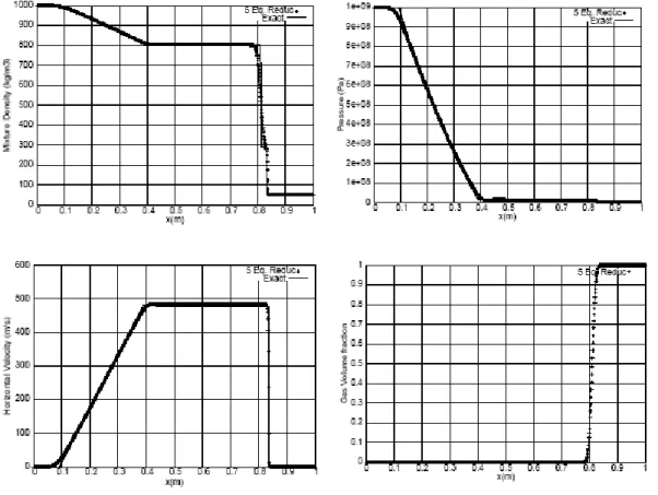
In order to validate the proposed 5eg. model, we consider a shock tube of one meter length filled on the left side (x < 0:7) with a high pressure liquid water and on the right side with air. This test problem consists of a classical shock tube with two fluids and admits an exact solution.

The state laws for the air and the water are given by the Stiffened-Gas formulation :

  

  

 

      

  

 

      

water 10

. 6 and

4 . 4 with

) 1 (

air 0

and 4

. 1 with

) 1 (

8 2

2 2

2 2 2 2

1 1

1 1 1 1 1

p p

The initial condition consists in a pressure discontinuity between p = 109 Pa in the liquid side and p = 105 Pa in the gas side.

The right and left chambers contain nearly pure fluids : the volume fraction of the gas in the water chamber is α1 = 10-8 and the fraction of water in the gas chamber is α2 = 10-8

(Figure 1).

Fig. 1 - The 5 eg. model for the water-air shock tube (mixture variables)

The second series of numerical experiments deals with two-phase flow and consider problems where the two phases are simultaneously present at the same location.

With this respect, the experiment considers the same problem than Test Case 1, except that the volume fraction is constant and equal to α1 = 0.5 everywhere in the domain for Test

On the left side (x < 0:5) the pressure is 109 Pa while it is equal to 105 Pa on the right side. The velocity is zero at time 0.

The discretization is done on a 1000 cells grid and the CFL number is fixed and equal to 0.6. The results are shown at time 200 s.

Fig.2 - The 5 eg. model for the two-phase flow problem

The results are in perfect agreement and this confirms that the present five equation model (5 eg.) is a correct asymptotic limit of the seven equation model in the limit of zero relaxation time.

In particular, we observe that even if the initial composition of the mixture is constant, it evolves in space and time and that this evolution is the same in the results obtained with the two models (Figure 2).

As a more complex test case, in Test Case 3 we present a series of numerical experiments by some relevant two-dimensional test-case.

This test shows the drop of a heavy bubble under the effect of the gravity in a closed box as described in Figure 3.

The box is one meter large and two meters high and the mesh is composed of 50 x 100 points.

These experiments are computed with a second order MUSCL technique for the space discretization.

Fig. 3 - Bubble drop test case – initial configuration

Although it seems simple, this computation presents several numerical difficulties. In particular, the Mach number in this computation is extremely low (it is equal to zero at time t=0 and increases slightly up to a value of 0.01 during computation).

Figure 4 shows the isovalues of the volume fraction at different times. Although an accurate simulation of this problem would require a finer mesh (or an adaptive procedure to follow the interface) the results are very promising.

In particular, the numerical diffusion do not prevent the development of interface instabilities and the volume fraction remains bounded

7. CONCLUSIONS

We have derived a five equation reduced model from an asymptotic analysis in the limit of zero relaxation time of a seven equation two velocity, two pressure model. Although, this model cannot be cast in conservative form, the mathematical structure of the model have been analyzed and shown to be very close to the structure of the Euler equations of fluid dynamics.

This model presents an interesting alternative to the use of the seven equation model: it is cheaper, simpler to implement and is easily extensible to an arbitrary number of materials.

From a numerical point of view, we have proposed new approximation schemes of this system. The VFRoe-ncv relies on an approximate linearized Riemann solver.

The numerical results show that the reduced five equation model is able of accurate computations of interface problems between compressible material as well as of some two-phase flow problems where pressure and velocity equilibrium between the two-phases is reached.

REFERENCES

[1] C. Nae, Unified formulation for URANS and LES in DxUNSp code, in INCAS Bulletin 1/2009, ISSN 2066- 8201.

[2] F. Coquel, J. M. Hérard, and N. Seguin, Closure laws for a two- uid two-pressure model. C. R. Acad. Sci. Paris, Ser. I 334:1-6, 2002.

[3] E. Godlewski and P. A. Raviart, Numerical Approximation for Hyperbolic systems of Conservation Laws. Spinger-Verlag, 1996.

[4] R. Abgrall and R. Saurel, A Multiphase Godunov Method for Compressible Multifluid and Multiphase Flows.

Journal of Computational Physics, 150, pp. 425-467, 1999.

[5] R. Abgrall and R. Saurel, A simple method for compressible multifluid flows. SIAM J. Sci. Comput., 21(3), pp. 1115-1145, 1999.

[6] G. Allaire, S. Clerc, and S. Kokh, A Five-Equation Model for the Simulation of Interfaces between Compressible Fluids. Journal of Computational Physics, 181, pp. 577-616, 2002.

[7] M. R. Baer and J. W. Nunziato, A two-phase mixture theory for the de agration-to-detonation transition (DDT) in reactive granular materials. Journal of Multiphase Flows, 12, pp. 861-889, 1986.

[8] T. Buffard, T. Galouët, and J. M. Hérard. A sequel to a Rough Godunov Scheme : Application to Real Gases.

Computers and Fluids, 29, pp. 673-709, 2000.

[9] D. A. Drew and S. L. Passman, Theory of Multicomponent Fluids., volume 135 of APPLIED MATHEMATICAL SCIENCES. Springer, New York, 1998.

[10] M. Ishii, Thermo-Fluid Dynamic Theory of Two-Phase Flow. Direction des études et recherches d’électricité de France. Eyrolles, 1975.

[11] A. K. Kapila, J. B. Bdzil, R. Meniko, S. F. Son and D. S. Stewart, Two-phase modelling of DDT in granular materials : reduced equations. Physics of Fluids, 13, pp. 3002-3024, 2001.

[12] M. H. Lallemand and R. Saurel, Pressure relaxation procedures for multiphase compressible Flows.

Technical Report 4038, INRIA, 2000.

[13] J. Massoni, R. Saurel, B. Nkonga and R. Abgrall, Propositions de méthodes et modèles Eulériens pour les problèmes à interfaces entre fluides compressibles en présence de transfert de chaleur. International Journal of Heat and Mass Transfer, 45 No 6, pp. 1287-1307, 2001.

[14] R. Natalini, Recent Mathematical Results on Hyperbolic Relaxation Problems. Analysis of systems of conservation laws, (Aachen, 1997), Chapman and Hall/CRC, Boca Raton, FL, pages 128 198, 1999. [15] V. H. Ransom and D. L Hicks, Hyperbolic Two-Pressure Models for Two Phase Flow. Journal of

Computational Physics, 53, pp.124-151, 1984.

[16] C. W Shu and S. Osher, Eficient Implementation of Essential Non oscillatory Shock capturing schemes.

Journal of Computational Physics, 77, pp. 439-471, 1998.

[17] H. B. Stewart and B. Wendro, Two-phase flow : Models and methods. Journal of Computational Physics,

56, pp. 363-409, 1984.