ISSN 2179-8087 (online)
Original Article
Forest Management
Creative Commons License. All the contents of this journal, except where otherwise noted, is licensed under a Creative Commons Attribution License.
Sampling Processes and Intensities for the Geostatistical
Modeling of an Unevenly Aged Forest
Marcelo Roveda
1
, Afonso Figueiredo Filho
2, Allan Pelissari
1
, Aline Genú
21Universidade Federal do Paraná – UFPR, Curitiba/PR, Brasil 2Universidade Estadual do Centro-Oeste – UNICENTRO, Irati/PR, Brasil
ABSTRACT
The aim of this study was to estimate the basal area, through traditional sampling processes and geostatistical interpolation, and compare it to the forest census carried out in 25 ha of a Mixed Ombrophilous Forest remnant. The sampling simulations were structured for the systematic sampling, two stages, and simple random, in intensities 5, 11, and 22% of the potential sample units of 25 × 25 m. The increase in sample intensity for the systematic sampling and two stages revealed a higher level of spatial behavior details of the basal area, whereas when comparing the census with sampling, it was observed that the geostatistical interpolation shows ability to improve the accuracy of the basal area estimation.
1. INTRODUCTION
Forest inventory has quantitative and qualitative information about forests (Campos & Leite, 2013). Regarding data collection, forest inventories can be classified into the total enumeration or census, in which all the individuals of the population are observed and measured, obtaining true values, while only a part of the population is observed for the sampling and an estimation of its parameters is obtained, which conveys an error (Péllico & Brena, 1997).
The process for performing the census of a forest is considered a time-consuming and onerous task (Machado & Figueiredo, 2006), hence the vast majority of forest inventories are carried out by sampling (Péllico & Brena, 1997). Thus, the sampling process and its sample intensity become the basis for estimating the characteristics of a population (Scolforo & Mello, 2006), and whose inadequate choice may underestimate or overestimate the forest interest variable (Corte et al., 2013).
Some researchers have evaluated and obtained some conclusions about different sampling processes and intensities in native forest inventories, such as Higuchi (1987) who observed that systematic sampling is more accurate than random sampling in commercial inventories in humid tropical rainforest on the mainland of Manaus; Ubialli et al. (2009) in an ecotonal forest in the northern region of Mato Grosso and Cavalcanti et al. (2009) in a native area located in the municipality of Sena Madureira in the Acre State, finding that the parcels/stands with the smallest error do not depend on the sampling process, while smaller errors were produced at higher sample intensities; and Corte et al. (2013) to express diversity in Araucaria forests in the municipality of Fernandes Pinheiro in Parana State, who found that the random process better represented the number of species in smaller sampled areas, whereas the systematic process better represented the number of species in larger sampled areas.
Significant evolution has been observed in the development of technologies that aid in forest inventories since the beginning of the development of the Geographic Information System, enabling to obtain and process the geographical position of parcels (Brandelero et al., 2008). Also, the introduction of geostatistical modeling has enabled spatial data analysis
(Pereira et al., 2016) which presents spatial variability along with some degree of organization or continuity expressed by spatial dependence (Vieira, 2000).
With the detection of the spatial dependence of forest variables, geostatistics becomes an important tool for interpolating information in non-sampled sites (Akhavan et al., 2015). Thus, the construction of thematic maps can aid in forest planning by investigating the influence of different processes and sampling intensities on natural forests, mainly in the basal area, through which it is possible to express the phytosociological parameters and assign wood exploitation (Freitas & Magalhães, 2012; Souza & Soares, 2013). Despite sampling and geostatistics strategies being old techniques applied in forest inventories, there is a need for indicator surveys to compare the estimates of the two methods with respect to the parametric value of the forest.
Thus, considering the hypothesis that the geostatistical interpolator provides statistically similar estimates to the parameters obtained in a forest census executed in remnants of Mixed Ombrophilous Forest, the aim of this study was to estimate the basal area using traditional sampling processes and the geostatistical interpolator, comparing it to the actual values obtained from the forest census.
2. MATERIAL AND METHODS
2.1. Study area
The study was conducted in a Mixed Ombrophilous Montana Forest remnant located in the Irati National Forest at an average altitude of 820 m, between the coordinates 25°01’S and 25°40’S and 51°11’W and 51°15’W. The climate of the region is of Cfb type (Köppen), with average temperatures of 17.5 °C and rainfall above 1,500 mm year-1 (Alvares et al., 2013), where the predominant soils are of Latosol and Cambisol orders.
2.2. Forest census
The parametric basal area of 30.6 m2 ha-1 was
remnant has been maintained without interventions for approximately 70 years (Figueiredo et al., 2010).
2.3. Processes and sampling intensities
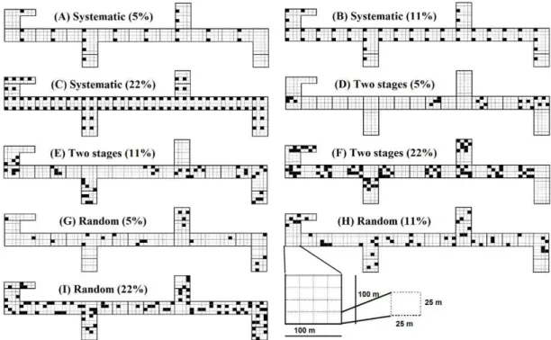
The forest remnant area was segmented into a mesh composed of 400 units of 25 m × 25 m, used for composing the samples for simulating processes and sampling intensities. Thus, three intensities were defined for the simulations to standardize the number of units sampled. In the first, a number of 20 sample units was established expressing 5% (1.25 ha) of the reference area (25 ha) (Figure 1A, D and G); the second included the measurement of 44 sample units, representing 11% of the population (2.75 ha) (Figure 1B, E, H); while the third considered 88 units, corresponding to 22% of the potential units (5.5 ha) (Figure 1C, F, I).
The processes were simulated for systematic sampling, two-stage sampling, and simple random sampling. In the systematic sampling, the sample units were selected in the stages between the lines (k1) and between units of the line (k2): a sample intensity of 5% was defined as the range k1 of 75 m and k2 of 200 m (Figure 1A); an intensity of 11% presented a k1 of 75 m and k2 of 100 m (Figure 1B), while a k1 of
75 m and k2 of 50 m were used for the intensity of
22% (Figure 1C). The interval between lines (k2) was
greater than the interval between lines (k1)due to the rectangular shape of the fragment,
The reference area was divided into 25 primary units (N) of one hectare each (100 m × 100 m) and subdivided into 16 secondary units (M) of 25 m × 25 m for the structural organization of the two-stage sampling. For the sampling intensity of 5%, five primary units (n) and later four secondary units (m) were randomized (Figure 1D). For the intensities of 11 and 22%, each primary unit consisted of 16 secondary units (M), of which four (Figure 1E) and eight units (m), respectively, were randomly selected from each selected primary unit (Figure 1F).
The method of selection without replacement was chosen for the simple random sampling, in which all possible combinations of potential sample units of the population had equal opportunity to participate in the sample, and 20, 44 and 88 sample units were selected for the intensities of 5% (Figure 1G), 11% (Figure 1H) and 22% (Figure 1I), respectively.
The Grubbs (1969) test was applied to the maximum values and then compared with the critical values at a
5% level of significance for analysis of the outliers. After their analysis, the descriptive statistics were calculated. Additionally, the normality of the data was verified by the Kolmogorov-Smirnov test (KS) for the probability of 95%. Next, the estimators of the sampling processes were calculated according to Péllico & Brena (1997), with the accuracy evaluated by the absolute (Ea) and relative (Er) errors and confidence interval (CI) at a 95% probability level.
2.4. Geostatistical modeling
The geostatistical analysis was applied for the spatial dependence model through semivariance (Equation 1), considering the geographical position of the sample units in the field, the subsequent computation of distances (h), and the numerical differences of the variable (Z) in the mesh of points (Isaaks & Srivastava, 1989). The semivariances were determined in four directions in the spatial plane: 0°, 45°, 90°, and 135°, and matrix of the mean half-variances between the equivalent distances was obtained and the possible anisotropic phenomena were verified (Yamamoto & Landim, 2013).
( ) N(h) ( ) ( ) 2
i i
i=1
1
h = { Z x - Z x +h } 2N(h)
γ
∑
(1)where: γ(h) = semivariance of the Z(xi) variable;
h = distance; and N(h) = number of pairs of Z(xi) and Z(xi+h) points measured, separated by a distance of h.
The spherical, exponential and Gaussian models were used to describe the spatial dependence structure
using the GS+ program (Robertson, 2008). For their
adjustment, the theoretical semivariogram structure was defined according to Yamamoto & Landim (2013) as C0 = nugget effect (the value of the semivariance for the zero distance, which represents the random variation component); C = contribution (structural variance);
C0 + C = threshold (the value of the semivariance in
which the curve stabilizes at a constant value); and A = range (distance from origin to the point at which the plateau reaches stable values).
The adjustment of the theoretical semivariograms was carried out by the Weighted Least Squares Method, with the evaluation and selection of the models performed based on the minimization of the weighted sum of squared deviations (WSSD), the highest coefficient
of determination (R2) and on cross-validation (R2)
(Isaaks & Srivastava, 1989), which considers the
linear, angular and determination coefficients of the cross-validation (R2
vc) and the standard error estimate (Syx%). They were staggered as a way to standardize the comparison between semivariograms according to the recommendation of Vieira et al. (1997).
The classification of Cambardella et al. (1994) was used to analyze the degree of spatial dependence (DD), in which semivariograms with a nugget effect less or equal to 25% of the plateau were considered as a strong DD; between 25 and 75% DD as moderate; and greater than 75% DD as weak. Subsequently, the interpolation was performed by ordinary point kriging (Equation 2), which consists of a non-skewed linear estimator with minimal variance for interpolation in non-sampled positions (Isaaks & Srivastava, 1989), in which the weights (λi) were determined by the Lagrange
multiplier technique (Webster & Oliver, 2007). Also,
the thematic maps were made using the GS+ program
(Robertson, 2008), considering the classes with absolute intervals of the basal area.
( ) n ( ) *
KO 0 i i
i=1
Z x =
∑
λ Z x (2)
where: * ( )
KO 0
Z x = ordinary kriging estimator; λi = weight;
i
Z(x ) = experimental data; and n = number of sample units.
The comparison of the mean basal area with the value observed in the census was made using the determination of the real error (Ereal%) as proposed by Augustynczik et al. (2013) to verify the consistency of the estimates through the simulated traditional samplings and the geostatistical interpolator (Equation 3). Thus, the aim of this study was to evaluate the quality of the geostatistical interpolator in estimating the basal area for native forests.
( ) real
(VE-VR)
E % = x100
VR (3)
where: VE = estimated value of the basal area by the sampling process and the geostatistical interpolator; and VR = real value of the basal area resulting from the census.
3. RESULTS AND DISCUSSION
3.1. Traditional estimators of sampling
processes
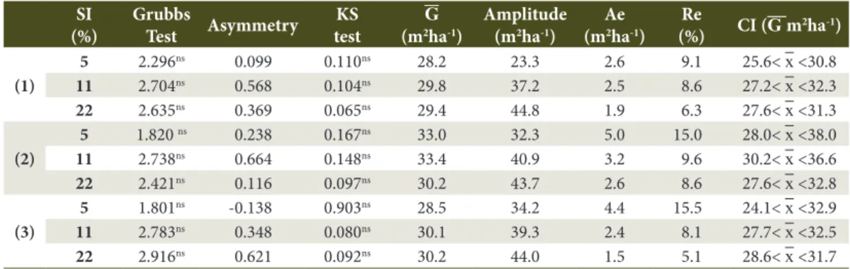
No outliers for the basal area variable were observed according to the Grubbs test, leading to a non-rejection of the null hypothesis (Table 1). The asymmetry values that express the tail extension of the distribution, ranged from -0.138 to 0.664, corroborating with the normal distribution at the 5% probability level by the Kolmogorov-Smirnov test (Table 1).
When analyzing the amplitude of the basal area, its direct relation with the sample intensity was noticed, which increased as the sample intensities intensified. This behavior is possibly justified by the diversity found in multi-native forests (Lima & Leão, 2013), whose remainder in the present study showed 117 species belonging to 44 botanical families, equivalent to 567 trees.ha-1, and not being sufficiently sampled at lower intensities.
For the estimation of the basal area, the lowest absolute (Ae) and relative (Re) errors for the intensity of 5% were found for the systematic sampling process, while the random sampling resulted in the best estimates for the intensities of 11 and 22% (Table 1), along with a tendency of smaller errors for greater intensities regardless of the sampling process tested, as observed in native forests studied by Cavalcanti et al. (2009) and Ubialli et al. (2009).
3.2. Geostatistical modeling
The presence of spatial dependence in all processes and sample intensities used to estimate the basal area was verified (Table 2). In general, a moderate to strong degree (of spatial dependence) was observed for the geostatistical adjustments, similar for each sample intensity regardless of the sampling process used, resulting in the possibility of generating maps regardless of the sample intensity used,corroborating with Kravchenko (2003).
The highest coefficients of determination (R2) and the lowest weighted sum of squared deviations (WSSD) were recorded for the sample intensity of 11% (Table 2) for all processes, in which the systematic sampling resulted in the best geostatistical adjustments, with R2 of 0.952 to 0.989 and WSSD of 0.001 to 0.007. On the other hand, the lowest R2 and the highest WSSD values were observed for the two-stage and the random processes at the intensity of 5%.
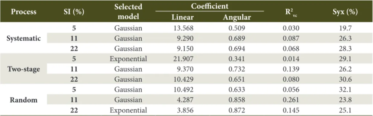
Overall, the Gaussian model stood out as the best for the semivariogram adjustments; it obtained
the lowest WSSD and the highest R2, except for the
two-stage and the random model at the intensities of 5 and 22%, respectively, in which the Exponential model was chosen in the cross-validation (Table 3).
The adjustments selected for the spatial modeling of the basal area in different sample intensities and processes resulted in linear coefficients of 3.856 to 21.907; angular coefficients between 0.341 and 0.872; cross-validation coefficients (R2
vc) of 0.030 to 0.145;
Table 1. Estimates of basal area using systematic sampling (1), two-stage sampling (2) and random simple sampling (3) in a Mixed Ombrophilous Forest remnant.
SI (%)
Grubbs
Test Asymmetry
KS test
G
(m2ha-1)
Amplitude (m2ha-1)
Ae (m2ha-1)
Re
(%) CI (G m2ha-1)
(1)
5 2.296ns 0.099 0.110ns 28.2 23.3 2.6 9.1 25.6< x <30.8 11 2.704ns 0.568 0.104ns 29.8 37.2 2.5 8.6 27.2< x <32.3 22 2.635ns 0.369 0.065ns 29.4 44.8 1.9 6.3 27.6< x <31.3
(2)
5 1.820 ns 0.238 0.167ns 33.0 32.3 5.0 15.0 28.0< x <38.0 11 2.738ns 0.664 0.148ns 33.4 40.9 3.2 9.6 30.2< x <36.6 22 2.421ns 0.116 0.097ns 30.2 43.7 2.6 8.6 27.6< x <32.8
(3)
5 1.801ns -0.138 0.903ns 28.5 34.2 4.4 15.5 24.1< x <32.9 11 2.783ns 0.348 0.080ns 30.1 39.3 2.4 8.1 27.7< x <32.5 22 2.916ns 0.621 0.092ns 30.2 44.0 1.5 5.1 28.6< x <31.7
Table 2. Parameters of the semivariograms adjusted for the basal area in the sample intensities and processes in a Mixed Ombrophilous Forest remnant.
Process SI (%) Model C0 C A (m) DD (%) R2 WSSD
Systematic 5
Spherical 0.64 29.72 152.6 2.1 0.827 0.0041 Exponential 0.64 29.88 158.9 2.1 0.742 0.0049 Gaussian 11.00 19.52 155.6 36.0 0.824 0.0040
11
Spherical 20.98 45.73 189.6 31.5 0.982 0.0002 Exponential 1.37 68.33 187.3 2.0 0.952 0.0007 Gaussian 34.10 33.10 182.6 50.7 0.989 0.0001
22
Spherical 31.64 42.28 135.6 42.8 0.887 0.0019 Exponential 7.50 68.04 130.1 9.9 0.892 0.0018 Gaussian 40.28 33.83 127.0 54.4 0.891 0.0018
Two-stage 5
Spherical 1.86 111.08 126.3 1.6 0.540 0.0170 Exponential 31.03 74.72 118.2 29.3 0.682 0.0050 Gaussian 54.85 51.81 122.3 51.4 0.663 0.0063
11
Spherical 27.91 65.83 178.6 29.8 0.847 0.0067 Exponential 6.35 88.88 182.6 6.7 0.808 0.0079 Gaussian 43.13 51.97 175.3 45.4 0.871 0.0053
22
Spherical 46.79 53.18 183.6 46.8 0.707 0.0066 Exponential 31.95 70.77 198.6 31.1 0.662 0.0074 Gaussian 57.21 43.67 169.3 56.7 0.723 0.0063
Random
5
Spherical 16.85 68.64 201.6 19.7 0.746 0.0191 Exponential 1.87 86.11 206.3 2.1 0.739 0.0179 Gaussian 31.37 57.87 206.3 35.2 0.795 0.0156
11
Spherical 10.52 50.28 189.6 17.3 0.915 0.0026 Exponential 1.43 59.82 188.3 2.3 0.908 0.0034 Gaussian 21.99 39.95 185.3 35.5 0.953 0.0013
22
Spherical 64.30 28.30 180.9 69.4 0.673 0.0041 Exponential 49.30 44.18 165.2 52.7 0.719 0.0039 Gaussian 68.70 23.79 151.1 74.3 0.663 0.0042
SI = Sample intensity; Co = Nugget effect; C = Structural variance; A = range; DD = Degree of spatial dependence; R
2 = Coefficient of determination; and WSSD = weighted sum of squared deviations.
Table 3. Cross-validation of the geostatistical adjustments selected for the sample intensities and processes in a Mixed Ombrophilous Forest remnant.
Process SI (%) Selected
model
Coefficient
R2
vc Syx (%)
Linear Angular
Systematic
5 Gaussian 13.568 0.509 0.030 19.7
11 Gaussian 9.290 0.689 0.087 26.3
22 Gaussian 9.150 0.694 0.068 28.3
Two-stage
5 Exponential 21.907 0.341 0.014 29.1
11 Gaussian 9.370 0.732 0.139 26.2
22 Gaussian 10.429 0.651 0.080 30.6
Random
5 Gaussian 10.492 0.633 0.056 32.1
11 Gaussian 4.287 0.858 0.261 23.8
22 Exponential 3.856 0.872 0.145 25.1
SI = Sample intensity; R2
vc = Cross-validation coefficient of determination; and Syx% = Standard error of estimate in percentage.
and standard error estimates (Syx%) from 19.7 to 30.6% (Table 3). It was observed that the linear and angular coefficients were distant from the ideal theoretical
values, in addition to acceptable low R2
vc and Syx% considering the heterogeneity characteristics of the tropical forest structure.
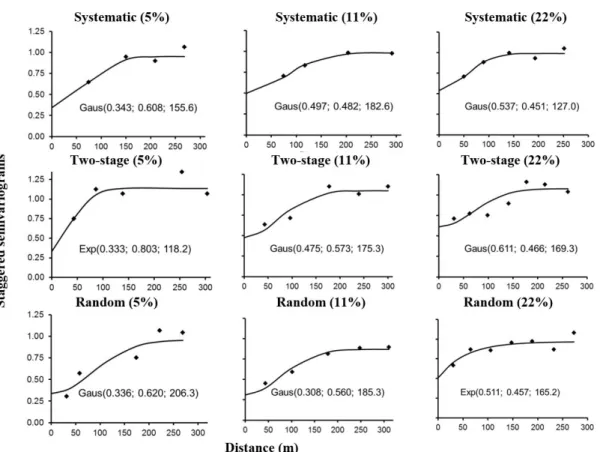
the intensities of the two-stage process and for the random sampling at the intensity of 5% of the sampled area. In addition, isotropic behavior was admitted due to the similarity of directional semivariograms in the spatial plane.
Estimates of the nugget effect (Co) increased among the sampling processes to estimate the basal area, while the contribution (C) decreased with the increase in sample intensity (Figure 2). Thus, there was a tendency to modify the spatial structure detected by the geostatistical analyzes. According to Mello et al. (2006), it is common to observe lower nugget effect values at higher intensities in the executed inventories with a low number of sample units.
Figure 3 shows that the increase in sample intensity provided greater detail of the kriging information in basal area classes, except for the random process. This detailing in the variation patterns of the maps becomes increasingly degraded with the increase in the distance between the sample units and the decrease in the sampling intensity (Souza et al., 2014).
Different spatial patterns were observed among the intensities of the systematic sampling process, with a predominance of class IV of the basal area at intervals ranging from 26.0 to 32.2 m2 ha-1; followed by class III at the intensity of 5%; and by class V at the intensities of 11 and 22% (Figure 3A up to 3C). For the two-stage sampling process (Figure 3D up to 3F), the 5% intensity resulted in three basal area classes and in greater homogeneity, with values between 26.0 and 44.6 m2 ha-1, as the intensities of 11 and 22% were represented by the lower classes. Again, a predominance of the class IV basal area was observed.
When comparing the estimates for the random process (Figure 3G up to 3I), the greatest variability was found for sample intensity of 11% with the definition of six classes of basal area, while five and four classes were defined for the intensities of 5 and 22%, respectively. The most extensive stratum was represented by class IV, followed by class III at the 5% intensity, and by class V at the intensities of 11 and 22%.
3.3. Comparison between traditional and the
geostatistical interpolator estimators
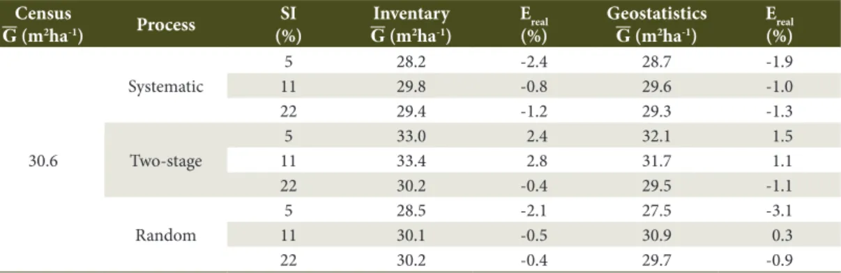
The systematic process tended to present a lower mean basal area than in the random sampling, with errors of -0.5 and 0.3% for the inventory and the
geostatistical interpolator, respectively, while the two-stage process resulted in overestimations of 1.1 and 2.8% in relation to the census (Table 4). In general, the estimates resulted in values with mean difference lower than 1%, except for the two-stage sampling at the intensity of 11%.
Figure 3. Thematic maps of the basal area for the sample intensities and processes in a Mixed Ombrophilous Forest remnant.
Table 4. Mean basal area observed and estimated by the sampling processes and the geostatistical interpolator in a Mixed Ombrophilous Forest remnant.
Census
G (m2ha-1) Process
SI (%)
Inventary
G (m2ha-1)
Ereal (%)
Geostatistics
G (m2ha-1)
Ereal (%)
30.6
Systematic
5 28.2 -2.4 28.7 -1.9
11 29.8 -0.8 29.6 -1.0
22 29.4 -1.2 29.3 -1.3
Two-stage
5 33.0 2.4 32.1 1.5
11 33.4 2.8 31.7 1.1
22 30.2 -0.4 29.5 -1.1
Random
5 28.5 -2.1 27.5 -3.1
11 30.1 -0.5 30.9 0.3
22 30.2 -0.4 29.7 -0.9
Despite the quality of the estimates by the geostatistical interpolator, the major underestimates and overestimations of the basal area occurred in the random and two-stage processes at the 5% intensity, respectively. Scolforo et al. (2016) evaluated the best spatial technique for mapping the above-ground carbon stock of tree vegetation and identified that no interpolator is robust enough to capture the pattern for extreme values. The largest errors in the census were observed for sample the 5% intensity (Table 4), as reported by Augustynczik et al. (2013).
It was observed that all the sampling processes presented adequate estimates for the basal area, with an advantage for the geostatistical modeling in the systematic and the two-stage sampling processes for the intensity of 5%. The geostatistical interpolator resulted in a smaller error for the random process at 11% intensity, while the traditional sampling estimator presented the best estimates for the intensity of 22% in the two-stage and random processes.
In studies with the species Quercus suber in Spain, Montes et al. (2005) observed that when the basal area presented spatial continuity, random sampling has a greater standard error than systematic sampling. Contrary results have been observed by Lundgren et al. (2015) in Eucalyptus stands in the semiarid of Pernambuco, where random sampling showed the best results for estimating the individual eucalyptus volume performed by the geostatistical analysis. Thus, it is observed that spatial continuity is influenced by the different forest physiognomies, in addition to the various methods and sampling intensities.
4. CONCLUSION
Traditional forest inventory estimators and the geostatistical interpolator present adequate results when compared to those obtained by forest census, in which the average difference is less than 1%. Thus, incorporating the spatial component in forest inventory processing has the ability to improve the accuracy of basal area estimates of native forests, while the increase in sample intensity for systematic and two-stage sampling allow a greater level of detail of the basal area spatial behavior for composing thematic maps using geostatistical modeling.
SUBMISSION STATUS
Received: 13 aug., 2017 Accepted: 5 dec., 2017
CORRESPONDENCE TO
Marcelo Roveda
Departamento de Engenharia Florestal, Universidade Federal do Paraná – UFPR,
Avenida Pref. Lothário Meissner, CEP 80060-000, Curitiba, PR, Brasil
e-mail: [email protected]
REFERENCES
Akhavan R, Kia-Daliri H, Etemad V. Geostatistically estimation and mapping of forest stock in a natural unmanaged forest in the Caspian region of Iran. Caspian Journal of Environmental Sciences 2015; 13(1): 61-76.
Alvares CA, Stape JL, Sentelhas PC, Gonçalves JLM, Sparovek G. Koppen’s climate classification map for Brazil. Meteorologische Zeitschrift 2013; 22(6): 711-728. http:// dx.doi.org/10.1127/0941-2948/2013/0507.
Augustynczik ALD, Machado AS, Figueiredo A Fo, Péllico S No. Avaliação do tamanho de parcelas e de intensidade de amostragem em inventários florestais. Scientia Forestalis 2013; 41(99): 361-368.
Brandelero C, Giotto E, Watzlavick LF, Pereira RS, Andreis S. Tecnologia móvel utilizada no inventário florestal. Floresta 2008; 38(4): 727-734. http://dx.doi.org/10.5380/ rf.v38i4.13168.
Cambardella CA, Moorman TB, Parkin TB, Karlen DL, Novak JM, Turco RF et al. Field-scale variability of soil properties in central Iowa soils. Soil Science Society of America Journal 1994; 58(5): 1501-1511. http://dx.doi. org/10.2136/sssaj1994.03615995005800050033x.
Campos JCC, Leite HG. Mensuração florestal: perguntas e respostas. 4. ed. Viçosa: UFV; 2013.
Cavalcanti FJB, Machado SAM, Hosokawa RT. Tamanho de unidade de amostra e intensidade amostral para espécies comerciais da Amazônia. Floresta 2009; 39(1): 207-214. http://dx.doi.org/10.5380/rf.v39i1.13740.
Corte APD, Sanquetta CR, Figueiredo A Fo, Pereira TP, Behling A. Desempenho de métodos e processos de amostragem para avaliação de diversidade em Floresta Ombrófila Mista. Floresta 2013; 43(4): 579-582. http:// dx.doi.org/10.5380/rf.v43i4.30526.
Freitas WK, Magalhães LMS. Métodos e parâmetros para estudo da vegetação com ênfase no estrato arbóreo. Floresta e Ambiente 2012; 19(4): 520-540. http://dx.doi. org/10.4322/floram.2012.054.
Grubbs FE. Procedures for detecting outlying observations in samples. Technometrics 1969; 11(1): 1-21. http://dx.doi. org/10.1080/00401706.1969.10490657.
Higuchi N. Amostragem sistemática versus amostragem aleatória em floresta tropical úmida de terra firme na região de Manaus. Acta Amazonica 1987; 16/17(1): 393-400.
Isaaks EH, Srivastava RM. An introduction to applied geostatistics. New York: Oxford University Press; 1989.
Kravchenko AN. Influence of spatial structure on accuracy of interpolation methods. Soil Science Society of America Journal 2003; 67(5): 1564-1571. http://dx.doi.org/10.2136/ sssaj2003.1564.
Lima JPC, Leão JRA. Dinâmica de crescimento e distribuição diamétrica de fragmentos de florestas nativa e plantada na Amazônia Sul Ocidental. Floresta e Ambiente 2013; 20(1): 70-79. http://dx.doi.org/10.4322/floram.2012.065.
Lundgren WJC, Silva JAS, Ferreira RLC. Estimação de volume de madeira de eucalipto por cokrigagem, krigagem e regressão. Cerne 2015; 21(2): 243-250. http://dx.doi.or g/10.1590/01047760201521021532.
Machado AS, Figueiredo A Fo. Dendrometria. 3. ed. Guarapuava: Unicentro; 2006.
Mello JM, Oliveira MS, Batista JLF, Justiniano PR Jr, Kanegae H Jr. Uso do estimador geoestatístico para predição volumétrica por talhão. Floresta 2006; 36(2): 251-260. http://dx.doi.org/10.5380/rf.v36i2.6454.
Montes F, Hernandez MJ, Canellas IA. geostatistical approach to cork production sampling in Quercus suber forests. Canadian Journal of Forest Research 2005; 35(12): 2787-2796. http://dx.doi.org/10.1139/x05-197.
Péllico S No, Brena D. Inventário florestal. Curitiba: Universidade Federal do Paraná; 1997.
Pereira JC, Dias PAS, Mergulhão RC, Thiersch CR, Faria LC. Modelo de crescimento e produção de Clutter adicionado de uma variável latente para predição do volume
em um plantio de Eucalyptus urograndis com variáveis correlacionadas espacialmente. Scientia Forestalis 2016; 44(110): 1-12. http://dx.doi.org/10.18671/scifor.v44n110.12.
Robertson GP. GS+: geostatistics for the environmental sciences. Michigan: Plainwell; 2008.
Scolforo HF, Scolforo JRS, Mello JM, Mello CR, Morais VA. Spatial interpolators for improving the mapping of carbon stock of the arboreal vegetation in Brazilian biomes of Atlantic forest and Savanna. Forest Ecology and Management 2016; 376: 24-35. http://dx.doi.org/10.1016/j. foreco.2016.05.047.
Scolforo JRS, Mello JM. Inventário florestal. 1. ed. Lavras: UFLA/FAEPE; 2006.
Souza AL, Soares CPB. Florestas nativas: estrutura, dinâmica e manejo. Viçosa: Editora UFV; 2013.
Souza ZM, Souza GS, Marques J Jr, Pereira GT. Número de amostras na análise geoestatística e na krigagem de mapas de atributos do solo. Ciência Rural 2014; 44(2): 261-268. http://dx.doi.org/10.1590/S0103-84782014000200011.
Ubialli JA, Figueiredo A Fo, Machado AS, Arce JE. Comparação de métodos e processos de amostragem para estimar a área basal para grupos de espécies em uma floresta ocotonal da região norte matogrossense. Acta Amazonica 2009; 39(2): 305-314. http://dx.doi. org/10.1590/S0044-59672009000200009.
Vieira SR. Uso de geoestatística em estudos de variabilidade espacial de propriedades do solo. In: Novais RF, Alvarez VH, Schaefer CEGR, editors. Tópicos em ciência do solo. Viçosa: Sociedade Brasileira de Ciência do Solo; 2000.
Vieira SR, Tillotson PM, Biggar JW, Nielsen DR. The Scaling of semivariograms and the kriging estimation of field-measured properties. Revista Brasileira de Ciência do Solo 1997; 21(4): 525-533. http://dx.doi.org/10.1590/ S0100-06831997000400001.
Webster R, Oliver MA. Geostatistics for environmental scientists. 2. ed. Chichester: John Wiley & Sons; 2007. http://dx.doi.org/10.1002/9780470517277.