Macroeconomics determinants of loss given default

(1)

Macroeconomic Determinants of Loss Given Default

Supervisor

João Afonso Bastos

Candidate

Henrique Sousa de Azevedo

Master of Science in Finance Final Work Dissertation

(2)

Macroeconomic Determinants of Loss Given Default

Supervisor: João Afonso Bastos (ISEG - UL) Candidate: José Henrique Sousa de Azevedo

(3)

Declaration of Originality

I, Henrique Sousa de Azevedo, hereby declare that this dissertation is my own work and has not been submitted in any form for another degree or diploma at any university or other institute of tertiary education. Information derived from the published and unpublished work of others has been acknowledged in the text and a list of references is given in the References section.

(4)

Acknowledgements

I would like to gratefully acknowledge and sincerely thank my supervisor, Professor João Bastos, for his guidance and patience throughout the writing of this dissertation. Without his suggestions and help, it would never get written.

Also, my deepest appreciation to the late Professor Carlos Mendonça e Moura (Faculty of Engineering, University of Porto), for his encouragement and for sharing with me his knowledge of statistics.

Lastly, to the Lisbon School of Economics and Management (ISEG), University of Lisbon, for granting me access to its databases and library.

(5)

Abstract

This dissertation models Moody's Ultimate Recovery Database to show that general macroeconomic conditions influence loss given default and that loans' recovery rates are less susceptible to macroeconomic conditions than bonds'. Available data was studied with Ordinary Least Squares regressions. Alternative methodologies are also discussed.

(6)

1. Introduction

Renowned investor and Berkshire Hathaway's Chairman, Warren Buffett once said, "Risk comes from not knowing what you're doing". This assertion is particularly relevant given recent occurrences in the financial markets and the global economy. The global financial crisis has made risk analysis a key issue for financial institutions and governments alike, justifying the ever-expanding strand of practitioner literature and academic papers on the subject. This dissertation aims to make a small contribution to that study by providing research into one of the three components of credit risk: loss given default.

Credit risk - the risk stemming from a borrower (the obligor) failing to meet his contractual obligations towards creditors, namely, repaying loans and other credit instruments - is assessed resorting to three different parameters: (i) probability of default (PD); (ii) exposure at default (EAD) and (iii) loss given default (LGD).

PD is an estimate, in percentage terms, of the likelihood that the obligor (the debtor) will be unable to meet its debt obligation over a certain time horizon. According to Basel II1_{criteria, a default events on an obligation occurs}

if: (a) the obligor is unlikely to be able to repay its debt without giving up any pledged collateral, or (b) the obligor has passed more than 90 days without paying a material credit obligation.

1_{Basel II is the second of the Basel Accords, which are recommendations on}

banking laws and regulations issued by the Basel Committee on Banking Supervision.

(8)

EAD expresses the amount the creditor is likely to lose in the event of an obligor defaulting and it is measured in currency. According to the Bank of International Settlements (BIS), EAD must not be lower than the book value of balance sheet receivables and has to be calculated without considering provisions. Under Basel II guidelines, banks meeting certain minimum conditions are allowed to adopt an Internal Ratings-Based Approach (IRB)2_{, i.e., their own}

estimated risk parameters, when calculating EAD.

LGD is the loss incurred by a financial institution when an obligor defaults on a loan, given as the fraction of exposure at default (EAD) unpaid after some period of time. LGD, which refers to bonds as well as loans, is an essential element in calculating regulatory capital requirements under the Basel II framework. It is common practice to model LGD using recovery rates, i.e., the proportion of a defaulted debt instrument (principal and accrued interest) that can be recovered, expressed in percentage terms. LGD is therefore calculated as 1 - recovery rate.

We have attempted to ascertain whether general market conditions influence recovery rates, commonly known as recoveries, by tracking some macroeconomic variables over a period of time and applying statistical procedures to the data compiled.

2_{Basel II only allows banks meeting certain transparency criteria to adopt an IRB}

(9)

1.1 Literature Review

Understanding LGD is paramount to better understanding credit risk, but this is a subject whose study has been fraught with difficulties, namely: (i) the lack of recovery observations, as many financial institutions do not possess sufficiently complete datasets; (ii) the complexity of the recovery process, as access to collateral in case of default is often problematic; and (iii) the lack of empirical evidence to determine predictive factors.

The first big question when approaching the subject of LGD is well summarized in Frye (2005): when forecasting the losses stemming from credit default, it has to be assumed LGD varies independently or that, on the contrary, it is sensitive to economic downturns, and thus sensitive to macroeconomic factors. Proponents of LGD independence argued that no convincing evidence could be summoned that systematic LGD risk is real. Others, on the other hand, counter that an obligor's assets are sensitive to systematic risk, both before and after a default event. The conclusion is, therefore, that, in a downturn, recovery should be lower and LGD greater. Perhaps the financial crisis of 2007-2008 has made this debate redundant, giving strength to the assumption that macroeconomic conditions are, indeed, relevant to the study of LGD, as this dissertation's Descriptive Analysis section further ahead shows. Frye (2005) is therefore pivotal, warning that LGD's sensitivity works against managers of risky assets, because it increases loss in high default periods.

Historically, early authors on the subject of recovery rates and LGD tended to focus on bond markets, but lately loans have also been the object of

(10)

several studies. Furthermore, several authors have proposed different paths to modeling LGD, some of which shall be discussed hereon.

Jankowitsch, Nagler and Subrahmanyam (2014) examines recovery rates of defaulted bonds in the US corporate bond market over an approximately 8-year period of time (2002 to 2010), using a significant array of variables. Among these, were the following macroeconomic indicators: (i) the market-wide default rate, (ii) the industry-specific default rate, (iii) the Federal Funds rate and (iv) the slope of term-structure of interest rates. Importantly, it concludes macroeconomic variables are clearly linked to recovery rates.

Bruche and González-Aguado (2010) presents a predictive model to characterize systematic credit risk, using a dataset of more than 2000 defaulted bonds of US firms from 1974 to 2005. It attempts to empirically illustrate the time-series behavior of default probabilities and recovery rates distributions. In the model, both depend on an unobserved two-state Markov chain; interpreted as a "credit cycle", i.e., the estimated states correspond to periods of economic downturn, in which default probabilities are high and recoveries low, and to periods of upturn, in which the reserve is true. Controversially, it suggests that default rates and recovery rates are more tightly related to each other than to macroeconomic variables and that credit downturns seem to be only imperfectly aligned with recessions (starting before recessions and lasting longer).

Acharya, Bharath and Srinivasan (2007) also attempts to empirically document the determinants of recovery rates, using a dataset on US defaulted firms data (bonds, loans and other debt instruments) for 1982-1999. A univariate analysis is performed on an additive model, followed by a multivariate

(11)

analysis (a similar procedure to the one followed in this dissertation). It finds industry conditions at the time of default are important determinants of recoveries, particularly in periods of distress, arguing the case for the importance of considering industry factors when modeling credit risk. If Acharya, Bharath and Srinivasan (2007)'s comments on industry conditions are accepted, it may be argued that wider factors and macroeconomic variables are not particularly to the study LGD, meriting further discussion.

Literature specifically investigating recovery rates of loans usually falls under one of two categories: (i) empirical studies analyzing the level of the recovery rates, which variables might influence recoveries and predictive statistical models; (ii) studies criticizing the assumption of credit risk models concerning recovery rates, mostly questioning the assumption that PD and recoveries are independent variables.

As previously mentioned and also discussed in Dermine and Neto de Carvalho (2006)'s study of Banco Comercial Português's loan losses, existing empirical literature on credit risk has focused more on bonds rather than loans, since few data on bank loan losses - essentially, private instruments - are publicly available. It is also observed that these studies tend to focus on the US corporate bond market. The authors estimated LGD on a sample comprising 374 corporate loans from 1995 to 2000, concluding the average recovery (71%) is similar to that obtained in US studies. Applying a multivariate approach to the dataset, it was found loan losses given default were bi-modal (either null or nearly 100%) and that certain variables (size of the loan, collateral, industry sector, year dummies and age of the firm) are relevant to the study of LGD. Also,

(12)

it was concluded the costs incurred by BCP in recovery were in the same order as those obtained in studies on US bankruptcies.

More recently, loan losses have also been the scope of some studies, such as those undertaken in Khieu, Mullineaux and Yi (2012) and Bellotti and Crook (2012).

Khieu, Mullineaux and Yi (2012) stresses the importance of understanding the factors that influence bank loans recoveries following default and of treating bonds and loans separately. This study based itself on a similar database to the one used in this dissertation (a previous version of Moody's Ultimate Recovery Database - URD, comprising data for 1987-2007), used to estimate a model for bank loan recoveries. This model incorporates variables reflecting loan and borrower characteristics, industry and macroeconomic conditions, as well as several process recovery variables. It found that loan characteristics are, in general, more significant as determinants of recovery rates than borrower characteristics prior to default. Industry conditions were also found to be relevant. Importantly, macroeconomic conditions were also judged relevant, but the probability of default at the time of loan origination was found to be unrelated to ultimate recoveries. Finally, it shows that firm leverage before default negatively affects ultimate recoveries and secured loans have higher recoveries. Loans to borrowers with prior defaults were found to yield higher recoveries than first-time defaults.

Bellotti and Crook (2012) also observes - as, indeed, does all literature reviewed - that LGD is not usually modeled directly; recovery rates are used instead. The authors' case study is the UK's credit card market, used to develop

(13)

and test several LGD models, including Tobit, a decision tree model, a Beta and a fractional logit transformation. It is concluded ordinary least squares (OLS) with macroeconomic variables fares best for forecasting LGD3_{at account and portfolio}

levels and that bank interest rates and the unemployment level significantly affect LGD. It also confirms Dermine and Neto de Carvalho's (2006) conclusion that loan size is a significant explanatory variable for recoveries, adding that the obligor's age has a negative effect on recoveries (thus, a positive relation to LGD).

Acharya et. al. (2007) also applies OLS modeling; in this case to US defaulted firms data (bonds, loans and other debt instruments) for 1982-1999, concluding - as previously quoted studies did - that recovery rates are heavily influenced by whether the industry of the defaulted firm is in distress or not. As common sense would have it, creditors recover less if the industry is in distress and if non-defaulted firms are illiquid. Evidence suggests that an instrument's recovery rate is influenced by how its peers perform, i.e., in times of distress, a decrease in recoveries is caused by the expected downward revision of a firm's worth, but also by the financial constraints its peers face. It is likely this is a sector-wide effect, as certain external effects may affect all firms within a certain sector or because of a certain level of interconnectedness amongst same-sector companies.

Caselli et. al. (2008) follows a similar approach assessing the sensitivity of LGD to systematic risk. This paper, which has a subject similar to this

3_{Bellotti and Crook (2012) claim it is difficult to explain why OLS is the best}

approach for modeling LGD, but that - having tried different combinations of variables, as well as various transformation on the dependent variable - this conclusion has been reached consistently.

(14)

dissertation's, verifies the existence of a relation between households' and small-and-medium enterprises' LGD and macroeconomic conditions in the Italian loan market. It stresses the importance of distinguishing between household losses and corporate losses, arguing the former are susceptible to macroeconomic variables such as the default-to-loan ratio, the unemployment rate and household consumption, whilst the latter are more sensitive to changes in the total number of employed people and the GDP growth rate.

Furthermore, OLS modeling is also adopted in Grunert and Weber's (2009) paper on bank loans' recovery rates, which finds that a high quota of collateral leads to higher recovery rates and suggests a negative relation between the obligor's creditworthiness and recovery rates.

Gupton & Stein (2005) follows an alternative path. This paper, in which a widely known LGD predictive model for bonds, loans and stocks is presented (LossCalc v2), starts out by transforming the raw data to create more powerful univariate factors, "mini models". Real modeling starts by determining the appropriate weights to combine the transformed variables and "mini models". The combination of the predictive factors is a linear weighed sum, derived using regression techniques without the intercept term. It thus takes the form of an additive model. Only subsequently are standard OLS multivariate regression techniques applied. Recoveries are normalized via a beta distribution.

It should be stressed that, despite the extensive use of OLS regressions in LGD modeling, more recent studies have proposed other approaches to modeling recovery rates. Besides generalized linear models (GLM), other, more sophisticated approaches, such as regression trees and neural networks (Bastos,

(15)

2010a; Bastos, 2010b; Qi and Zhao, 2011), have also recently been the object of discussion within the academic community.

Bastos (2010a) tests several alternative models on BCP's data, proposing the use on nonparametric regression trees when modeling bank loans' recoveries. Regression trees are nonparametric and nonlinear models that partition data into smaller sets using an algorithm. It is argued that tree models resemble "look-up" tables containing historical recovery averages. This study also discusses the use of fractional response regressions, an alternative to be considered when the dependent variable is bounded between 0 and 1. This makes implementing an OLS regression difficult, since OLS predicted values can never be guaranteed to lie in the unit interval.

Bastos (2014) uses data from Moody's URD to show how to implement a successful ensemble strategy for predicting recovery rates on defaulted debts. It labors on the assumption that a committee of experts' opinion is always more desirable than an individual opinion, thus providing gains in predictive power. It argues that a successful strategy should be based on a predictor that combines the opinion of an ensemble of structurally similar models estimated on perturbed versions of the original data. An ensemble of regression trees is shown to outperform the forecasts given by a single regression tree. The study finds that industry, collateral and instrument type dummy variables are not of the greatest relevance, importantly concluding that debt priority in the liability structure heavily contributes to the recovery rate.

Continuing to explore nonparametric mathematical models (besides regression trees), in Bastos (2010b) another alternative to model recoveries is

(16)

presented: artificial neural networks4_{. It is important to note that results}

obtained with neural networks have, however, shown some divergence to those attained by fractional regression models.

Qi and Zhao (2011) also addresses the modeling issue by comparing six modeling methods for LGD (parametric - OLS regression, fractional response regression, inverse Gaussian regression and inverse Gaussian regression with beta transformation; nonparametric - regression tree, neural network), using Moody's URD as sample. It is found nonparametric methods outperform parametric methods in terms of model fit and predictive accuracy. Of those - and both provided high predictive accuracy - the neural network was shown to be the most reliable method. Parametric methods, even if not as effective, also provided decent model fit, with the fractional response regression showing slightly better goodness-of-fit than the OLS regression. Interestingly, it also suggests a strong bi-modal distribution does not necessary equate to accurate LGD estimation, arguing it may only be of secondary importance in predicting LGD.

Loterman et. al. (2012) deepens this discussion, comparing a total of 24 techniques (both one-stage and two-stage models) on 6 different datasets, making it a truly large-scale study. Most models were found to have limited explaining power, with R2 _{in the 4% - 43% range. It also sustains than non-linear}

methods, in particular support vector machines5_{and neural networks, perform}

4_{Bastos (2010b) uses the same database as Bastos (2010a): 374 loans to small}

and medium enterprises granted by Banco Comercial Português (BCP).

5_{Support vector machines are models with associated learning algorithms that}

(17)

better than linear techniques and suggests the use of a two-stage setting, combining nonlinear methods with a linear component as a way to better study LGD.

2. Dataset description

2.1 The Database

Our data set consists of Moody's Ultimate Recovery Database (URD), which comprises data on 4630 bonds and loans from 957 issuers that defaulted between 1987 and 2010. These issuers are US nonfinancial corporations holding over $50 million in debt at the time of default.

Moody's follow Basel II guideline and adopt multiple approaches to recovery calculation, providing three separate methods for nominal and discounted recovery (settlement, trading price and liquidity) and indicating which is considered to be most appropriate. We follow Moody's suggestion and use whichever the rating agency favors. Moody's variables6_{include dummy}

variables for industry, collateral and instrument type, as well as the percentage of obligors' debt senior to the instrument (percentage above), the percentage of obligors' debt junior the instrument (percentage below) and the instrument rank within the obligor's liability structure.

the algorithm analyzes the training data, which it then uses to produce an inferred function, used for mapping new examples.

(18)

Moody's URD has been in several academic studies, among which Qi and Zhao (2011), Khieu, Mullineaux and Yi (2012) and Bastos (2014), making it a reference dataset for the study of recovery rates and LGD.

We added our own macroeconomic variables to Moody's URD, using monthly data whenever possible. If unavailable, we resorted to quarterly or yearly data. Our macroeconomic and financial variables are: (i) quarterly GDP changes, in USD, chained to 2009 US dollars, seasonally adjusted; (ii) monthly 10-year Treasury Constant Maturity Rate, not seasonally adjusted; (iii) the National Bureau of Economic Research (NBER) recession indicator (monthly data); (iv) total number of US corporate defaults (yearly data); (v) US corporate default rate (yearly data) and S&P 500 monthly total return changes.

The data for these variables are in the public domain and were obtained from the US Department of Commerce's Bureau of Economic Analysis, the Federal Reserve Bank of St. Louis, the National Bureau of Economic Research and Standard & Poor's.

We have also taken care to discriminate bonds from loans since, according to Khieu et. al. (2012), treating them together carries the implicit assumption that the same factors influence recovery rates in both markets in identical ways, thus ignoring different categories of financial instruments have different characteristics. Furthermore, Acharya, Bharath and Srinivasan (2007) and Varma and Cantor (2005) state that bank loans are more likely to be secured than bonds and that, on average, secured lenders recover more than unsecured creditors. Given also that bank loans are usually senior to bonds, it makes sense

(19)

to treat them separately, in order to better understand the relevance of macroeconomic factors to our models.

2.2 Descriptive Analysis

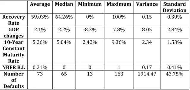
Inspecting Table 1, which displays some descriptive statistics of our dataset, it is observed the average recovery rate is nearly 60%; consequently, average LGD is just above 40%. This is substantiated by the median - a similar value - indicating low skewedness. The yearly number of default events varies considerably, but - more significantly - corporate default rates remain considerably low. A possible explanation for these corporate rates is that, ever since the financial crisis, companies have either been cutting back on debt or refinancing their debt at lower interest rates. Considering low interest rates, credit markets exhibiting higher liquidity than previously and some economic growth, this it is understandable.

Table 1 - Descriptive Statistics for Bonds and Loans

Average Median Minimum Maximum Variance Standard Deviation Recovery Rate 59.03% 64.26% 0% 100% 0.15 0.39% GDP changes 2.1% 2.2% -8.2% 7.8% 8.05 2.84% 10-Year Constant Maturity Rate 5.26% 5.04% 2.42% 9.36% 2.34 1.53% NBER R.I. 0.21% 0 0 1 0.17 0.41% Number of Defaults 73 65 13 163 1914.47 43.75%

(20)

Default

Rate 2.75% 2.92% 0.49% 5.71% 2.11 1.455%

S&P 500 0.61% 0.88% -16.79% 11.44% 21.62 4.655%

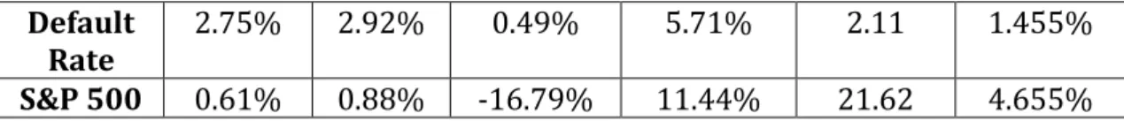
Comparing now Table 2 and Table 3, discriminating statistics for bonds and loans, respectively, some interesting conclusions may be drawn. Firstly, the recovery rate for loans is nearly double that of bonds (and the median, triple), substantiating Acharya, Bharath and Srinivasan (2007)'s and Varma and Cantor (2005)'s previously mentioned statement that bank loans are more likely to be secured than corporate bonds. Secondly, the default rate for both instruments is nearly the same, so are the number of defaults and S&P 500 return changes. This strengthens the aforementioned argument, possibly because most loans have some form of collateral. In the case of obligor default, collateral may be used to repay creditors.

Table 2 - Descriptive Statistics for Bonds

Average Median Minimum Maximum Variance Standard Deviation Recovery Rate 44.84% 36.28% 0% 100% 0.14 0.37% GDP changes 2.07% 2.2% -8.2% 7.8% 7.62 2.765 10-Year Constant Maturity Rate 5.38% 5.09% 2.42% 9.36% 2.53 1.59% NBER R.I. 0.21% 0 0 1 0.17 0.41% Number of Defaults 71 65 13 163 1847.57 42.98% Default Rate 2.73% 2.92% 0.49% 5.71% 2.03 1.42% S&P 500 0.65% 0.81% -16.79% 11.44% 21.11 4.6%

(21)

Table 3 - Descriptive Statistics for Loans

Average Median Minimum Maximum Variance Standard Deviation Recovery Rate 80.43% 100% 0% 100% 0.09 0.30% GDP changes 2.14% 2.2% -8.2% 7.8% 8.7 2.95% 10-Year Constant Maturity Rate 5.07% 4.91% 2.42% 9.36% 2 1.41% NBER R.I. 0.21% 0 0 1 0.16 0.41% Number of Defaults 75 65 13 163 2004.45 44.77% Default Rate 2.77% 2.47% 0.49% 5.71% 2.22 1.49% S&P 500 0.32% 0.97% -16.79% 11.44% 25.08 5.01%

3. Results

3.1 Model for the complete data set

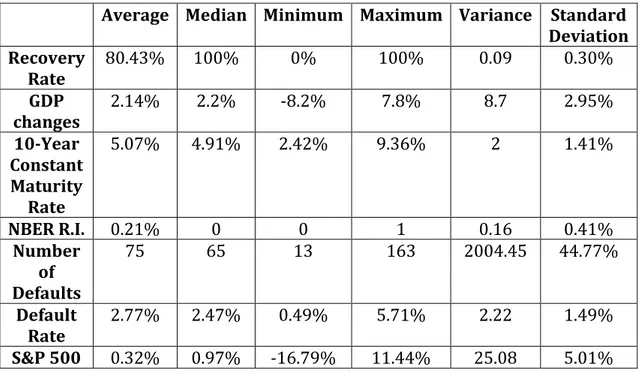
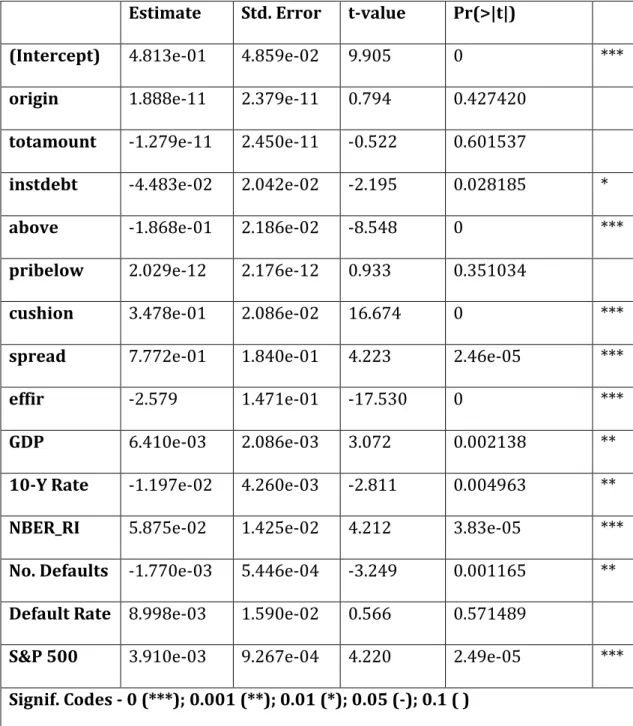
Table 4 shows the results of the estimation of a linear model by least squares and robust standard errors. Considering a significance level of 1%, with the exception of the default rate, all macroeconomic variables appear to be statistically significant at 1% level. All other variables have p-values below the significance level. Noticeably, the variable "number of defaults" (No. Defaults) is relevant,

(22)

displaying a low value, but the US corporate default rate is not, having a p-value above the threshold level.

As expected, quarterly GDP changes (GDP) are positively related to recoveries, meaning an increase in GDP will translate itself in an increase in the percentage of capital recovered. The NBER Recession Indicator (NBER_RI), a dummy variable that assumes the values 1 and 0 for recessionary and expansionary periods, respectively, is also positively related to recoveries. Of all the variables in the model, it has the lowest p-value. Both the 10-year Treasury Constant Maturity Rate and the number of defaults are negatively related to recoveries. While it does not surprise us that, as the number of defaults decreases, capital recovery increases, the relationship between maturity rates and recoveries is somewhat more complicated. Constant maturities are derived from the Treasury Yield Curve, which gives us the term structure of interest rates. A possible explanation for this relation could be that, as interest rates increase, the nominal value of corporate loans also increases, meaning that capital recovery, which is expressed in percentage terms, tends to decrease. The same reasoning may be applied to corporate bonds.

The model has an R2 _{of roughly 50%, meaning the model explains ≈50%}

of the variability of the response data around its mean. This value is in line with general research on the subject of credit risk, which - as mentioned before - is not easy to model.

Finally, the F statistic, which compares our model to the null model (setting all coefficients to 0 except the intercept), attests the joint effects of our variables in explaining recoveries and allows us to conclude on the existence of a

(23)

significant joint relationship; that is, the overall regression - combining all explanatory variables - is statistically significant.

Table 4 - Estimation based on a Linear Least Squares Regression7

Estimate Std. Error t-value Pr(>|t|)

(Intercept) 4.813e-01 4.859e-02 9.905 0 ***

origin 1.888e-11 2.379e-11 0.794 0.427420 totamount -1.279e-11 2.450e-11 -0.522 0.601537

instdebt -4.483e-02 2.042e-02 -2.195 0.028185 *

above -1.868e-01 2.186e-02 -8.548 0 ***

pribelow 2.029e-12 2.176e-12 0.933 0.351034

cushion 3.478e-01 2.086e-02 16.674 0 ***

spread 7.772e-01 1.840e-01 4.223 2.46e-05 ***

effir -2.579 1.471e-01 -17.530 0 ***

GDP 6.410e-03 2.086e-03 3.072 0.002138 **

10-Y Rate -1.197e-02 4.260e-03 -2.811 0.004963 **

NBER_RI 5.875e-02 1.425e-02 4.212 3.83e-05 ***

No. Defaults -1.770e-03 5.446e-04 -3.249 0.001165 ** Default Rate 8.998e-03 1.590e-02 0.566 0.571489

S&P 500 3.910e-03 9.267e-04 4.220 2.49e-05 *** Signif. Codes - 0 (***); 0.001 (**); 0.01 (*); 0.05 (-); 0.1 ( )

Residual Standard Error: 0.2747 on 4584 degrees of freedom.

7_{For the sake of convenience, Exhibit 1, as indeed several other exhibits, is}

truncated to exclude dummy variables. These are reproduced in full in the Annexes.

(24)

Multiple R-squared: 0.5054; Adjusted R-squared: 0.5007 F-statistic: 106.5 on 44 and 4584 DF, p-value < 2.2e-16

The test was then repeated, isolating macroeconomic variables8_{(Table 5),}

so as to better assess their impact on recovery rates. Our results appear to be consistent with those displayed in Table 4. The model has a lower R2_{(≈37%), as}

the model now has fewer variables. The F-statistic is also smaller.

Table 5- Estimation of macroeconomic variables based on Least Squares Regression

(Intercept) 0.8276949 0.0284925 29.050 0 *** GDP 0.0138093 0.0026482 5.215 1.92e-07 *** 10-Y Rate -0.0359254 0.0040434 -8.885 0 *** NBER_RI 0.0978635 0.0192775 5.077 3.99e-07 *** No. Defaults -0.0013954 0.0001608 -8.679 0 *** S&P 500 0.0057817 0.0012368 4.675 3.03e-06 *** Signif. Codes - 0 (***); 0.001 (**); 0.01 (*); 0.05 (-); 0.1 ( )

Residual Standard Error: 0.3818 on 4624 degrees of freedom. Multiple R-squared: 0.03665; Adjusted R-squared: 0.03561 F-statistic: 35.18 on 5 and 4624 DF, p-value < 2.2e-16

(25)

3.2 Individual models for bonds and loans

Isolating bonds implies redefining our initial model to exclude some dummy variables, since we no longer need to ascertain whether the instrument type falls under the bond or loan category.

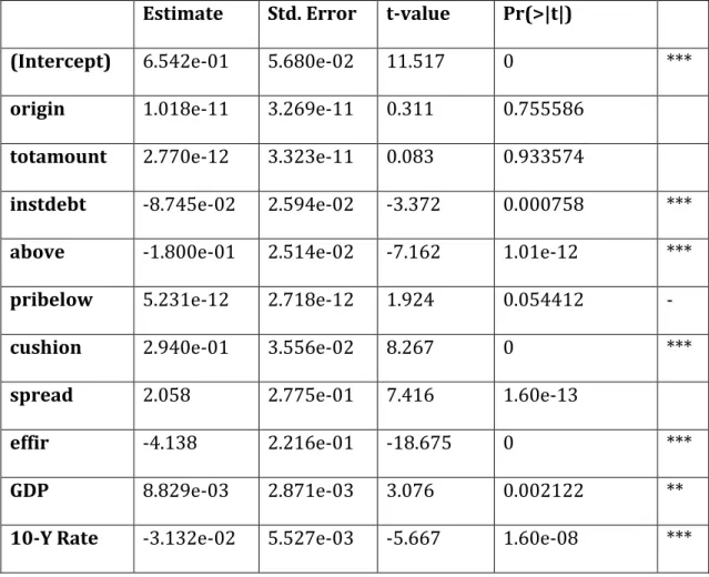
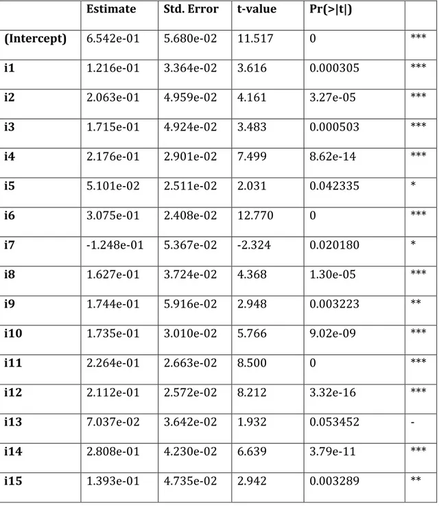
Comparing Table 6 with Table 4, it should be pointed out that, with the exception of NBER's recession indicator (NBER_RI), macroeconomic variables in the model have p-values similar to, or smaller than those displayed previously. The R2 _{is just below 45%.}

Table 6 – The determinants of bond recovery rates given by a least squares regression

(Intercept) 6.542e-01 5.680e-02 11.517 0 ***

origin 1.018e-11 3.269e-11 0.311 0.755586 totamount 2.770e-12 3.323e-11 0.083 0.933574

instdebt -8.745e-02 2.594e-02 -3.372 0.000758 ***

above -1.800e-01 2.514e-02 -7.162 1.01e-12 ***

pribelow 5.231e-12 2.718e-12 1.924 0.054412 -

cushion 2.940e-01 3.556e-02 8.267 0 ***

spread 2.058 2.775e-01 7.416 1.60e-13

effir -4.138 2.216e-01 -18.675 0 ***

GDP 8.829e-03 2.871e-03 3.076 0.002122 **

(26)

NBER_RI 7.559e-02 1.967e-02 3.843 0.000124 *** No. Defaults -3.386e-03 7.076e-04 -4.786 1.79e-06 *** Default Rate 4.047e-02 2.040e-02 1.984 0.047385 * S&P 500 6.267e-03 1.281e-03 4.894 1.05e-06 *** Signif. Codes - 0 (***); 0.001 (**); 0.01 (*); 0.05 (-); 0.1 ( )

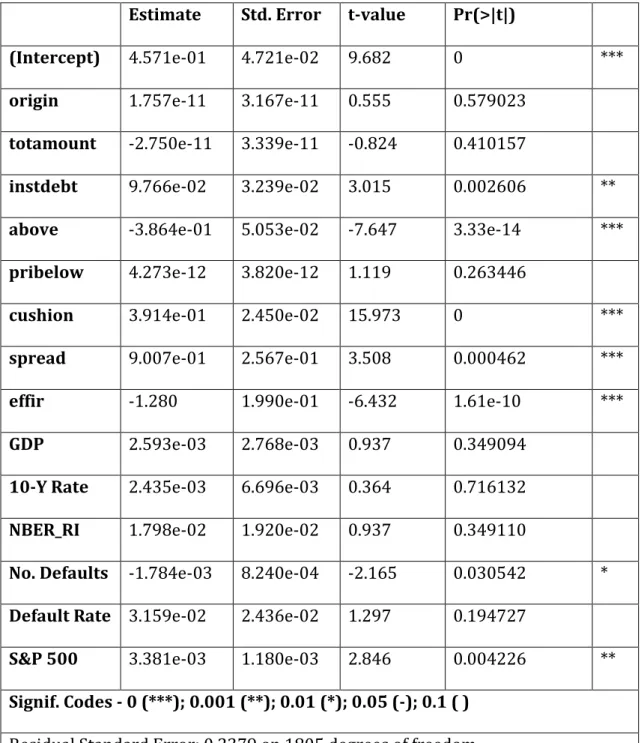
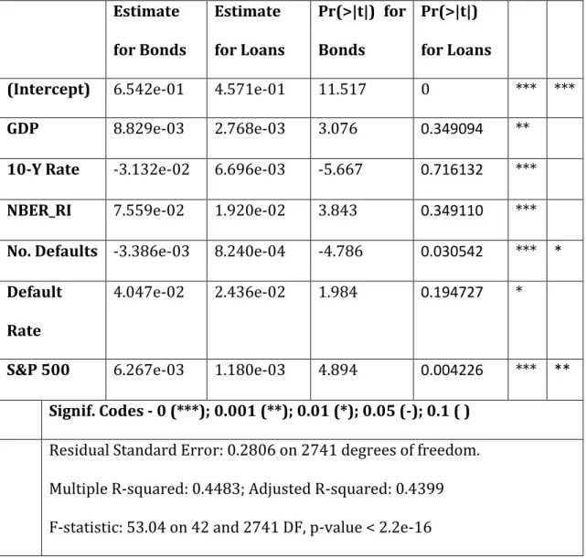
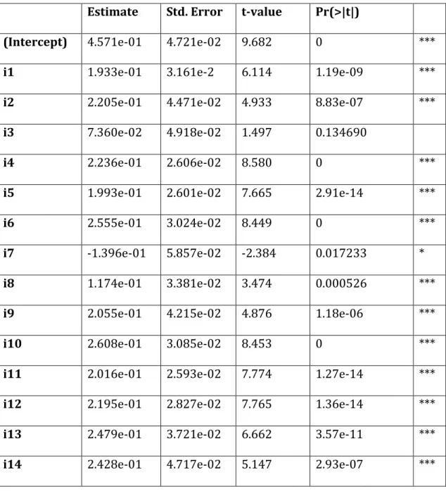
Table 7 displays the determinants of loan recovery rates and Table 8 compares recovery rates for bonds and loans9_{. The first noteworthy issue is that}

the macroeconomic variables are weaker determinants of loan recoveries, especially when compared to bond recoveries. All of them - with the exception of the index S&P 500, which cannot be considered a macroeconomic variable in the strictest definition - exceed typical significance levels, leading us to conclude upon their irrelevance. It should also be noticed that this is not the case with the model's other variables tested. From this, we infer that loans' recovery rates are most likely unaffected by macroeconomic conditions, contrary to what is seen with bond's recovery rates.

This does not defy conventional wisdom on the subject and seems to attest Acharya, Bharath and Srinivasan (2007)'s and Varma & Cantor (2005)'s

9_{Table 8 is abridged, displaying only macroeconomic variables, as the focus of}

this dissertation is on macroeconomic determinants of LGD. No variables were removed from the model.

(27)

statement that loans are more likely to be secured than bonds, leaving them less exposed to market conditions and general macroeconomic circumstances.

Table 7 - The determinants of loan recovery rates given by a least squares regression

(Intercept) 4.571e-01 4.721e-02 9.682 0 ***

instdebt 9.766e-02 3.239e-02 3.015 0.002606 **

above -3.864e-01 5.053e-02 -7.647 3.33e-14 ***

pribelow 4.273e-12 3.820e-12 1.119 0.263446

cushion 3.914e-01 2.450e-02 15.973 0 ***

spread 9.007e-01 2.567e-01 3.508 0.000462 ***

effir -1.280 1.990e-01 -6.432 1.61e-10 ***

GDP 2.593e-03 2.768e-03 0.937 0.349094

10-Y Rate 2.435e-03 6.696e-03 0.364 0.716132 NBER_RI 1.798e-02 1.920e-02 0.937 0.349110

No. Defaults -1.784e-03 8.240e-04 -2.165 0.030542 * Default Rate 3.159e-02 2.436e-02 1.297 0.194727

S&P 500 3.381e-03 1.180e-03 2.846 0.004226 ** Signif. Codes - 0 (***); 0.001 (**); 0.01 (*); 0.05 (-); 0.1 ( )

(28)

Multiple R-squared: 0.3909; Adjusted R-squared: 0.3777 F-statistic: 29.7 on 39 and 1805 DF, p-value < 2.2e-16

Table 8 – The determinants of bond and loans recovery rates: a comparison Estimate for Bonds Estimate for Loans Pr(>|t|) for Bonds Pr(>|t|) for Loans

(Intercept) 6.542e-01 4.571e-01 11.517 0 *** ***

GDP 8.829e-03 2.768e-03 3.076 0.349094 **

10-Y Rate -3.132e-02 6.696e-03 -5.667 0.716132 *** NBER_RI 7.559e-02 1.920e-02 3.843 0.349110 *** No. Defaults -3.386e-03 8.240e-04 -4.786 0.030542 *** * Default

Rate

4.047e-02 2.436e-02 1.984 0.194727 *

S&P 500 6.267e-03 1.180e-03 4.894 0.004226 *** ** Signif. Codes - 0 (***); 0.001 (**); 0.01 (*); 0.05 (-); 0.1 ( )

(29)

4. Conclusions and Future Work

This study shows that macroeconomic variables, as a whole, may be relevant to the evolution of recovery rates and, consequently, to that of loss given default. Interestingly, it suggests the number of default events influences capital recovery, but market default rate is of little consequence.

One question that raised interest and certainly demands further research is the correlation between maturity rates and recovery rates, which, upon statistical testing, was shown to be negative. The reasoning behind this is not evident, and the issue is probably more complex than initially supposed. A possible theoretical argument was presented, but it is likely there are other plausible explanations.

Testing for bonds and loans separately confirmed the notion stated in previous literature (Acharya, Bharath and Srinivasan, 2007; and Varma & Cantor, 2005) that loans are more likely to be secured than bonds, making loans' recovery rates less susceptible to macroeconomic determinants than bonds'.

A macroeconomic variable found to be of particular significance is the National Bureau of Economic Research's recession indicator.

While results obtained by linear estimation should be combined with those emanating from other approaches, it appears that macroeconomic conditions, as a whole, influence loss given default.

Finally, it is concluded linear predictions give a good indication of how macroeconomic variables relate to the dependent variable. It is nevertheless

(30)

possible these correlations - while existent - may not be as high as linear estimation suggests.

(31)

5. References

Acharya, Viral V.; Bharath, Sreedhar T, & Srinivasan, Anand (2007). Does industry-wide distress affect defaulted firms? Journal of Financial Economics 85, 787-821.

Bastos, João A. (2014). Ensemble predictions of recovery rates. Journal of

Financial Services Research 46, 177-193.

Bastos, João A. (2010a). Forecasting bank loans loss-given-default. Journal of

Banking & Finance 34, 2510-2517.

Bastos, João A. (2010b). Predicting bank loans recovery rates with neural networks. CEMAPRE Working Papers 1003.

Bellotti, Tony & Crook , Jonathan (2012). Loss given default models incorporating macroeconomic variables for credit cards. International Journal of

Forecasting 28, 171-182.

Bruche, Max & González-Aguado, Carlos (2010). Recovery rates, default probabilities, and the credit cycle. Journal of Banking and Finance 34, 754-764.

(32)

Caselli, Stefano; Gatti, Stefano & Queri, Francesca (2008). The sensitivity of the loss given default rate to systematic risk: New empirical evidence on bank loans.

Journal of Financial Services Research 34, 1-34.

Dermine, Jean & Neto de Carvalho, Cristina (2006). Bank loan losses-given-default: A case study. Journal of Banking & Finance 30, 1219-1243.

Frye, Jon (2005). A false sense of security. In Altman, Edward; Resti, Andrea & Sironi, Andrea - Recovery rates and loss given default. Risk Books, 2005.

Grunert, Jens & Weber, Martin (2009). Recovery rates of commercial lending: Empirical evidence for German companies. Journal of Banking & Finance 33, 505-513.

Gupton, Greg M. & Stein, Roger M. (2005). LossCalc V2: Dynamic prediction of LGD. Moody's Investor Service.

Jankowitsch, Rainer; Nagler, Florian & Subrahmanyam, Marti G (2014). The determinants of recovery rates in the US corporate bond market. Journal of

Financial Economics 114, 155-177.

Khieu, Hinh D.; Mullineaux, Donald J. & Yi, Ha-Chin (2012). The determinants of bank loans recovery rates. Journal of Banking & Finance 36, 923-933.

(33)

Loterman, Gert; Brown, Iain; Martens, David; Mues, Christophe & Baesens, Bart (2012). Benchmarking regression algorithms for loss given default modeling.

International Journal of Forecasting 28, 161-170.

Papke, Leslie E. & Wooldridge, Jeffrey M. (1996). Econometric methods for fractional response variables with an application to 401(k) plan participation rates. Journal of Applied Econometrics 11, 619-632.

Qi, Min & Zhao, Xinley (2011). Comparison of modeling methods for loss given default. Journal of Banking & Finance 35, 2842-2855.

Varma, Praveen & Cantor, Richard (2005). Determinants of recovery rates on defaulted bonds and loans for North American corporate issuers: 1983-2003.

(34)

Annexes

Annex 1 – Description of the database’s variables Dependent variable:

 Recovery rate – Moody’s calculates recoveries resorting to 3 different methodologies (recommended nominal recovery, family recovery and recommended discounted recovery) and makes a choice on the most appropriate methodology on a case-by-case basis;

Moody’s URD independent variables:

 3 dummy variables – for industry, collateral and instrument type;

 Percentage of obligor’s debt senior to the instrument;

 Percentage of obligor’s debt junior to the instrument;

 Instrument rank within the obligor’s liability structure;

 Issuer’s total debt;

 Instrument’s outstanding amount at default (principal amount plus the accreted amount);

 Debt cushion;

Macroeconomic independent variables:

 Quarterly GDP changes, in USD, chained to 2009 US dollars, seasonally adjusted;

 Monthly 10-year Treasury constant maturity rate, not seasonally adjusted;

 National Bureau of Economic Research (NBER) recession indicator, which uses the binary system to signal recession and growth periods;

(35)

 Total number of US corporate defaults, yearly data;

 US corporate default rate, yearly data;

(36)

Table 1 - Estimation based on a Linear Least Squares Regression

Residuals

Min 1Q Median 3Q Max

-0.89456 -0.20062 -0.00652 0.19409 0.92019

(Intercept) 4.813e-01 4.859e-02 9.905 0 ***

i1 1.627e-01 2.411e-02 6.747 1.70e-11 ***

i2 2.153e-01 3.515e-02 6.124 9.88e-10 ***

i3 1.357e-01 3.658e-02 3.710 0.000209 ***

i4 2.179e-01 2.022e-02 10.774 0 ***

i5 1.271e-01 1.877e-02 6.769 1.46e-11 ***

i6 3.164e-01 1.895e-02 16.695 0 ***

i7 -1.262e-01 4.110e-02 -3.070 0.002153 **

i8 1.491e-01 2.636e-02 5.657 1.64e-08 ***

i9 1.840e-01 3.652e-02 5.038 4.88e-07 ***

i10 2.168e-01 2.229e-02 9.722 0 ***

i11 2.128e-01 1.942e-02 10.961 0 ***

i12 2.128e-01 1.979e-02 10.750 0 ***

i13 1.361e-01 2.726e-02 4.992 6.19e-07 ***

i14 3.101e-01 3.247e-02 9.551 0 ***

(37)

i16 2.144e-01 2.053e-02 10.444 0 ***

i17 1.694e-01 2.684e-02 6.313 2.99e-10 ***

i18 1.139e-01 2.354e-02 4.840 1.34e-06 ***

s1 2.034e-01 4.264e-02 4.771 1.89e-06 ***

s2 1.251e-01 4.257e-02 2.939 0.003311 **

s3 2.369e-02 3.598e-02 0.658 0.510290

s4 1.705e-01 3.559e-02 4.790 1.72e-06 ***

s5 2.799e-02 3.651e-02 0.767 0.443404

s6 1.810e-01 4.222e-02 4.287 1.85e-05 ***

c1 9.248e-02 2.304e-02 4.014 6.06e-05 ***

c2 7.542e-02 2.906e-02 2.595 0.009482 **

c3 1.627e-01 2.992e-02 5.438 5.67e-08 ***

c4 1.143e-01 4.116e-02 2.777 0.005509 **

c5 4.131e-02 2.836e-02 1.457 0.145307

c6 2.416e-02 2.721e-02 0.888 0.374584

instdebt -4.483e-02 2.042e-02 -2.195 0.028185 *

above -1.868e-01 2.186e-02 -8.548 0 ***

pribelow 2.029e-12 2.176e-12 0.933 0.351034

cushion 3.478e-01 2.086e-02 16.674 0 ***

spread 7.772e-01 1.840e-01 4.223 2.46e-05 ***

(38)

GDP 6.410e-03 2.086e-03 3.072 0.002138 ** 10-Y Rate -1.197e-02 4.260e-03 -2.811 0.004963 **

NBER_RI 5.875e-02 1.425e-02 4.212 3.83e-05 ***

No. Defaults -1.770e-03 5.446e-04 -3.249 0.001165 ** Default Rate 8.998e-03 1.590e-02 0.566 0.571489

S&P 500 3.910e-03 9.267e-04 4.220 2.49e-05 *** Signif. Codes - 0 (***); 0.001 (**); 0.01 (*); 0.05 (-); 0.1 ( )

(39)

Table 6 - The determinants of bond recovery rates given by a least squares regression

Residuals

-0.80305 -0.21049 -0.04929 -0.20781 0.90429

(Intercept) 6.542e-01 5.680e-02 11.517 0 ***

i1 1.216e-01 3.364e-02 3.616 0.000305 ***

i2 2.063e-01 4.959e-02 4.161 3.27e-05 ***

i3 1.715e-01 4.924e-02 3.483 0.000503 ***

i4 2.176e-01 2.901e-02 7.499 8.62e-14 ***

i5 5.101e-02 2.511e-02 2.031 0.042335 *

i6 3.075e-01 2.408e-02 12.770 0 ***

i7 -1.248e-01 5.367e-02 -2.324 0.020180 *

i8 1.627e-01 3.724e-02 4.368 1.30e-05 ***

i9 1.744e-01 5.916e-02 2.948 0.003223 **

i10 1.735e-01 3.010e-02 5.766 9.02e-09 ***

i11 2.264e-01 2.663e-02 8.500 0 ***

i12 2.112e-01 2.572e-02 8.212 3.32e-16 ***

i13 7.037e-02 3.642e-02 1.932 0.053452 -

i14 2.808e-01 4.230e-02 6.639 3.79e-11 ***

(40)

i16 2.354e-01 2.665e-02 8.834 0 ***

i17 1.694e-01 3.924e-02 4.317 1.64e-05 ***

i18 5.874e-02 2.992e-02 1.963 0.049706 *

s1 1.764e-01 5.503e-02 3.206 0.001363 **

s2 3.158e-02 3.701e-02 0.853 0.393544

s3 1.602e-01 3.694e-02 4.336 1.50e-05 ***

s4 2.802e-02 3.754e-02 0.747 0.455388 c1 4.590e-02 4.715e-02 0.974 0.330303 c2 7.428e-02 5.055e-02 1.470 0.141802 c3 3.269e-01 1.156e-01 2.828 0.004722 ** c4 -1.936e-01 7.398e-02 -2.617 0.008920 ** c5 -7.133e-03 4.555e-02 -0.157 0.875577 c6 2.182e-02 4.020e-02 -0.543 0.587281

origin 1.018e-11 3.269e-11 0.311 0.755586 totamount 2.770e-12 3.323e-11 0.083 0.933574

instdebt -8.745e-02 2.594e-02 -3.372 0.000758 ***

above -1.800e-01 2.514e-02 -7.162 1.01e-12 ***

pribelow 5.231e-12 2.718e-12 1.924 0.054412 -

cushion 2.940e-01 3.556e-02 8.267 0 ***

spread 2.058 2.775e-01 7.416 1.60e-13

effir -4.138 2.216e-01 -18.675 0 ***

GDP 8.829e-03 2.871e-03 3.076 0.002122 **

(41)

NBER_RI 7.559e-02 1.967e-02 3.843 0.000124 *** No. Defaults -3.386e-03 7.076e-04 -4.786 1.79e-06 *** Default Rate 4.047e-02 2.040e-02 1.984 0.047385 * S&P 500 6.267e-03 1.281e-03 4.894 1.05e-06 *** Signif. Codes - 0 (***); 0.001 (**); 0.01 (*); 0.05 (-); 0.1 ( )

(42)

Table 7 - The determinants of loan recovery rates based on a linear least squares regression

Residuals

-0.82590 -0.11825 0.04039 0.14710 0.78340

(Intercept) 4.571e-01 4.721e-02 9.682 0 ***

i1 1.933e-01 3.161e-2 6.114 1.19e-09 ***

i2 2.205e-01 4.471e-02 4.933 8.83e-07 ***

i3 7.360e-02 4.918e-02 1.497 0.134690

i4 2.236e-01 2.606e-02 8.580 0 ***

i5 1.993e-01 2.601e-02 7.665 2.91e-14 ***

i6 2.555e-01 3.024e-02 8.449 0 ***

i7 -1.396e-01 5.857e-02 -2.384 0.017233 *

i8 1.174e-01 3.381e-02 3.474 0.000526 ***

i9 2.055e-01 4.215e-02 4.876 1.18e-06 ***

i10 2.608e-01 3.085e-02 8.453 0 ***

i11 2.016e-01 2.593e-02 7.774 1.27e-14 ***

i12 2.195e-01 2.827e-02 7.765 1.36e-14 ***

i13 2.479e-01 3.721e-02 6.662 3.57e-11 ***

(43)

i15 3.121e-01 5.413e-02 5.766 9.53e-09 ***

i16 1.886e-01 2.983e-02 6.321 3.27e-10 ***

i17 1.828e-01 3.342e-02 5.469 5.17e-08 ***

i18 2.725e-01 3.832e-02 7.109 1.67e-12 ***

s1 2.080e-02 1.204e-02 1.728 0.084184 -

c1 3.508e-02 2.660e-02 1.319 0.187341

c2 -1.798e-02 3.399e-02 -0.529 0.596872

c3 8.086e-02 3.136e-02 2.578 0.010009 *

c4 1.861e-01 4.497e-02 4.137 3.68e-05 ***

c5 6.258e-03 3.602e-02 0.174 0.862075

c6 -1.820e-02 3.726e-02 -0.488 0.625314

instdebt 9.766e-02 3.239e-02 3.015 0.002606 **

above -3.864e-01 5.053e-02 -7.647 3.33e-14 ***

pribelow 4.273e-12 3.820e-12 1.119 0.263446

cushion 3.914e-01 2.450e-02 15.973 0 ***

spread 9.007e-01 2.567e-01 3.508 0.000462 ***

effir -1.280 1.990e-01 -6.432 1.61e-10 ***

GDP 2.593e-03 2.768e-03 0.937 0.349094

10-Y Rate 2.435e-03 6.696e-03 0.364 0.716132 NBER_RI 1.798e-02 1.920e-02 0.937 0.349110

(44)

Default Rate 3.159e-02 2.436e-02 1.297 0.194727

S&P 500 3.381e-03 1.180e-03 2.846 0.004226 ** Signif. Codes - 0 (***); 0.001 (**); 0.01 (*); 0.05 (-); 0.1 ( )

Macroeconomics determinants of loss given default

Macroeconomic Determinants of Loss Given Default

João Afonso Bastos

Henrique Sousa de Azevedo

Macroeconomic Determinants of Loss Given Default

Declaration of Originality

Acknowledgements

Abstract

Table of Contents

1. Introduction

2. Dataset description

3. Results

4. Conclusions and Future Work

5. References

Annexes