Terms of trade, macroeconomic dynamics and default decisions

(1)

FUNDAÇÃO GETULIO VARGAS ESCOLA DE ECONOMIA DE SÃO PAULO

THIAGO LUIZ CURADO

TERMS OF TRADE, MACROECONOMIC DYNAMICS AND

DEFAULT DECISIONS

(2)

THIAGO LUIZ CURADO

TERMS OF TRADE, MACROECONOMIC DYNAMICS AND

DEFAULT DECISIONS

Dissertação apresentada à Escola de Economia de São Paulo da Fundação Getulio Vargas, como requisito para obtenção do título de Mestre em Economia

Campo de Conhecimento: Macroeconomia Internacional

Orientador: Prof. PhD. Bernardo Gui-marães

(3)

Curado, Thiago Luiz.

Terms of Trade, Macroeconomic Dynamics and Default Decisions / Curado, Thiago Luiz. - 2015.

36 f.

Orientador: Bernardo Guimarães

Dissertação (mestrado) - Escola de Economia de São Paulo. 1. Macroeconomia. 2. Termos de troca. 3. Mercados emergentes. I. Guimarães, Bernardo. II. Dissertação (mestrado) - Escola de Economia de São Paulo. III. Título.

(4)

THIAGO LUIZ CURADO

TERMS OF TRADE, MACROECONOMIC DYNAMICS AND

DEFAULT DECISIONS

Dissertação apresentada à Escola de Economia de São Paulo da Fundação Getulio Vargas, como requisito para obtenção do título de Mestre em Economia

Campo de Conhecimento: Macroeco-nomia Internacional

Orientador: Prof. PhD. Bernardo Gui-marães

Data de Aprovação: / /

Banca examinadora:

Prof. PhD. Bernardo Guimarães (Orientador) FGV-EESP

Prof. PhD. Luis Fernando Araujo FGV-EESP

(5)

Agradecimentos

Agradeço ao meu orientador, Professor Bernardo Guimarães. Suas contribuições foram essenciais para construção deste trabalho. Além disso, nossas conversas constituíram cons-tante fonte de inspiração.

Agradeço aos meus pais, Luiz Alberto e Maria Lúcia, por terem acredito em mim desde as primeiras etapas. Agradeço aos meus irmãos, Ana e Marcelo, pelos exemplos de vida.

Agradeço à minha namorada, Regiane Sousa, por toda paciência e companhia ao longo destes anos de mestrado. Agradeço também a Leopoldo Gutierre, que além de grande amigo prestou inestimáveis contribuições ao longo de diversas etapas.

(6)

ABSTRACT

There is substantial evidence that terms of trade behavior are relevant to understand both the macroeconomic dynamics and the default risk of emerging markets. Nevertheless, the literature of sovereign debt that follows Eaton and Gersovitz (1981) and Arellano (2008) has not yet adequately explored the connections between terms of trade and default incen-tives. We advance in this ﬁeld, introducing terms of trade volatility to the model proposed by Mendoza and Yue (2012), where the sovereign debt decisions are linked to a general equilib-rium model for the domestic economy. We ﬁnd that an economy that faces stochastic terms of trade innovations can produce a consumption variability that highly exceeds the output variability, which is a key stylized fact of emerging markets business cycles. Our exercises also show that default episodes are driven by sudden shifts in the terms of trade but are no necessary related with bad times.

(7)

RESUMO

A evidência empírica aponta que Termos de Troca é uma variável relevante tanto para dinâmica macroeconômica como para o risco de default em países emergentes. No entanto, a literatura de dívida soberana baseada nos trabalhos de Eaton and Gersovitz (1981) e Arel-lano (2008) ainda não explorou de forma adequada as conecções entre a dinâmica de termos de troca e incentivos ao default. Nós contribuímos nessa área, introduzindo volatilidade de Termos de Troca no modelo proposto por Mendoza and Yue (2012), no qual as decisões de dívida soberana são vinculadas à um modelo de equilíbrio geral para a economia doméstica. Nós encontramos que uma economia exposta à volatilidade dos termos de troca consegue produzir uma variabilidade do consumo que supera signiﬁcativamente a variabilidade do produto, característica que constitui um fato estilizado chave de business cycles de países emergentes. Nossos exercícios também mostram que decisões de default são geradas por mudanças bruscas nos termos de troca, mas não necessariamente estão vinculados à estados ruins da economia.

(8)

Introduction

There is substantial evidence that Terms of Trade1 _{behavior are relevant to understand both}

the macroeconomic dynamics and default risk of emerging markets. Despite this indication, the literature of sovereign debt that built on the seminal work of Eaton and Gersovitz (1981) has not yet adequately exploited the connections between Terms of Trade - ToT from now on- and default decisions.

We advance in this field by introducing ToT innovations to Mendoza and Yue (2012) model. In their model, default costs are endogenously determined, arising because domestic producers lose access to international credit and are obligated to reduce the utilization of imported input in the production process. For the stochastic ToT process, the intuition is as follows: when the country observes a worsening in ToT, private agents reduce the amount of imported inputs used in the production process. Thus, the loss of efficiency and product contraction in default episodes will be smaller the lower the ToT are. Similarly, in case of favorable ToT, the share of imported inputs used in the production tends to be higher, raising the costs of being excluded from international financial markets.

By applying this approach, we have now a modeled mechanism by with ToT aﬀects allo-cation plans and, through this, default incentives and spreads. Moreover, we can understand our work in two (complementary) ways. On one hand, we study sovereign debt episodes in a model where default costs are endogenously determine by allocation plans that, in turn, answers to the business cycles. On the other hand, we analyze the macroeconomic dynamics of emerging markets with a structure where spreads are endogenously determined by the probability of default.

In a broad sense, our results show that ToT fluctuations can substantially affect incen-tives to default and, thus, spreads behavior in emerging markets. Moreover, we find that ToT volatility can help to explain two key stylized facts of emerging markets that are not well addressed if we only take into account productivity shocks. First, it can generate a consump-tion variability 1.55 times higher than income volatility, closely matching the empirical data. This result comes from the fact that ToT produces a small GDP variance but a high trade balance volatility. Second, in the stochastic ToT model only 71 % of default happens in "bad times", approximating Tomz and Wright (2007) estimates of 61.5 %. In fact, since in our model is the combination of the ToT realization and the debt level that defines the incentive to repay its debt, defaults episodes are triggered by large ToT contractions, with the level of

1

(10)

Introduction 10

this variableper se not being a primary driver for default decision. These innovations in our results come from the fact that ToT affect default incentives through a substitution effect over the imported and domestic varieties of intermediate goods while a productivity shock impact production in a more directly way, affecting the demand for every production factor. Turning now to empirical evidence, Mendoza (1995) and Kose (2002) find that ToT in-novations account for nearly half of actual GDP volatility for emerging markets. This char-acteristic is related to large fluctuations in relative prices faced by this group of countries. According to Baxter and Kouparitsas (2006), ToT has a standard deviation of 19% per year in emerging markets, more than twice the estimated for developed countries (9 %), attribut-ing this pattern to the heavy reliance on commodity’s exports, whose prices are more volatile than manufactured goods. Reinforcing this view, Broda (2004) highlights that emerging mar-kets are particularly exposed to relative price oscillations since they have very little influence on their exportation prices.

The literature also finds that ToT fluctuations can be an important predictor of sovereign default and interest rate spreads in emerging markets. Hilscher and Nosbusch (2010) find that one standard deviation increase in terms of trade volatility is associated with a rise of 164 basis points (EMBI) in spreads (half of the spreads empirical standard deviation). Min et al. (2003) find that 1% improvement in ToT reduces yield spread by 1.02%. Moreover, some works focus on particular episodes of spread volatility induced by heavily ToT drops. For instance, Caballero (2003) comments Chile experience during Asian crises; Sturzenegger and Zettelmeyer (2006) analyze Russian default of 1998; and Hatchondo, Martinez and Sapriza (2007) comments Ecuador’s sovereign default in 1999.

(11)

renego-Introduction 11

tiation protocol designed by a benevolent planner when two countries renegotiate with the same lender. Arellano et al. (2012) investigate mature composition and term structure of interest rate spreads, working with a model with endogenous default and multiple maturities of debt.

A second ﬁeld of the literature developed general equilibrium models of business cycles for emerging markets. Nevertheless, theses works treat default episodes and, thus, interest rate as an exogenous variable. For example, see Neumeyer and Perri (2005) and Uribe and Yue (2006). The research here could explore how ToT ﬂuctuation impact factor allocations, but were not able to connect this with default incentives and interest rate behavior.

However, a solution to the disconnection between this two literature has been proposed by Mendoza and Yue (2012), who built a general a general equilibrium model of both sovereign default and business cycles. With this framework, we can study the interactions between ToT, factors allocations and default incentives. Moreover, since spreads are also endoge-nously determined, we can explore the interactions between ToT ﬂuctuation and interest rates behavior.

(12)

12

1 Model

Figure 1 gives a model overview. We have four domestic agents. Households (1) choose consumption and labor supply. Final goods producers (2) uses labor and an intermediate good composed of a mix of imported and the domestic inputs produced by Intermediate Goods Firms (3), which in turn uses only labor as input. The Sovereign Government (4) makes the ﬁnancial link with the rest of the world. Time is discrete, and every good in is nonstorable.

Figure 1: Model Overview

md

m∗ Final Goods

Producers Domestic Input

Producers

Households

Rest of

the World Government

Import

wages,goods Lf

bt+1

bt(1 +rt)

Transfers Taxes

(13)

Chapter 1. Model 13

1.1 Households and Firms

Households choose consumptioncand labor supplyL in order to maximize a time-separable utility function, such that:

E ct,Lt

" X

βt(c−L

ω_/w₎1−σ₋₁

1−σ

#

s.t. ct=wtLt+πtf +πmt +Tt (1.1)

where w is the wage, Tt is the transfer received from the government, πf and πm are

the profits received from firms andσ is the coefficient of relative risk aversion. They cannot borrow from abroad, but the government borrows, pays transfers and makes default decision internalizing their utility.

Let’s deﬁne now ﬁrm’s behavior. First, Domestic Input Producers uses only labor Lm _to

produce the domestic inputmd_{. The intermediate sector productivity is given by the constant}

parameter A while γ deﬁne the labor share in production. Domestic Input Producers sell this input to ﬁnal goods producers at a given pricepm _{and pay wages to households.}

max

Lm t

πm_t =pm_t A(Lm_t )γ₋_w

tLmt (1.2)

Second, Final Good Producers use labor Lf_{, a compound intermediate good} _M _{and a}

time-invariant capital stock k to produce the ﬁnal y good consumed by households. Their production function is a standard Cobb-Douglas:

yt =ε

M(md_t, m∗

t) αM

(Lft)αLkαk (1.3)

where ε is the productivity of the economy (TFP hereafter). In our simulations, we ﬁx ε= 1. Finally,Mtis a mix of intermediate goods determined by a CES Armington aggregator

that combines domestic inputmd

t whit the j imported inputs m∗t varieties, such that

Mt= [λ(mdt)µ+ (1−λ)(m∗t)µ]1/µ (1.4)

and

m∗ ₌

   θ ˆ 0 m∗ j _νν −1 dj+ 1 ˆ θ m∗ j _νν −1 dj   

ν−1

ν

(1.5)

where λ is the Armington weight of domestic inputs, µ is the Armington curvature pa-rameter andν is the Dixit-Stiglitz curvature parameter.

(14)

are not able to import this fraction θ, and have to reorganize production with domestic inputs. The loss in eﬃciency that arrives from this forced resource reallocation is the key mechanism by which default costs are endogenously determined.

Notice that we have two fonts for this inefficiency. The first one comes from imperfect substitution between domestic and imported varieties, as defined by equation 1.4. The elas-ticity of substitution is given by ηmd_,m∗ =

1

µ−1

. Also, a second ineﬃciency comes from the

substitution across imported varieties, with the elasticity of substitution being deﬁned by ηm∗

j =

1

ν−1 .

Taking wages wt and pricesp∗, pm,pf and interest rate r∗ as given, ﬁnal goods producers

solve:

max

Lf_t,md t,m∗t

πft =pfMtαM

Lft αL

kαk ₋_r∗

t θ

ˆ

0

p∗

jm∗jtdj−

1

ˆ

0

p∗

jm∗jtdj −pmt mdt −wtLft (1.6)

To close this section, we deﬁne the price ofm∗

t as the CES price index

p∗(r∗

t) =    θ ˆ 0 p∗

j(1 +r∗t) _νν −1 + 1 ˆ θ p∗ j _νν −1 dj   

ν−1

ν

which implies that the price in case of default (ﬁnancial autarky) is

p∗ aut=    1 ˆ θ p∗ j _νν −1 dj   

ν−1

ν

Following Mendoza and Yue (2012), we deﬁne pf _{as the numeraire price while} _pm _is

en-dogenously determined in equilibrium. We introduce ﬂuctuations in the relative price of imported inputs, p∗_{. More precisely, these prices face Markov shock with transition} proba-bility distribution functionz(p∗

t|p∗t−1). Notice from (1.5) that if the economy faces a positive

shock on p∗_{, ﬁnal goods producers will choose less imported inputs. Consequently, the cost} of an eventual default will be lower.

From now own, we are going refer to ToT shocks, with the following deﬁnition in mind: Definition 1. Terms of Trade (ToT) are defined as the ratio of final goods prices to import prices, i.e.,

T oT := p

f

p∗ = 1 p∗

(15)

1.2 Removing the Wealth Effect

Following Mendoza and Yue (2012), we work with a GHH speciﬁcation1 _{for household’s utility}

function. This choice has critical implications for the model since it removes any wealth effect on labor supply. If we did not remove the wealth effect, we would produce a countercyclical behavior of labor supply that is not observed in emerging markets business cycles data. For our model, this implies that labor supply decisions areindependent of the current debt level. To see this, notice that the government is going to pay its debt through taxT. This variable affects household’s consumption level, but not their labor decision.

To formalize this discussion, let’s deﬁne Ω as non-default/default state space, i.e.,

Ω = [N onDef ault, Def ault] (1.7)

Also, deﬁne Bt as the sovereign government net debt position at time t. More precisely,

every period the government pays a debt bt contracted at t−1, and issues a discount bond

with face value ofqtbt+1, whereqis given by the international risk-free asset plus the country

spread. Therefore, we have that

Definition 2. At every period t, the net debt position Bt is given by the Bt:=−bt+qbt+1

If Bt > 0, the economy is absorbing external resources. This fact implies that the

gov-ernment is going to make positive transfers to households, i.e., Tt > 0. If Bt < 0, the

economy must send resources to external lenders. In order to gather necessary resources, the government tax households, i.e., Tt <0.

From this deﬁnition and the previous discussion about GHH utility function consequences, we can write thatc=c(T oT,Ω, B) and L=L(T oT,Ω). This means that we can determine labor, and all other factor allocation of the economy, conditional only on default state and ToT realization. For this reason, we can fully determine the supply side of the economy without taking into account the economy net debt position. Nevertheless, Bt determines

transfer/taxation made by the sovereign government. Therefore, household’s consumption is a function of the net debt position (altogether with ToT and default state). In sum, the debt level is a key variable to agent’s welfare, even though it does not aﬀect the supply side of the economy.

1

(16)

1.3 GDP and Trade Balance

We make now some additional deﬁnitions that are going be useful in Result’s section. First, following Mendoza and Yue (2012), we calculate economy GDP as the production of ﬁnal goods minus the cost of imported inputs, i.e.,

gdpt:=yt−p∗tm∗t (1.8)

.

Additionally, using profit’s definitions in equations (1.2) and (1.6) together with equation (1.8) we can derive an income approach definition for GDP:

gdpt =πtm+π f

t +wtLt (1.9)

Next, a basic national account identity allows to deﬁne the trade balance as

tbt:=yt−p∗m∗−ct (1.10)

Additionally, from the model construction we have that the trade balance equals the net debt positionBt, i.e.:

tbt =−bt+qtbt+1 =Bt (1.11)

Substituting household’s budget constraint and using equation (1.10) and (1.11 we get that:

Bt =tbt=−Tt (1.12)

i.e., the amount of transfers/taxation made by the government equals the trade balance and the opposite of the economy net debt positionBt.

Finally, these deﬁnition clarify why we have gdp=gdp(T oT,Ω), tb=tb(T oT,Ω, Bt) and c=c(T oT,Ω, Bt), i.e., GDP depends only on ToT stochastic realization and the default state

while trade balance and, thus, consumption depends additionally on net debt position of the economy.

1.4 Equilibrium in Factor Markets and Production

(17)

Take as given interest rate r∗

t and a stochastic realization of p∗. The corresponding

(partial) equilibrium factor allocations are given by the values of hm∗_{, m}d_{, L}f_{, L}m_{, L}i _and

[pm_{, w}_{] that solve the following nonlinear system:}

αMεtkak[λ(mdt)µ+ (1−λ)(m∗t)u](αM−µ)/µ(Lft)αL(1−λ)(m∗t)µ−1 =P∗(r∗t) (1.13)

αMεtkak[λ(mdt)µ+ (1−λ)(m∗t)u](αM−µ)/µ(L f

t)αLλ(mdt)µ−1 =pmt (1.14)

αLεtkak[λ(mdt)µ+ (1−λ)(m∗t)u](αM)/µ(L f

t)αL−1 =wt (1.15)

γpm_t A(Lm_t )γ−1 ₌_w

t (1.16)

Lω−1

t =wt (1.17)

Lft +Lmt =Lt (1.18)

A(Lm_t )γ₌_md

t (1.19)

Equations (1.13), (1.14) and (1.15) comes from the ﬁrst stage of Final goods Producers’ optimization problem while (1.16) comes from the proﬁt maximization problem of Intermedi-ate Good Producers. Equation(1.17) is the optimality condition for labor supply while (1.18) is an aggregate resource restriction. Finally, equation (1.19) is a market clearing condition for intermediate goods market.

1.5 Sovereign Government

We now deﬁne the dynamic problem faced by the Sovereign Government. Financial markets are incomplete, bonds are non-state contingent and have a one-period maturity. For every periodt that the economy is in non-default state, the government faces a value functionVnd

(18)

the control variable is the new discounted debt issued,bt+1. In this case, in next period the

government will face a value function Vnd _{again. From this, we can deﬁne}

Vnd(bt, T oTt) = max bt+1

{u[ct(T oTt,Ωt, Bt)−g(L(T oTt,Ωt))] +βE[V(bt+1, T oTt+1)]} (1.20)

where

V(bt, T oTt) = max n

Vnd₍_b

t, T oTt), Vd(T oTt) o

(1.21) We deﬁned V(·) to explicit the fact that in next period the government is going be able to default or to repay its debt. Also from this deﬁnition we can see that the government will repay its debt if and only if Vnd _{> V}d_.

Finally, if the economy chooses to default, debt level goes to zero and the economy is excluded from international ﬁnancial markets. Therefore, the value function faced by the sovereign government, Vd_{, can be expressed as}

Vd(T oTt) =u[ct(T oTt,Ωt,0)−g(L(T oTt,Ωt))]+β(1−φ)EVd(T oTt+1)+βφE[V(0, T oTt+1)]

(1.22) When the economy is in a default state, instant utility is given by u(·). Notice that consumption in default times is diﬀerent from non-default ones for two reasons. First, net debt position Bt goes to zero, which implies that the government transfer/taxation Tt that

enter the household’s budget constraint is also equals zero; in other words, household’s con-sumption is now defined exclusively by their current income, determined by the sum of wages and profits paid by domestic firms (see equation 1.1). Second, default state Ωt affects the

production side through the exclusion mechanism of inputs importation. On next period, the economy may reenter international ﬁnancial markets with a probability φ. If this hap-pens, the Sovereign Government will face the non-default value function with bt = 0, i.e., V(0, T oTt+1). Otherwise, the economy remains in the default state.

1.6 Foreign Lenders

To close the model, there is a continuum of risk-neutral international lenders with full infor-mation, operating in perfectly competitive market. Given an opportunity cost ofr∗_{, derived} from risk-free asset, zero proﬁts condition at equilibrium implies that:

qt(bt+1, T oTt) =      1

1+r∗, if bt+1 ≥0

1−pt(bt+1,T oTt)

1+r∗ otherwise

(19)

1.7 Recursive Equilibrium

In the following equilibrium deﬁnition, we again strictly follow Mendoza and Yue (2012), just changing the stochastic variable of interest.

The model’s recursive equilibrium is given by: (i) a decision rule bt+1(bt, T oTt) for the

sovereign government with associated value functionV(bt, T oTt), consumption and transfers

rules c(bt, T oTt) and T(bt, T oTt), default set D(bt), and default probabilities P r(bt+1, T oTt);

and (ii) an equilibrium pricing function for sovereign bonds q∗₍_b

t+1, T oTt) such that:

1. Givenq∗₍_b

t+1, T oTt), the decision rulebt+1(bt, T oTt) solves the social planner’s recursive

maximization problem (1.21).

2. The consumption plan c(bt, T oTt) satisﬁes the resource constraint of the economy.

3. The transfers policyT(bt, T oTt) satisﬁes the government budget constraintT(bt, T oTt) = qt(bt+1, T oTt)bt+1−bt.

4. Given D(bt) and P r(bt+1, T oTt), the bond pricing function q∗(bt+1, T oTt) satisﬁes the

arbitrage condition of foreign lenders (1.23).

1.8 Timing

We explain now the timing of decisions. At the beginning of each period, Terms of Trade realization is observed, and private agents deﬁne allocations plans, conditional on default state. Given this allocation plans and the amount of debt brought from the previous period, the sovereign government chooses to repay its debt or to default, internalizing household’s welfare.

If the economy repays its debt, the government decide how much to borrow depending on spreads. The spreads, in turn, are determined by ToT realization and the amount of debt chosen. Labor supply, intermediate goods demand, and GDP are determined independently of spreads and the debt level. Finally, consumption is determined by the sum of GDP and Trade Balance (that, in turn, depends on debt), altogether with government taxation and transfers. On the next period, the process starts again, with agents observing ToT.

(20)

20

2 Quantitative Results

We begin this section briefly presenting our solution methodology. The first step of our work was to write this code and replicate all results reported by Mendoza and Yue (2012). Next, we solve the model for ToT innovation. By doing this, we were able to explore the drivers for differences in results from the models.

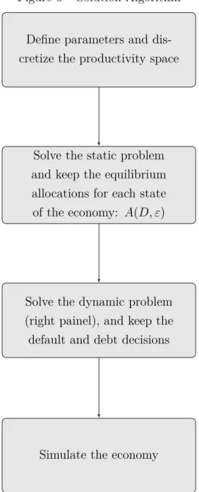
Figure 6 on Appendix resumes our procedures. First, we deﬁned parameters and dis-cretized ToT space. Table A on Appendix shows parameters calibration used and the respec-tive target from Argentina’s Data. Mendoza and Yue (2012) brings an extensive description of the calibration and its implications for the results.

Next, we solved the static problem through numerical simulation. With this, we got a map of equilibrium allocations for each possible state of the economy, i.e., for every possible (T oT,Ω) combination.

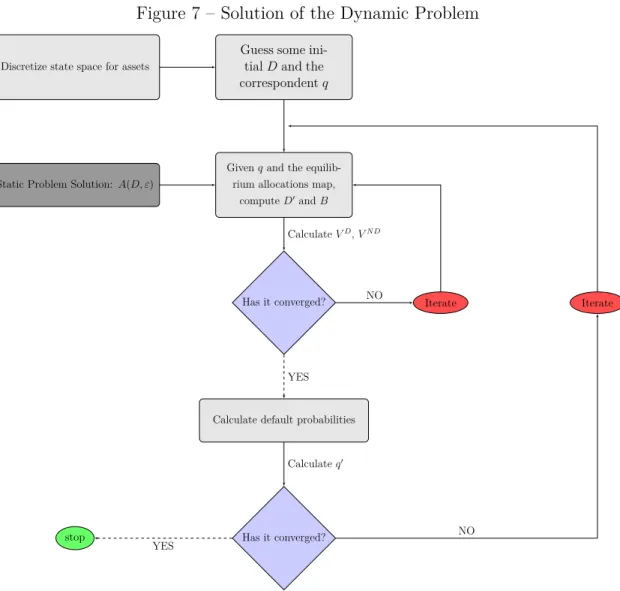
In the third step, we solved the dynamic problem of the Sovereign Government. Figure 7 in Appendix illustrates our solution algorithm. From this, we got debt and default decision for all possibles states of the economy. With this second map in hand, in the last step we simulate the economy, running 2000 simulations, each with 500 periods (the ﬁrst 100 observations were dropped).

(21)

Chapter 2. Quantitative Results 21

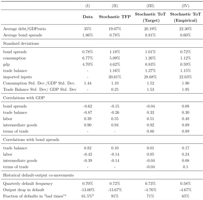
Table 1 – Statistical Moments in the Simulations and in the Data

(I) (II) (III) (IV)

Data Stochastic TFP Stochastic ToT Stochastic ToT (Target) (Empirical)

Average debt/GDPratio 35% 19.07% 20.19% 22.30%

Average bond spreads 1.86% 0.78% 0.81% 0.60%

Standard deviations

bond spreads 0.78% 1.18% 1.01% 0.72%

consumption 6.77% 5.09% 1.26% 1.12%

gdp 4.70% 4.62% 0.83% 0.59%

trade balance - 1.16% 1.27% 1.15%

imported inputs - 20.61% 28.68% 22.63%

Consumption Std. Dev./GDP Std. Dev. 1.44 1.10 1.52 1.90

Trade Balance Std. Dev/ GDP Std. Dev - 0.25 1.53 1.95

Correlations with GDP

bond spreads -0.62 -0.15 -0.04 0.08

trade balance -0.87 -0.26 0.33 0.30

labor 0.39 0.55 0.51 0.48

intermediate goods 0.90 0.94 0.92 0.89

terms of trade - - 0.80 0.89

Correlations with bond spreads

trade balance 0.82 0.10 0.01 0.17

labor -0.42 -0.14 0.05 0.24

intermediate goods -0.39 -0.14 -0.04 0.08

terms of trade - - -0.04 0.1

Historical default-output co-movements

Quarterly default frequency 0.70% 0.72% 0.73% 0.58%

Output drop in default -13.00% -13.67% -4.76% -4.67%

Fraction of defaults in "bad times"a _61.5%b _91% _71% _65%

a

We consider "bad times" as periods when the stochastic variable realization is bellow its mean level.

b

Tomz and Wright (2007) historical cross country estimate

2.1 Same Quarterly Default Frequency (Column III)

(22)

economy is more closed and, therefore, more protected from default costs. To understand this diﬀerence, notice that when the economy faces adverse ToT shocks, it responds substituting imported inputs for domestic varieties. In TFP process, however, lower TFP realizations reduces the demand for both domestic and imported varieties of inputs since all production factor becomes less productive.

The last line of Table 1 shows the historical co-movements between default and GDP. We define periods when the stochastic variable is bellow (above) its mean level as "bad times" ("good times"). Using this definition, we find that in the stochastic ToT model 71 % of default episodes happens in bad times, a much lower percentage than the one find in the stochastic TFP model (91%).1_{. Our result is consistent with the estimates of Tomz and Wright (2007),}

who ﬁnd that only 61.5 % happens with GDP bellow trend.2

Going further, we conclude that defaults in our simulations are triggered by contractions of ToT, with the level of the stochastic variableper se not being a primary factor in default decisions. Indeed, it is the combination of ToT realization and debt level that deﬁnes whether or not the economy chooses to default. For this reason, we can observe default episodes in "good times"if the economy is suﬃciently indebted. To generate such a high debt level, the economy must have faced an even greater realization of ToT in the previous period. Likewise, the economy can stand long periods of ToT (and GDP) bellow trend without choosing to default. This scenario is possible if the path through this lower levels of the stochastic variable is relatively smooth. Indeed, notice that since the distribution of the stochastic ToT is centered at its mean level, the percentage found for the ToT simulation of defaults in bad times being greater than 50% is a consequence of the fact that severe shocks more commonly drives logarithm of TOT to levels below zero.

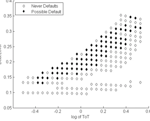
To illustrate this last argument and how default decisions are triggered with stochastic ToT, Figure (1) maps default decisions points for each combination of ToT and debt level (contracted over the previous period). Every period, the sovereign government observes the joint realization of these two variables, and then decides to default (black ﬁlled diamonds) or to repay its debt (empty diamonds).3 _{Again, we can see that our simulation can produce}

1

Mendoza and Yue (2012) detrend GDP series using a HP filter, defining "bad times" as years with GDP below trend. Using this proceeding, we were able to replicate the 83% of default in bad times reported in Mendoza and Yue (2012). For the ToT case, this method generates 88% of default in bad times. Nevertheless, we understand that it is not necessary to use any filter method: since the only font for GDP oscillations in both simulations is the stochastic variable realization, we have a direct and perfect measure of bad and good times

2

The statistics reported by Tomz and Wright (2007) are based on annual data. For this reason, Mendoza and Yue (2012), annualize their data in order to calculate this historical output-default co-movement. Nevertheless, we choose to report default frequency using the original quarterly data generated by the simulations since default decisions are quarterly considerations on the model. For this reason, annualizing the data add unnecessary noise to bad times /god times computation.

3

(23)

default with ToT above mean, depending on the debt ﬂow. For concreteness, suppose that the economy at a timetfaces a high realization of ToT; for example, equal to 0.4. This implies a high demand for imported inputs since their prices are relatively small. In addition, since the high realization of ToT reduces default probability, we observe a reduction of spreads. Both eﬀects induce the economy to contract more debt. Suppose now that the economy faces an adverse shock, with ToT going to 0.2. Notice that the economy may choose to default even though we are in good times, depending on the debt level contracted during the previous period (when times were even better).

Figure 1 – Debt Level, ToT Realization and Default Decisions

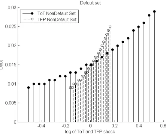
Next, ﬁgure 2 shows non-default areas for the stochastic ToT and TFP cases. For highers realizations of the stochastic variable, the economy can face highers contracted debt without choosing to default. Nevertheless, for each possible realization of the stochastic variables, there are debt levels that trigger default.

(24)

Figure 2 – Default and non-default Regions

Figure 2 also helps to understand why we need a greater standard deviation of ToT to generate the same quarterly default frequency induced by TFP shocks. First, notice that ToT non-default area is ﬂatter. This implies that the minimum debt level that triggers default is more sensible to TFP than ToT oscillations. Therefore, in order to generate the same default frequency, we need a higher standard deviation of the ToT process, such that we can observe shifts in ToT space of suﬃcient magnitude to make the debt level unsustainable.

The model with ToT shocks can produce a consumption variability that exceeds output variability, closely matching the data. More precisely, we generate a standard deviation for consumption 1.52 times greater than the statistic ﬁnd for GDP, which is close to the 1.44 from Argentina’s Data. The stochastic TFP process generates a relation of 1.05. As pointed out by Mendoza and Yue (2012), a consumption volatility that highly exceeds output variability is a key regularity found for emerging markets business cycles.4 _{Neumeyer and Perri (2005)}

and also emphasizes this point. The authors document the relation between real interest rates and business cycles in emerging markets, using a quarterly database for ﬁve emerging

4

(25)

markets (including Argentina) and ﬁve developed countries.5 _{One of their main ﬁndings is}

that "consumption tends to be more volatile than output in emerging economies while it is roughly as volatile as output in developed economies". They estimate that the relation between consumption and income variability is on average equal to 1.30 or 1.71 for emerging markets, depending on whether or not we include government consumption on computation.6

Our result comes from the fact that, relatively to the TFP case, the stochastic ToT model produces a much lower GDP volatility, but at the same time generates a higher trade balance volatility. In fact, the standard deviation of GDP drops from 4.62% to 0.83% while the trade balance standard deviation increases from 1.16% to 1.27%. The first fact happens since TFP has a much larger impact on the supply side of the economy than ToT fluctuations. Nevertheless, ToT innovations can generate significant volatility in imported inputs demand and bond spreads. As a consequence, we can generate trade balance volatility that is even higher than the one produced in the TFP case. Finally, trade balance variance implies that the drop in consumption volatility (from 5.09% to 1.26%)is not as significant as the fall observed for GDP.

Concerning the GDP, notice that, given the default state, there is a univocal relationship between GDP and the stochastic realization. This implies that the stochastic variable insta-bility fully determines GDP volatility. Thus, the drop in GDP volatility comes from the fact that TFP innovations have a much higher impact on GDP than ToT shocks.

The high trade balance volatility comes from its heavy reliance on economic history. More precisely, trade balance depends on level of indebtedness that, in turns, depends on ToT history. Formally, tb = tb(T oT, Bt,Ω), i.e., trade balance is a function of net debt

position, additionally to current ToT level. The essential fact here is that ToT realization can generate a volatility of trade balance components that are not distinct in magnitude from the ones produces by the stochastic TFP model. More precisely, the TFP model generates standard deviations of bond spreads and imported inputs of 1.18% and 20.61% while the Tot model produces 1.01% and 28.68%.

Figures 3 and 4 illustrate the previous discussion with data from our simulations. The left panel of Figure 3 shows consumption and GDP realizations against ToT while the right panel plot Trade Balance realizations. As we can see, GDP is uniquely determined while trade balance and consumption values depend on net debt position of the economy. Since

5

Emerging markets: Argentina, Brazil, Korea, Mexico and Philippines. Developed economies: Australia, Canada, Netherlands, New Zealand and Sweden. The sample comprehends the period between the third quarter of 1983 and the last quarter of 2001 for Argentina and the developed economies. For the other four emerging markets, the data starts in the first quarter of 1994.

6

(26)

the debt contracted in the previous period is determined by the stochastic realization of (any) ToT from the previous period, we have a lot of possibles values for consumption and trade balance for each current ToT realizations. To stress this question, Figure 4 shows GDP, consumption and trade balance when we fix the debt contracted during the previous period. More precisely, we have thatb1 < b2 < b3 < b4 As we can see the consumption and the trade

balance are uniquely determined for each ToT realization, given the contracted debt level and the default state (we have now policy functions that depend on only one variable, since we ﬁxed the debt level and the default state). Moreover, for a given ToT realization, a higher debt level implies a lower consumption and higher trade balance.

(27)

Figure 4 – Trade Balance and Consumption against ToT for a ﬁxed debt

As we noticed in Section 1.2, it is important to remove the wealth eﬀect on labor sup-ply, otherwise producing a countercyclical behavior of the labor supply that is not observed in emerging markets business cycles data. This implies that the debt level is not a rele-vant variable for resource allocation decisions and, therefore, for the GDP determination. Nevertheless, the wealth level of the economy is, clearly, a key variable to determine the consumption level. Our simulations show that an economy that faces ToT shocks shows a high debt variation, with induces a greater volatility of consumption relative to income.

From this, we can also understand why the literature that focus on TFP shocks cannot account for this higher empirical consumption volatility. TFP shocks critically affect default incentives and debt level, but this is achieved through income fluctuations. More precisely, TFP shocks impactfirst the supply side of the economy and resource allocations, and them affect default incentives. Of course, this kind of mechanism does play a crucial role in emerging markets dynamics, but there are other factors that also affects default incentives with more indirect impacts on the supply side. Without taking this other factors into account -and ToT shocks are one example - it is impossible to match the data on this subject.

We characterize now other results from our simulations. First, we ﬁnd a positive cor-relation between bonds spreads and labor. This happens because higher bonds spreads are related to lower ToT realization. This, in turns, induces a higher demand for domestic in-puts and, therefore, of labor in Intermediate Goods Sector. The reduction in Final Goods Sector labor, however, counterweight this eﬀect, which explains the lower absolute value of the correlation between labor and trade balance.7

7

(28)

Second, this substitution between imported and domestic varieties of inputs also drives a negative correlation between bonds spreads and intermediate goods. This reflects the imperfect substitution between the two varieties. Thus, when the economy faces adverse ToT shocks, it responds lowering imported inputs utilization and increasing domestic inputs demand. The loss in the efficiency of this composition implies a "lower" intermediate good. Again, the opposite direction of the demand for domestic and imported inputs explains why we find a lower absolute value for the correlation with bond spreads, compared to the stochastic TFP case.8

2.2 Argentina’s Data (Column IV)

We got ToT data from INDEC, Argentina’s National Institute for Statistics and Censuses, for the period comprehended between the ﬁrst quarter of 1986 and the last quarter of 2005.9

For this period, we found a ToT standard deviation of 3.83%.10 _{This produces a quarterly}

default frequency of 0.58%, a little bit lower than the one found in the TFP case. As a consequence of the lower default risk, the model produces a higher Average debt/GDP ratio (22.30%) and a lower average bond spread (0.60%).

Summarizing our results, we found that a ToT standard deviation of 5.4% can generate the same quarterly default frequency and average bond spread of a 1.7% standard deviation TFP process. We also ﬁnd that the empirical data from Argentina shows a standard deviation of 3.8 %.

Here we take a little detour. Mendoza and Yue (2012) calibrate the stochastic process of the TFP in order to match the quarterly H-P detrended GDP volatility of Argentina.11

Implicit, thus, the author assume that all GDP volatility comes from productivity shocks (like a standard RBC model does). Therefore, the statistics reported in column (II) of Table 1 should not be understood as the actual impact of TFP over the macroeconomic dynamics of emerging markets. Better, column (II) shows the statistic induced from a TFP process with an overestimated volatility, chosen to produce all income variance found in the data. That is why Mendoza and Yue (2012) need a productivity standard deviation of 1.7% per quarter. Nevertheless, empirical GDP volatility comes from the interaction of diﬀerent kinds

turns reduced demand for all production factors.

8

On the stochastic TFP case, the lower realizations of TFP reduced the demand for both varieties of inputs

9

This data span was chosen to be consistent with the data collected by Mendoza and Yue (2012).Moreover, Argentina’s data, especially about prices, have become not trustful in the past decade.

10

To be consistency with the model parametrization, we calculated the standard deviation of the seasonally adjusted quarterly data of Argentina’s ToT

11

(29)

of shocks. The problem is that different shocks can affect default incentives from very distinct mechanisms, like our ToT exercise exemplified.

The results reported in column (IV) of Table 1, however, are generated with a ToT stan-dard deviation directed observed on data. In other others, the statistics reported in column (IV) can be understood as the actual impact of TFP over the macroeconomic dynamics of emerging markets.

With this distinction in mind, is somewhat surprising that calibrating for the ToT em-pirical volatility we can generate a default frequency, a bond spread average and standard deviation that is not that far from the one induced by the TFP with standard deviation of 1.7% per quarter. In our interpretation, this indicates a critical relevance of ToT for the default.

2.3 Macroeconomic Dynamics

Figure 5 shows the macroeconomic dynamics around default events on the average of the 2000 model simulations runned. The solid line displays the simulation over stochastic ToT with the standard deviation calibrated to match the quarterly default frequency of the TFP simulation, represented by the dashed line. We choose a window of 3 years before and after default episodes (normalized to date 0).

(30)

We can notice that ToT simulation results in a V-shaped output dynamics like the one found by Mendoza and Yue (2012). In general, the dynamics have the same shape in both cases, although the movements after default episodes are more intense when the TFP is the stochastic variable.

(31)

31

3 Conclusion

In a broad sense, our results show that ToT fluctuations can substantially affect incentives to default and, therefore, spreads behavior in emerging markets. These findings are compatible with the empirical evidence of ToT importance to understand both the macroeconomic dy-namics and default risk of emerging markets. Moreover, ToT downturns can drive emerging markets business cycles volatility for two reasons. First, it has a direct impact on resource allocations, trade balance and consumption of the economy. Second, the highers spreads faced by the economy tends to deepen the economic downturn.

About policy implications, our results indicate that policies like Chilean Economic and Social Stabilization Fund (the former Copper Stabilization Fund) can have profound impacts on business cycles fluctuations. When copper’s price is high, surplus revenues from Chile’s exports go to the fund. When prices are low, funds resources are used to finance fiscal deficits that derive from the downturn on public recipes. This financial cushion has a direct impact on reducing the business cycles volatility, but also tends minimize spreads volatility. The more stable interest rate faced by the economy, in turn, additionally tends to reduce the economic instability.

Our results show that ToT volatility can explain two key stylized facts of emerging markets that are not well addressed when we only take into account productivity shocks. First, the stochastic ToT model produces a consumption variability that highly exceeds income volatility. This result arises from the fact that the debt level is a primary component for the consumption determination but have no impact on the supply side of the economy. Second, we show that defaults episodes are triggered by large ToT contractions but are not necessarily related to "bad times".

(32)

32

A Appendix 1: Numerical Simulation

Figure 6 – Solution Algorithm

Deﬁne parameters and dis-cretize the productivity space

Solve the static problem and keep the equilibrium allocations for each state of the economy: A(D, ε)

Solve the dynamic problem (right painel), and keep the default and debt decisions

Simulate the economy

(33)

Appendix A. Appendix 1: Numerical Simulation 33

Calibrated Parameters Value Target statistics

Int. goods share in gross

αm 0.43 Argentina’s national accounts

output of ﬁnal goods Capital share in gross

αk 0.17 Standard capital share in GDP (0.3)

output of ﬁnal goods Labor Share in gross

αL 0.4 Standard labor share in GDP (0.7)

output of ﬁnal goods Labor share in GDP

γ 0.7 Standard labor share in GDP (0.7) of intermediate goods

Coeﬃcient of relative

σ 2 Standard RBC value risk aversion

Risk free interest rate

r∗ 1% Standard RBC value

Curvature parameter of

ω 1.455 Frisch wage elasticity (2.2) labor suply

Reentry probability

φ 0.083 Dias and Richmond (2007)

Armington weight of

λ 0.62 Regression estimate domestic inputs

Armington curvature

µ 0.65 Regression Estimate parameter

Dixit-Stiglitz curvature

ν 0.59 Gopinath and Neiman (2010) parameter

Parameters set with SMM Value Targets from data

Autocorrelation of TFP

ρε 0.95 GDP autocorrelation (0.82)

shocks

Standard deviation of TFP

σε 1.7 % GDP std. Deviation (4.7%)

shocks

Standard deviation of ToT σT oT

5.4% Quarterly default frequency of TFP shock

shocks 3.8% Argentina’s ToT variance

Intermediate goods TFP

A 0.31 Output drop in default (13%) coeﬃcient

Subjective discount factor

β 0.88 Default frequency (0.69%)

Upper bound of imported

θ 0.7 Working capital to GDP ratio estimate (6%) inputs with working capital

TFP semi-elasticity of

(34)

Appendix A. Appendix 1: Numerical Simulation 34

Figure 7 – Solution of the Dynamic Problem

Guess some ini-tialDand the correspondentq Discretize state space for assets

Givenqand the equilib-rium allocations map,

computeD′_and_B

Static Problem Solution: A(D, ε)

Has it converged? Iterate

Calculate default probabilities

Has it converged? stop

Iterate CalculateVD_,_VN D

NO NO

YES

(35)

35

Bibliography

AGUIAR, M.; GOPINATH, G. Defaultable debt, interest rates and the current account.

Journal of International Economics, v. 69, p. 64–83, 2006. ISSN 00221996.

ARELLANO, C. Default Risk and Income Fluctuations in Economies Emerging. American Economic Review, v. 98, n. 3, p. 690–712, 2008. ISSN 00028282.

ARELLANO, C.; BAI, Y. Renegotiation policies in sovereign defaults. American Economic Review, v. 104, n. January, p. 94–100, 2014. ISSN 00028282.

ARELLANO, C. et al. Default and the Maturity Structure in Sovereign Bonds Bonds Cristina Arellano Ananth Ramanarayanan. v. 120, n. 2, p. 187–232, 2012.

BAI, Y.; ZHANG, J. Financial integration and international risk sharing. Journal of International Economics, Elsevier B.V., v. 86, n. 1, p. 17–32, 2012. ISSN 00221996. Available at: <http://dx.doi.org/10.1016/j.jinteco.2011.08.009>.

BAXTER, M.; KOUPARITSAS, M. a. What Can Account for Fluctuations in the Terms of Trade? International Finance, v. 9, n. 1, p. 63–86, May 2006. ISSN 1367-0271. Available at: <http://doi.wiley.com/10.1111/j.1468-2362.2006.00034.x>.

BRODA, C. Terms of trade and exchange rate regimes in developing countries. Journal of International Economics, v. 63, n. 1, p. 31–58, May 2004. ISSN 00221996. Available at: <http://linkinghub.elsevier.com/retrieve/pii/S0022199603000436>.

CABALLERO, B. R. J. The Future of the IMF. The American Economic Review, v. 93, n. 2, p. 31–38, 2003. Available at: <http://www.jstor.org/stable/3132196>.

EATON, J.; GERSOVITZ, M. Debt with Potential Repudiation : Empirical and Theoretical Analysis. Review of Economic Studies, v. 48, n. 2, p. 289–309, 1981.

GREENWOOD, J.; HERCOWITZ, Z.; HUFFMAN, G. W. Investment, Capacity Utilization, and the Real Business Cycle.American Economic Review, v. 78, n. 3, p. 402–417, 1988. ISSN 0002-8282. Available at: <http://ideas.repec.org/a/aea/aecrev/v78y1988i3p402-17.html>. GUIMARAES, B. International Financial Crises, Lecture Notes. [S.l.], 2011.

HATCHONDO, J. C.; MARTINEZ, L.; SAPRIZA, H. The Economics of Sovereign Defaults.

Economic Quarterly, v. 93, n. 2, p. 163–187, 2007.

HILSCHER, J.; NOSBUSCH, Y. Determinants of Sovereign Risk: Macroeconomic

Fundamentals and the Pricing of Sovereign Debt.Review of Finance, v. 14, n. 2, p. 235–262, Mar. 2010. ISSN 1572-3097. Available at: <http://rof.oxfordjournals.org/cgi/doi/10.1093/ rof/rfq005>.

(36)

Bibliography 36

MENDOZA, E.; YUE, V. A general equilibrium model of sovereign default and business cycles. Quarterly Journal Of Economics, p. 889–946, 2012. Available at: <http://www.nber.org/papers/w17151>.

MENDOZA, E. G. Mendoza(1995).pdf.International Economic Review, 1995.

MIN, H.-G. et al. Determinants of emerging-market bond spreads: Cross-country evidence.

Global Finance Journal, v. 14, n. 3, p. 271–286, Dec. 2003. ISSN 10440283. Available at: <http://linkinghub.elsevier.com/retrieve/pii/S1044028303000413>.

NEUMEYER, P. a.; PERRI, F. Business cycles in emerging economies: The role of interest rates.Journal of Monetary Economics, v. 52, p. 345–380, 2005. ISSN 03043932.

REINHART, C. M.; ROGOFF, K. This time is different: eight centuries of financial folly. [S.l.]: princeton university press, 2009.

STURZENEGGER, F.; ZETTELMEYER, J. Debt defaults and lessons from a decade of crises. [S.l.]: MIT press, 2006.

TOMZ, M.; WRIGHT, M. L. Do countries default in "bad times"? Journal of the European Economic Association, Wiley Online Library, v. 5, n. 2-3, p. 352–360, 2007.

URIBE, M.; YUE, V. Z. Country spreads and emerging countries: Who drives whom?

Journal of International Economics, v. 69, p. 6–36, 2006. ISSN 00221996.