Automatic error detection using program invariants for fault localization

F

E

U

P

Automatic Error Detection Using

Program Invariants for Fault

Localization

João Filipe Rodrigues dos Santos

Mestrado Integrado em Engenharia Informática e Computação Supervisor: Rui Filipe Lima Maranhão de Abreu (PhD)

Automatic Error Detection Using Program Invariants for

Fault Localization

João Filipe Rodrigues dos Santos

Mestrado Integrado em Engenharia Informática e Computação

Approved in oral examination by the committee:

External Examiner: João Alexandre Baptista Vieira Saraiva (PhD) Supervisor: Rui Filipe Lima Maranhão de Abreu (PhD)

This work is financed by the ERDF – European Regional Development Fund through the COMPETE Programme (operational programme for competitiveness) and by National Funds through the FCT - Fundação para a Ciência e a Tecnologia (Portuguese Foundation for Science and Tech-nology) within project PTDC/EIA-CCO/116796/2010.

Abstract

One of the constants of software development is how errors always exist after a product is finished, even with the most rigorous testing. These errors must be located and fixed in a phase called debugging phase. Since this phase can be very time consuming and expensive, automating the process of finding errors is of major importance.

Techniques like Spectrum-based Fault Localization are used to locate errors, but they need information regarding successful and failed executions. Invariants can help in this regard. By using invariants to automatically detect errors, the process would be fully automated.

However, this solution still has some drawbacks, mainly due to performance issues. Selecting only key variables to be monitored, instead of monitoring every variable, could help reduce the performance loss without any significant reduction in error detection quality.

This thesis proposes the use of two created algorithms to detect the system’s so-called collar variables, and only monitor these variables. The first pattern finds variables whose value increase or decrease at regular intervals and deems them not important to monitor. The other pattern veri-fies the range of a variable per (successful) execution. If the range is constant across executions, then the variable is not monitored. Experiments were conducted on three different real-world ap-plications to evaluate the reduction achieved on the number of variables monitored and determine the quality of the error detection. Results show a reduction of 52.04% on average in the number of monitored variables, while still maintaining a good detection rate with only 3.21% of execu-tions detecting non-existing errors (false positives) and 5.26% not detecting an existing error (false negatives).

Resumo

Uma das constantes do desenvolvimento de software é a existência de erros quando o produto está terminado, mesmo quando submetido ao teste mais rigoroso. Estes erros têm de ser localizados e corrigidos numa fase chamada fase de depuração (debugging). Como esta fase pode ser muito extensa e dispendiosa, automatizar o processo de localizar os erros é de extrema importância.

Técnicas como Spectrum-based Fault Localization são usadas para localizar erros, mas ne-cessitam de informação referente a execuções bem sucedidas e execuções falhadas. Invariantes podem ajudar neste campo. Com o uso de invariantes para detetar os erros automaticamente, o processo ficaria completamente automático.

Contudo, esta solução ainda apresenta algumas desvantagens, nomeadamente problemas de performance. Monitorizar apenas as variáveis chave do sistema em vez e todas as variáveis poderá tornar reduzir os problemas de performance, sem ter grande impacto na qualidade da deteção de erros.

Esta tese propõe o uso de dois algoritmos criados para detetar as chamadas collar variables do sistema, e apenas monitorizar essas variáveis. O primeiro padrão encontra variáveis cujo valor aumenta ou diminui com intervalos do mesmo tamanho e declara-as como não importantes de monitorizar. O outro padrão verifica a gama de valores (valor mímino e valor máximo) de uma variável em cada execução bem sucedida. Se a gama for constante entre todas as execuções, então a variável não será monitorizada. Foram feitas experiências em três aplicações do mundo real para avaliar a redução obtida em número de variáveis monitorizadas e determinar o a qualidade da deteção de erros. Os resultados mostram uma redução média de 52.04% em número de variáveis monitorizadas, enquanto mantém uma boa qualidade de deteção de erros apresentando apenas 3.21% das execuções com erros não existentes detetados (falsos positivos) e 5.26% das execuções a não detetar erros existentes (falsos negativos).

Acknowledgements

This thesis would not have been possible without the help of many people that have followed me both academically and personally. I would like to start by thanking my supervisor Rui Maranhão, who not only helped me in completing this thesis with his expertise on the field, but also motivated me in a way that I though was not possible. Having also helped me going through some personal matters and starting my future endeavors, this man deserves a most sincere “thank you”.

I would also like to acknowledge my work team members José Campos, Nuno Cardoso and André Riboira for all the insightful and fun moments from our team meetings.

A special thank you goes to Alexandre Perez, who helped me during my entire academic journey, co-working with me in a lot of assignments and always pushing me to the limit. I can not forget to mention my gratitute to him for the help he gave me on the 6th_{of June and for all the fun}

times we had.

My sincere acknowledgements also go to Francisco Silva for all the fun times we had both inside and outside the lab and for the wonderful use of his catch-phrase.

Having been with me for the last eight years, Luís Silva and Tiago Monteiro both deserve my gratitute. They always helped my on all matters, both personal and academic.

I would also like to thank all my Praxis friends for giving me some of the best moments of my entire life.

One last gratitude goes to both my mother, Alice Tavares, and godmother, Lurdes Cruz, for shaping me as the person I am today and for giving me the opportunity to complete my course in the glorious establishment that is FEUP. Without them I could not have even entered higher learning. Thank you.

Contents

1 Introduction 1

1.1 Context . . . 1

1.2 Goals . . . 1

1.3 Structure . . . 2

2 State of the Art 3 2.1 Spectrum-based Fault Localization . . . 3

2.1.1 Tools . . . 4

2.2 Fault Screeners . . . 5

2.2.1 Training Phase . . . 5

2.2.2 Error Detection Phase . . . 5

2.2.3 Types of Fault Screeners . . . 6

2.2.4 Fault Screener Evaluation Metrics . . . 9

2.2.5 Quality Comparison . . . 10 2.2.6 Tools . . . 11 2.3 Collar Variables . . . 11 2.3.1 Tools . . . 12 3 Implementation Details 13 3.1 Instrumentation . . . 13 3.2 Invariant Structure . . . 14 3.3 Invariant Management . . . 15

3.4 Variable Evolution Pattern Detectors . . . 16

3.4.1 Delta Oriented Pattern Detector . . . 16

3.4.2 Range Oriented Pattern Detector . . . 17

4 Empirical Results 21 4.1 Experimental Setup . . . 21 4.1.1 Application Set. . . 21 4.1.2 Workflow of Experiments. . . 22 4.2 Results . . . 24 4.3 Threats to Validity . . . 26

5 Conclusions and Future Work 29 5.1 Conclusions . . . 29

5.1.1 State of the Art . . . 29

5.1.2 Empirical Results . . . 29

CONTENTS

References 31

A Publications 33

A.1 Lightweight Approach to Automatic Error Detection Using Program Invariants . 34

A.2 Lightweight Automatic Error Detection by Monitoring Collar Variables . . . 35

List of Figures

2.1 Spectrum-based Fault Localization matrices [AZvG07] . . . 4

2.2 False positive and false negative example . . . 10

2.3 False positive and false negative example with increased training . . . 10

LIST OF FIGURES

List of Tables

2.1 Spectrum-based Fault Localization example [JH05] . . . 4

2.2 Dynamic Range Screener training with one segment . . . 6

2.3 Dynamic Range Screener training with two segments . . . 7

4.1 Application details . . . 21

4.2 Variable reduction . . . 24

4.3 Execution time increase . . . 25

4.4 False positive ( fp) and false negative rate ( fn) for bugs 1, 2 and 3 . . . 25

4.5 False positive ( fp) and false negative rate ( fn) for bugs 4 and 5 . . . 25

4.6 Ochiai results for bugs 1, 2 and 3 without instrumentation . . . 26

4.7 Ochiai results for bugs 4 and 5 without instrumentation . . . 26

4.8 Ochiai results for bugs 1, 2 and 3 with instrumentation . . . 26

LIST OF TABLES

Abbreviations

IDE Integrated Development Environment SFL Spectrum-based Fault Localization TLB Translation Lookaside Buffer

Chapter 1

Introduction

1.1 Context

The development process of software applications consists of many phases. One of these phases is the development phase where the application is implemented. To ensure the quality of the product, this phase usually ends with a thorough testing of the system. However, errors always creep into the operational phase. To locate and fix these errors, a debugging phase is started. The process of locating the fault can be very time consuming, depending on the nature of the error. This leads to a very costly process [Tas02].

In order to reduce the costs, efforts are being made to achieve full automation of the process of locating errors. Zoltar [JAvG09] is one of the tools created to tackle this issue. It detects errors by using software constructs called fault screeners and then it uses a technique called Spectrum-based Fault Localization to find the location of existing errors. Despite that, there are still some optimization issues on these solutions that need to be addressed.

1.2 Goals

As stated on section1.1, there are still some issues that need to be addressed in order to make the use of fault screeners viable for debugging purposes. The main problem is the number of monitored variables. On larger systems, the overhead generated by monitoring every occurrence of every variable, makes the application to slow to be used. To reduce the number of variables checked, it is imperative that the key variables of the system are found. These key variables, also known as collar variables, are the variables that are responsible for the behavior of the sys-tem [MOR07]. An exaple of a collar variable would beaccumulatoron Listing1.1as it is a

vital part on the entire program. On the other hand,jshould not be considered a collar variable

as it is simply and auxiliary variable of a cycle.

By knowing which these variables are in an automatic way, it is possible to reduce the number of monitored variables, effectively reducing the overhead.

Introduction

1 public int funcExample(int i) { 2 int accumulator = i; 3 for(int j = 0; j < 5; j++) { 4 if(accumulator == 1 && j < 3) 5 j=j+2; 6 _{accumulator *= accumulator;} 7 }

8 int result = accumulator * 3;

9 return result;

10 }

Listing 1.1: Collar Variable example

• Automatic error detection using invariants. • Detection of the collar variables of a system. • Use of invariants only on collar variables.

1.3 Structure

In addition to this chapter, this document has four more chapters. On chapter2, the state of the art is described. Then on chapter 3the implementation details of the solution are explained. Chap-ter 4shows the results achieved by using the implemented approach. Finally, on chapter 5, the final conclusions of the document are presented, as well as the predicted future work. AppendixA

contains the publications submitted in the context of this thesis. The first publication was submit-ted to IJUP’12 and was already approved. The second publication was submitsubmit-ted to ICTSS’12 on the 18th_{of June and is currently being reviewed.}

Chapter 2

State of the Art

In order to fully automate the process of debugging there are two requisites that must be achieved: • Automatically detect the presence of an error.

• Knowing that an error exists, find it.

One possible way of evaluating the location of an error is the use of Spectrum-based Fault Localization and with the aid of fault screeners, it is possible to automatically detect the errors, making the technique fully autonomous.

However some optimization problems still exist with the use of fault screeners, so it is impor-tant to research the concept of collar variables.

During this chapter, these concepts are explained in greater detail, by providing information regarding related work done on these areas.

2.1 Spectrum-based Fault Localization

Spectrum-based Fault Localization, also known as SFL, is a probabilistic method for locating faults within a program. This technique emphasizes on the use of program spectra. A program spectrum is a profile that contains the information on the sections of code that were run during an execution of an application. Each of these executions can either pass or fail. Knowing the program spectrum of an execution and knowing if it passed or failed, a similarity coefficient is obtained that allows the the ranking of potential fault locations [AZvG07]. The coefficient can be calculated using various algorithms.

In table2.1, it is possible to see an example of how SFL works. This example uses the Taran-tula coefficient [JH05]. The sample program reads three integers and then returns the one with the middle value. As it can be seen, the line that has the highest coefficient value is line 9. This means it is the line that has a greater probability of having an error. In this case, line 9 does in fact

State of the Art

contain a bug as it assigns y to m in two cases: when x < y < z (correctly) and when y < x < z (incorrectly).

Table 2.1: Spectrum-based Fault Localization example [JH05]

1: mid() { Runs

2: int x,y,z,m; 1 2 3 4 5 6 Result

3: read(“Enter 3 numbers:”,x,y,z); • • • • • • 0.5 4: m = z; • • • • • • 0.5 5: if (y<z) • • • • • • 0.5 6: if (x<y) • • • • 0.63 7: m = y; • 0.0 8: else if (x<z) • • • 0.71 9: m = y; // ***BUG*** • • 0.83 10: else • • 0.0 11: if (x>y) • • 0.0 12: m = y; • 0.0 13: else if (x>z) • 0.0 14: m = x; 0.0

15: print(“Middle number is:”,m); } • • • • • • 0.5

Pass/Fail Status √ √ √ √ × √

On a more technical note, the program spectra and the information regarding pass/failed exe-cution can be stored as matrices as shown on Figure2.1. It is important to note that each run from the example is represented on each line M of the matrix and each line coverage of the program is represented by matrix column N. A dot on the figure means that the line was executed during the run. The more a line coverage is similar to the error detection vector when compared to the other lines, the greater the result value is.

M spectra N parts      x11 x12 ··· x1N x21 x22 ··· x2N ... ... ... ... xM1 xM2 ··· xMN      error detection      e1 e2 ... eM     

Figure 2.1: Spectrum-based Fault Localization matrices [AZvG07]

Each of the values xi j represent a flag that is active when a block j was executed during run i.

Also, eistores the information whether run i was a passed or failed execution. 2.1.1 Tools

There are some tools that already use SFL to aid developers debugging their applications. One of these tools is Tarantula [JH05]. This tool stands out for using its own coefficient and having a

State of the Art

graphical interface.

Another noteworthy application is GZoltar [RAR11]. Based on Zoltar [JAvG09], GZoltar adds fault localization capabilities to the Eclipse IDE as a plug-in, improving the interface. However it does not possess the automatic error detection capabilities Zoltar had.

2.2 Fault Screeners

As mentioned by Paul Racunas et al.,

“A fault screener is a probabilistic fault tolerance mechanism that uses historical infor-mation or current processor state to establish a profile of expected behavior, and that signals a warning when encountering behavior outside of that profile.” [RCMM07, chap. Perturbation-based Fault Screening]

First used by Ernst et al. [ECGN99], fault screeners, also known as program invariants, are fault tolerance mechanisms that use historical data recovered from previous executions to deter-mine the expected behaviour from a system’s variables, issuing a warning when the expected behaviour is not met [RCMM07].

Hence, these fault screeners can be used to automate error detection. They are used to monitor the value of a variable during the execution of a program. However, before a fault screener is ready to detect errors effectively, a training phase is necessary in order to determine the range of values it should accept [DZ09].

There are various types of invariants, each with its own algorithms for training and error detect-ing. This leads to different quality results, depending on the type of invariant used on a variable.

2.2.1 Training Phase

During this phase, the valid range of values of a variable is determined. The training is achieved by updating the values allowed by the fault screener when a behavior is found that goes against that of past runs. As a consequence, the range of values that are considered valid by a fault screener tends to become increasingly larger with training. However, this is not the case for all types on fault screeners. The Extended History Screeners is an example of this, since it has a limited amount of stored historical data (more information on this type of screeners is present on chapter2.2.3.1).

To guarantee that the information learned is not erroneous, this training can only be used by running the software with cases that are known to be working as intended (i.e. runs that produce the expected results).

2.2.2 Error Detection Phase

After the training phase is complete, the fault screeners now possess the information needed to start the error detection phase. Errors are detected by monitoring the values that variables have during the execution and observing deviations from the behavior learned during the previous phase. Such

State of the Art

deviations could be an indication that an error has occurred and so the fault screener warns the system of that anomaly. For this reason, an effective training is crucial. If the behavior that the fault screener learned is incorrect, deviations from it can’t be taken as an indicator of a fault presence.

2.2.3 Types of Fault Screeners

There are several types of fault screeners that have been subject of study. Each has its own ad-vantages and disadad-vantages of use, as well as method of training and error detection. This section is dedicated to explaining five types of screeners according to how they work, training and error detection algorithms and advantages/disadvantages of their use.

2.2.3.1 Extended History Screener

This type of screener consists on storing the history of the 64 last unique values that a variable has shown. In addition, 64 deltas between successive values are stored as well. An error is detected when a variable has a value that is not included on the list of unique values allowed by the screener and its variation does not match any of the deltas stored.

This screener is characterized by being able to detect minor perturbations on variable values compared to other screeners. However, its limited history storage does not allow the representation of variables that have a larger pool of valid values [RCMM07].

2.2.3.2 Dynamic Range Screener

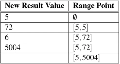
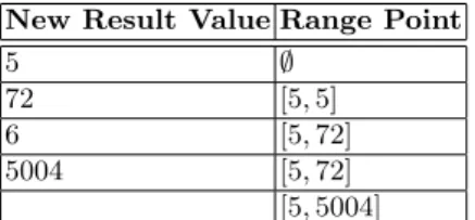
Dynamic Range screeners use segments that contain all valid values recorded during the training phase to determine if a variable is within its expected behavior. The number of segments created is variable and each segment represents a range of values that the invariant considers valid. On Table2.2and Table2.3, it is possible to see how the ranges are updated when a new value occurs during the training phase.

Table 2.2: Dynamic Range Screener training with one segment New Result Value Range Point

5 /0

72 [5,5]

6 [5,72]

5004 [5,72]

[5,5004]

When only one segment is used, its bounds are updating according to the following expres-sions:

State of the Art

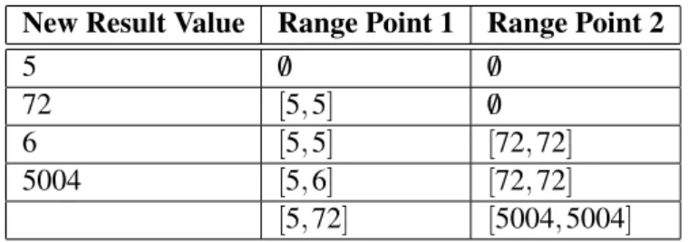
Table 2.3: Dynamic Range Screener training with two segments New Result Value Range Point 1 Range Point 2

5 /0 /0 72 [5,5] /0 6 [5,5] [72,72] 5004 [5,6] [72,72] [5,72] [5004,5004] l : = min(l,v) (2.1) u : = max(u,v) (2.2)

where l is the lower bound, u is the upper bound and v is the value observed from the variable. In other words, when the observed value is out of bounds of the current range, the segment is extended to include the new value [AGZvG08b].

With more segments, the process of updating the boundaries is a little different. If the new value is not contemplated withing the boundaries of any of the segments, an update will be made. This update will rearrange the segments in a way that the segments allows the smallest possible set of values, maintaining all the valid values from the previous iteration.

In the error detection phase, the value of a variable is compared with the ranges accepted by the fault screener. The following expression is used to evaluate if the variable is showing a perturbation:

violation = ¬(l < v < u) (2.3) where l is the lower bound, u is the upper bound and v is the value observed from the vari-able. When more then one segment exists, the variable must be within one of the ranges to be valid [AGZvG08b].

The main advantage of this type of fault screeners is its ability to represent a large set of valid values for a variable. However, it suffers from increasing this value set to quickly when adding values that are distant from the current ranges or when two ranges are merged.

2.2.3.3 Invariance-based Screener

This type of fault screener stores two fields: the first observed value and a bitmask representing the bits that were altered. In other words if the first observed value was 2 (represented by 0010) and the next observed value was 3 (represented by 0011), then the value 2 would be saved along with the bitmask 0001, because only the last bit was altered between the two values.

State of the Art

During the training phase, the bitmask is updated to accommodate all the changes that were made to the first value, in a bitwise fashion. The following expression is used to update the bitmask:

msk = ¬(new ⊕ f st) ∧ msk (2.4)

where msk is the bitmask, new is the currently observed value and f st is the first observed value. Both the xor and the and operators are bitwise operators [AGZvG08a].

To validate the value of a variable during the error detection phase, another expression is used:

violation = (new ⊕ f st) ∧ msk (2.5)

where msk is the bitmask, new is the currently observed value and f st is the first observed value. Again both operators are bitwise. When violation is not zero, a perturbation is de-tected [AGZvG08a].

Invariance-based screeners have a very efficient representing the valid value set, but is limited in its representation of negative and floating point values. It is also possible to render the screener useless with only two instructions if the values differ on all their bits [RCMM07].

2.2.3.4 TLB-based Screener

The TLB-based screener has its basis on TLB memory access hits and misses. TLB misses are regarded as perturbations and accesses that don’t cause a miss are regarded as normal.

This screener is mostly used to locate errors on data-addresses, although it cannot find per-turbations when these are present on the low-order bits of the address. It can only find faults that affect the data-addresses [RCMM07].

2.2.3.5 Bloom Filter Screener

This type of screener uses data structures called Bloom filters to maintain the entire set of values that a variable had during the training phase. A 32-bit value that merges the observed value and the instruction address is used to store the accepted values. This 32-bit number is defined as follows:

g = (v ∗ 216)∨ (0xFFFF ∧ ia) (2.6)

where v is the observed value and ia is the instruction address. The operators ∨ and ∧ are bitwise operators [AGZvG08b].

During training, when a new value observed, the number g is hashed on two different functions (h1and h2). The hash functions are updated according to the following expressions:

State of the Art

b[h1(g)] : = 1 (2.7)

b[h2(g)] : = 1 (2.8)

where h1and h2are hash functions [AGZvG08b].

After the training phase, to detect errors the following expression is used:

violation = ¬(b[h1(g)] ∧ b[h2(g)]) (2.9)

where h1and h2are hash functions.

The main advantage of this type of screener is the maintaining of the full history that the variable had during the training phase.

2.2.4 Fault Screener Evaluation Metrics

In order to evaluate the performance of fault screeners, three different metrics are used. The first of these metrics is fault coverage. This is measured by counting the number of injected errors that were found. The higher the number of errors detected, the greater the coverage is.

The second metric is the accuracy of the fault screener. This metric is measured by the quantity of false positives, errors detected that do not exist, encountered during successful executions of a program. Less false positives means better accuracy.

The last metric is latency, which is the distance the actual error and where it is detected. These metrics cannot be taken into account separately. For example a fault screener could have a very high performance if an error is detected on every line, however if the majority of those errors don’t exist, those would represent false positives, in other words, the fault screener would have a very low accuracy [RCMM07,AGZvG08a].

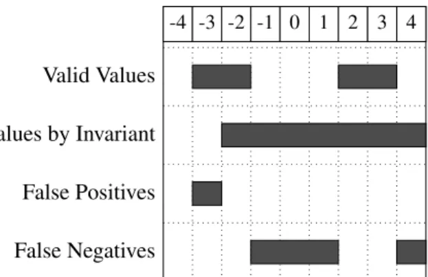
One of the challenges for using generic invariants is the accuracy of the error detection, as with the increase of executions used for training, the rates of false positives and false negatives differ. The number of false positives tends to decrease, while the number of false negatives, the non detection of existing errors, increases [AGZvG08b]. This happens because of the increase of accepted values by the invariant.

Figure2.2displays a possible setup for a dynamic range invariant. During the training phase the invariant learnt that the values between −2 and 2 were the valid set of possible values. However the real case is that the values should be valid between −3 and −1, as well as 1 and 3. This leads to some false positives and false negatives. Values observed that withing the ranges [−3,−2[ or ]2,3] issue a detected error warning, hence they are false positives. Likewise, observations between −1 and 1 do not issue any warnings when they should.

In the same scenario, if the invariant had been subject to more training, then more values would be added into the accepted range. On Fig.2.3 the number 4 was such a value. This lead to the

State of the Art

-4 -3 -2 -1 0 1 2 3 4

Valid Values Accepted Values by Invariant False Positives False Negatives

Figure 2.2: False positive and false negative example

values ranging from 2 to 3 to become valid, eliminating those false positives, but the ones from 3 to 4 also became valid, becoming new false negatives. In other words, there was an increase of false negatives and decrease of false positives. With more training the false positive rate tends to lead to 0 because the entire possibility of values become valid.

On the other side, the number of false negatives increases because since it accepts a lot more values then it should, it does not detect any values outside the huge accepted range.

-4 -3 -2 -1 0 1 2 3 4

Valid Values Accepted Values by Invariant False Positives False Negatives

Figure 2.3: False positive and false negative example with increased training

2.2.5 Quality Comparison

In order to compare the different types of screeners, Paul Racunas et al. made a study where these fault screeners were used on several benchmarking suites [RCMM07].

As it can be seen in the study’s results, each type of fault screener behaves differently on the various benchmarks. This is due to the very nature of the screener. Some are more susceptible to destructive aliasing (i.e. the invariance screener). However, on a more global note, the results are positive showing a fairly high coverage and very low false positive rates, apart from the TLB-based screener that shows a much larger false positive rate.

State of the Art

2.2.6 Tools

There are already applications that generate invariants to monitor the execution of a program. Among these applications is the toolset called Zoltar [JAvG09]. This application applies a fault screener on every occurrence of a variable and tries to detect errors by finding perturbations on their behavior. In addition to detecting errors, Zoltar uses the errors detected to help debugging using SFL. No type of variable selection optimization is present, which makes its use to slow on larger applications.

Another tool that works with fault screeners is PRECIS [SAKV11]. PRECIS uses a different type of invariants based on pre- and post-conditions. However, this application doesn’t offer any other kind of feature.

DIDUCE [HL02] is yet another application that uses fault screeners. This tool does not gen-erate invariants automatically, it is the user who must decide where he wants code to be analyzed. It is used to help debugging Java implemented applications.

Daikon [EPG+_{07] is a tool that reports likely invariants. It runs a program and then reports}

the properties observed during the executions. Besides storing pre-defined invariants like con-stants, range or linear relationships, it can be extended by the user with new invariant types. It is compatible with various programming languages, includingC,C++,JavaandPearl.

Carrot [PRKR03] is a tool created with the purpose of using generic invariants for fault lo-calization. It uses a smaller set of invariants then Daikon. The results obtained were negative which lead to the belief that invariants alone are insuficient as a means of debugging. However, in [AGZvG08b] the use of invariants for fault localization was successful when used as the input for the fault localization technique SFL.

IODINE [HCNC05] is a framework for extracting dynamic invariants for hardware designs. It has been shown that accurate properties can be obtained from using dynamic invariants.

iSWAT[SLR+08] is another framework that uses invariants for error detection of a hardware

level. It usesLLVMto instrument the source code to monitor the store values.

2.3 Collar Variables

Collar Variables is a term used to describe the key variables of a system. According to Tim Menzies et al. [MOR07] it is curious how software works as even an application with only 300 variables can generate up to 2300 _{states. This could be because only a sub-set of variables are}

responsible for the output of the system and, as such, only those variables need to be monitored to have control of the system [MOR07].

So if these collar variables are the true of the behavior of software, three things are to be expected:

• Quick saturation of software testing due to the early execution of all program paths. • Random mutation testing most probably won’t change the behavior of the program, as it is

State of the Art

• Clumping of reachable states due to the settings that the collar variables allow [Pel04].

2.3.1 Tools

There are already some tools that try to approach the concept of collar variables. One of these tools isTAR3, a randomized version of the data-miner TAR2 [MH03]. This tool tries to find the collar

variables of an application by creating different scenarios that allow their identification. There is also an updated version calledTAR4.1.

In [GMDGB10] the algorithms ofTAR3andTAR4.1are explained. These algorithms allow

to obtain a ranking of “usefulness” of the different components of an application. TAR3uses the

concepts of lift, the change that a decision makes on a set of examples, and support.TAR4.1uses

Naive Bayes classifiers for the scoring heuristic in order to obtain an overall better performance in comparison toTAR3.1.

KEYS[JMF08] is yet another algorithm that tries to discover the collar variables, called keys

by the author. It is used to optimize requirement decisions and is faster then theTAR3algorithm.

In [GMJ+_{08], an improved KEYSalgorithm is shown calledKEYS2. It outperforms the original}

version by four orders of magnitude in terms of speed.

The main problem with these approaches is the need to execute the application various times to obtain the collar variables.

In [WGS03], the concept of collar variable is once again used, this time by the name of back doors. They were using these back doors to solve CSP/SAT search problems and suggest by formal analisys the potencial improvement of some hard problems from an exponential to polynomial time.

Chapter 3

Implementation Details

In this chapter, some insight on the implementation details of the approached solution is given. It is divided into four main sections. First a section describing the changes made to the GZoltar toolset in terms of instrumentation. After that, the invariant structure used is presented and the following section explains how this invariant management works. Lastly, the variable evolution pattern detectors are presented.

This was necessary in order to achieve the thesis goals. To add automatic error detection with invariants, changes to the instrumentation had to be made to make the target program call the update and validate functions of the invariant. Likewise, the pattern detectors were necessary to discover variables that are not important to monitor.

As GZoltar is a plug-in for the Eclipse IDE and it works withJavaapplications, these changes

had to follow the same requirements.

3.1 Instrumentation

The GZoltar toolset already used some degree of instrumentation in order to evaluate the code coverage of the executed tests. However major changes were needed in order to monitor variables. All the changes to the instrumentation were made using theASM4.0framework. Due to the way Java variables work, during the execution there is no information regarding the name of the

variables being used, only their stack index. This lead to the first change needed. In order to have this information, an analysis of the local variable table is required. This table provides data on the variables including: variable name, the stack index used and the instructions ehen the variable is associated to the index. During the analysis, when a new variable is encountered during the training phase, an invariant is created. If the invariant already exists, then the stack index and the offset of instructions when the variable is used are updated.

Having the invariants created, to one thing that is missing is alter the execution to call the invariant’s update and validate function. This is accomplished by invoking the invariant manager’s

Implementation Details

update function, when in training mode, or the valitade function in error detection mode (for more details on these functions check Section3.3).

3.2 Invariant Structure

Since GZoltar does not have any invariant support, a new data structure had to be devised to maintain the information relevant the invariant, like learnt information and functions for training and validation. It also had to incorporate the functions to detect variable patterns (explained in Section3.4) and save the pattern information.

Since there are various types of invariants and restraining the implementation to a single type is not ideal, a hierarchical approach was used. There is a global abstract class calledInvariant

that imposes the data that is common to every invariant type. It also implements functions that are shared by every invariant as well, like the Variable Evolution Pattern Detectors.

Each type of invariant is a subclass of Invariant that implements the functions that,

al-though are common to every invariant, are implemented differently. It also adds variables that are specific to said invariant. Both dynamic range invariants and bitmask invariants were imple-mented.

These are the variables that are used by every invariant type and as such are present in class

Invariant:

• className– The class that the variable monitored by invariant belongs to.

• method– The method that the variable monitored by invariant belongs to.

• name– The name of the variable monitored by invariant.

• index– The stack index used by the variable during the execution.

• start– The instruction number of when the variable starts using the designated index.

• end– The instruction number of when the variable stops using the designated index.

• typeDescriptor– The type descriptor of the variable.

• nRuns– Number of executions where the variable is used (pattern detection).

• firstValue – A boolean indicating if the variable has been used before in the current

execution (pattern detection).

• delta– The difference between the last two observed values (pattern detection).

• lastValue– The last observed value during the current execution (pattern detection).

• deltaPattern– Information if the delta pattern was broken (pattern detection).

• lowerBoundRun– Lowest observed value of the current execution, or of the last execution

(pattern detection).

Implementation Details

• upperBoundRun– Highest observed value of the current execution, or of the last execution

(pattern detection).

• rangePattern– Information if the range pattern was broken (pattern detection).

• nVisits– Number of times the invariant was used (pattern detection).

There are also various functions that are common to all invariants. The functions that are used for pattern detection have the same implementation, however there are other that may need implementation within the subclass. The functions ofInvariantare:

• boolean withinOffset(int offset) – Determines if the offset given allows the

invariant to be used.

• void updateCollarStatus(Object value)– Updates the pattern detection

info-mation with a new value.

• boolean hasPattern()– Indicates if a pattern exists or not.

• void update(Object value)– Updates the information learnt with a new value

(re-quires subclass implementation).

• boolean validate(Object value) – Checks if the value follows the valid

para-maters set by the invariant (requires subclass implementation).

• String invariantToString()– Turns the invariant into a string that is used to save

the invariant (requires subclass implementation).

With this implementation, extension to new invariant types is very accessible, one of the main goals when this structure was conceived.

3.3 Invariant Management

In addition to the instrumentation and invariant structure, an invariant management system was required. To accomplish this, the classLoadStoreMaintainerwas created. This class contains

a table that is used to maintain the invariants during the execution. It also implements the save and load functions of the invariants. There are two load modes, a complete mode that loads all invariants (used for the training phase) and a collar load mode that only loads the invariants that did not detect patterns (for error detection mode).

LoadStoreMaintaineralso contains an update and a validate function that find what

in-variant that needs to be used, by knowing its stack index and instruction offset, and calls the invariant’s own update or validate.

Implementation Details

3.4 Variable Evolution Pattern Detectors

In order to know what variables need to be monitored and which can be discarted, two diferent de-tectors were created. Each detector tries to enconter its own pattern on the evolution of a variable’s value. When the detector sees that the pattern is broken, then the variable is marked as important to be monitored.

These patterns were designed to be as simple as possible, while still detecting constants and other variables, like counters. It is important to note that a variable is never classified as not important to monitor if it was only used on one execution of the system.

3.4.1 Delta Oriented Pattern Detector

The Delta Oriented Pattern Detector is the first of two algorithms created to detect collar variables. With this detector, the main objective is to discover variables that throughout its life cycle evolve in a constant fashion. These variables are then deemed not essencial since during every execution its value increases or decreases in the same manner, no matter what the input is. This is accomplished by using a delta value (∆), that is the difference between the last value observed and the current one:

∆:= current value − last value if last value 6= /0 (3.1) ∆:= 0 if last value = /0 (3.2) Algorithm1demonstrates how this detector can determine which variables are important to monitor. Every variable in the system has a ∆ associated to it. During the training phase, when the first value is observed, ∆ is given the value 0 and the last value is updated to the observed one. On the next observation, ∆ will be updated accordingly, using the current value and the last value, as seen in Line 9. After this, the pattern detection begins. With each observation, an updated ∆ is generated (∆2) and is compared to the current ∆. If the new ∆ is equal to the current one,

the pattern detection continues as the evolution of the variable remains the same. In case the ∆ is different, since the pattern is broken, a flag is stored indicating that this pattern does not exist for the variable being evaluated. There is, however, an exception to this. When the new ∆ is 0, then it is not compared to the previous ∆ (Lines13and24). This is done because variables can be accessed without their values being changed.

After each execution, the value of ∆ is saved along with a flag indicating whether the pattern was broken or not. Subsequent executions use the ∆ from the first execution and starts the pattern detection after the first two values, instead of after the third like the first run.

With this detector it is possible to detect constant values (∆ = 0), as well as counters and loop variables that always increment/decrement with the same pace. A good example of this is the

Javacode present on Listing3.1. Of all the variables from this small code sample,jis the one

that has the least impact on the outcome. It only serves as an auxiliary variable for the loop. 16

Implementation Details

Algorithm 1 Delta Oriented Pattern Detector

1: pattern := true 2: for all Execution do 3: for all Observation do 4: if nRuns = 0 then

5: if first observation then 6: ∆:= 0

7: LastValue := ObservedValue 8: else if second observation then 9: ∆:= ObservedValue − LastValue 10: else 11: ∆2:= ObservedValue − LastValue 12: LastValue := ObservedValue 13: if ∆ 6= ∆2V∆26= 0 then 14: pattern := f alse 15: end if 16: end if 17: else

18: if first observation then 19: ∆:= 0 20: LastValue := ObservedValue 21: else 22: ∆2:= ObservedValue − LastValue 23: LastValue := ObservedValue 24: if ∆ 6= ∆2V∆26= 0 then 25: pattern := f alse 26: end if 27: end if 28: end if 29: end for 30: nRuns + + 31: end for

The delta oriented pattern detector can be used to mark this variable as not essencial. It does not matter what the input of this function is, becausejwill always increment in the same manner.

∆will always be 1 (jalways starts with the value 0 and increments by one on every access), so

the pattern is never broken.

3.4.2 Range Oriented Pattern Detector

One of the main differences between this pattern and the previous one is that the range oriented pattern detector requires one full execution before it can determine a broken pattern. The basis of this detector is that if the range of values that a variable has between every run is the same, then it is not important to monitor. This is what happens on Listing3.2where in every execution j has values with the range [0,5]. This is the reason why one full execution is required. The detector only has the range of the full execution at the end of it.

Implementation Details

1 public int funcExample(int i) { 2 int accumulator = i; 3 for(int j = 0; j < 3; j++) { 4 if(accumulator == 1) 5 break; 6 _{accumulator *= accumulator;} 7 }

8 int result = accumulator * 3;

9 return result;

10 }

Listing 3.1: Delta Detector code example

The functions of updating the bounds of the range are the same as the dynamic range invariant:

l := min(l,v) (3.3)

u := max(u,v) (3.4)

The main difference between the dynamic range invariant and the range oriented pattern detec-tor is that the bounds of the detecdetec-tor are only updated on the first execution that a variable appears in. On the following executions, every time a new value is observed, it is determined if it is within the range of the first execution:

broken = ¬(l < v < u) (3.5)

Algorithm 2shows how the detector works. During the first execution (Lines 4 and5) the range is constantly updated with every observation of a given variable. Once the first execution is over, the pattern detector is ready to discover a pattern. Hence, on the following executions, each observed value is compared to the pattern detector range, as seen in Line7. If the new value is not within the range determined by the first execution, then the pattern was broken. If this never happens then it is determined that there is a pattern in the execution and the variable will not be monitored during the error detection phase.

With this detector it is possible to detect variables that although do not evolve in a linear way that can be detected by the delta oriented pattern detector, are restricted in some way during the execution. This is the case of loop variables that are affected within the cycle. This can be seen in the example shown on the example shown on Listing 3.2. In this case, variable j is not a

very important variable to be monitored. Taking into account the previous, detector, it is easy to understand that it would not be marked as not essencial (as ∆ can be both 1 or 2). However the range oriented detector can find a pattern. On every execution, despite what input is received, the range of values jtakes is always [0,5]. During the first execution, this range would be given to

Implementation Details

Algorithm 2 Range Oriented Pattern Detector

1: pattern := true 2: for all Execution do 3: for all Observation do 4: if nRuns = 0 then

5: updatePatternRange(ObservedValue)

6: else

7: if ObservedValue /∈ PatternRange then 8: pattern := f alse 9: end if 10: end if 11: end for 12: nRuns + + 13: end for

the pattern detector and the following runs would follow the pattern, so the variable would not be monitored.

1 public int funcExample(int i) { 2 int accumulator = i; 3 for(int j = 0; j < 5; j++) { 4 if(accumulator == 1 && j < 3) 5 j=j+2; 6 accumulator *= accumulator; 7 }

8 int result = accumulator * 3;

9 return result;

10 }

Implementation Details

Chapter 4

Empirical Results

In this section the experimental setup is presented, along with the workflow of the experiments themselves. After that the experimental results are discussed.

4.1 Experimental Setup

During the experimentation, three real world applications were used: • NanoXML1- a XML parser.

• org.jacoco.report2- a report generator for theJaCoColibrary.

• XML-Security- a XML signature and encryption library from the Apache Santuario 3

project.

On Table4.1some details of the applications used are shown. These details include the number of lines of code and the number of test cases.

Table 4.1: Application details

Subject LOC Test Cases

NanoXML 5393 9 org.jacoco.report 5979 235

XML-Security 60946 462

NanoXMLis a free, easy to use and non-GUI based and non-validating XML parser for Java.

It has three different components:

• NanoXML/Java, the main standard parser.

1_{NanoXML –http://devkix.com/nanoxml.php}

2_{JaCoCo –http://www.eclemma.org/jacoco/index.html} 3_{Apache Santuario –http://santuario.apache.org/}

Empirical Results

• NanoXML/SAX, anSAXadapter for the standard parser.

• NanoXML/Lite, an extremely small version of the parser with limited funcionality. NanoXMLis available under the zlib/libpng license, which is Open Source compliant.

JaCoCois an open source code coverage library for Java, being developed by EclEmma. The

current goal of JaCoCo is to provide a code coverage library that is able to provide coverage

reports. To do this there is a bundle calledorg.jacoco.report. This bundle is able to provide

reports in three formats: • HTML, for end users.

• XML, to be processed by external tools.

• CSV, suitable for graph creation.

XML-Securityis one of the libraries available on the Apache Santuario project, a project

that aims at providing security standards for XML. It is distributed under the Apache Licence Version 2.0 which is compatible with other open source licenses. The XMLSecurity data format provides encryption and decryption XML payloads at different levels, namely Document, Ele-ment and EleEle-ment Content. XPath can be used for multi-node encryption/decryption. There exist two versions of XML-Security: a Java one and a C++ one. The Java version is used for the

experiments.

4.1.2 Workflow of Experiments.

In order to determine if the pattern detectors were effective at reducing the number of instrumented points and if the error detection maintained a good quality, the system’s variables is subject to training first. Each application is instrumented in order to train the fault screeners. This training is achieved by executing a random number of test case (roughly 50% of the tests in the original suite) of the target program. We did not use the complete suite in order not to influence the results positively.

Once the training of the fault screeners is complete, the error detection phase begins. To eval-uate the quality of the error detection, each application is executed five times. On each execution a different bug is inserted into the code and the number of false positives and false negatives are col-lected. An additional execution is performed without any inserted bug to determine the execution time in a regular scenario. Each application’s test suite was executed without any instrumentation as well to determine the increase of time the instrumentation brings.

Figure4.1shows how each phase behaves during the experiment. Before the training phase, when the application is compiling, the code is instrumented using theASM4.0framework. Once

instrumented, the altered application can be used on the next phase. During this next phase, the training phase, the test are executed with the instrumented code. Everytime a variable is used, the update function of the screener is called in order to update the accepted values. In addition,

Empirical Results

the screener uses the pattern detectors to detect broken patterns. At the end of the execution, both the invariant and the data collected from the detector are saved. On the operational phase the test cases are executed with the instrumented code once again. However, this time instead of monitoring every variable, only the variables that did not have a detected pattern are observed. On each observation the value is then evaluated by the screener with the information gathered during the training.

.jar

Screener

Pattern

Detectors

.jar

Screener

Error Detection Result Operational Phase

.jar

libscreener

Compiling Phase

.java

.class

Empirical Results

Injected bugs are of different types to guarantee a more varied input. Some examples of inserted bugs are:

• Change an operator when assigning values (i.e. change + to −). • Change a random numeric value.

• Change comparation operator of a conditional clause (i.e. change a > to < on anifclause).

• Change the value of an argument of a function call.

These bugs where inserted on random parts of each program, with the only caution being affecting a numerical value since implemented invariants are unable to monitor non numerical values. With this setup the expected results are:

• Value of the reduction obtained in the number of used invariants.

• Comparison of execution times between executions with and without instrumentation. • Accuracy of the error detection with the use of pattern detectors.

4.2 Results

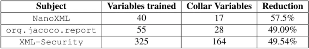
Table 4.2 shows the number of variables that were trained and the number of variables that are considered collar variables by the pattern detectors. It is important to note that only numerical variables are subjected to training, in other words, only variables of the typesint,long,double

andfloat.

Table 4.2: Variable reduction

Subject Variables trained Collar Variables Reduction

NanoXML 40 17 57.5% org.jacoco.report 55 28 49.09%

XML-Security 325 164 49.54%

On average, a reduction of 52.04% is achieved with the use of the two pattern detectors. However the execution time of the program with instrumentation is also important to take into consideration. Table 4.3 presents the execution times of the test suites both with and without instrumentation.

The average increase in the execution time is 135.8%. Although this seems like a high value, it is greatly impacted by the increase noticed onNanoXMLthat is only a few miliseconds.

Having the data on the reduction of variables monitored and execution time increase, the qual-ity of the error detection is what remains. To test the qualqual-ity of the detection using these collar variabes, the number of false positives (Nf p) and false negatives (Nf n) was determined. Recall that

a false positive is considered when the fault screener detects an error in the execution that does not 24

Empirical Results

Table 4.3: Execution time increase

Subject _{instrumentation (ms)}Execution time with Execution time without Increase_{instrumentation (ms)}

NanoXML 270 827 206.3% org.jacoco.report 3469 5162 48.8%

XML-Security 25005 63088 152.3%

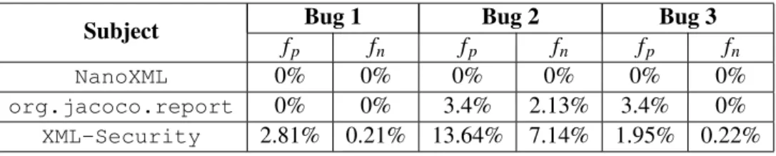
Table 4.4: False positive ( fp) and false negative rate ( fn) for bugs 1, 2 and 3

Subject _f Bug 1 Bug 2 Bug 3

p fn fp fn fp fn

NanoXML 0% 0% 0% 0% 0% 0% org.jacoco.report 0% 0% 3.4% 2.13% 3.4% 0% XML-Security 2.81% 0.21% 13.64% 7.14% 1.95% 0.22%

Table 4.5: False positive ( fp) and false negative rate ( fn) for bugs 4 and 5

Subject _f Bug 4 Bug 5

p fn fp fn

NanoXML 0% 66.67% 0% 0% org.jacoco.report 3.83% 2.13% 5.96% 0% XML-Security 12.99% 0.22% 0.22% 0.22%

exist. Likewise, a false negative is counted when a faulty execution has no objections raised from any fault screener.

The results shown on Tables4.4and4.5were obtained by comparing the total number of false positives (Nf p) and false negatives (Nf n) with the number of tests on the test suite of the target

program (Nt).

fp:= Nf p

Nt (4.1)

fn:= Nf n

Nt (4.2)

With an average of 3.21% rate of false positives and 5.26% rate of false negatives, the rate of these false results is considerably low, especially on the smaller applications. On the largest ap-plication,XML-Security, although having a higher rate of false results, the worst case scenario

detected was a 13.64% fpand 7.14% fn.

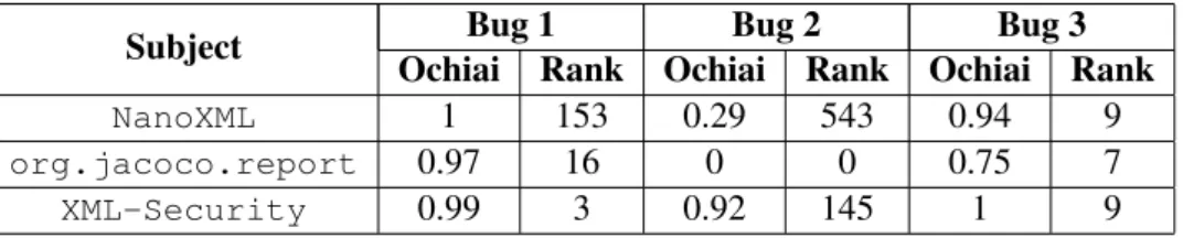
Lastly, in order to determine how well these collar variables can be used on Spectrum-based Fault Localization, the Ochiai coeficient obtained on each bug inserted is shown on Tables4.6and

4.7for the runs with no instrumentation and on Tables4.8and 4.9for the runs with instrumenta-tion. The number of lines required to inspect in order to find the bug is also present. This number actually represents the ranking that the bug had on the list with the Ochiai of every element. It can be noted that excluding very few cases, the required amount of lines that a programmer needs to

Empirical Results

inspect and the Ochiai coeficient, the SFL similarity coefient used on GZoltar, obtained are very similar when using the solution with invariants when compared with the one without invariants.

Table 4.6: Ochiai results for bugs 1, 2 and 3 without instrumentation Subject _{Ochiai Rank Ochiai Rank Ochiai Rank}Bug 1 Bug 2 Bug 3

NanoXML 1 153 0.29 543 0.94 9 org.jacoco.report 0.97 16 0.71 3 0.71 3 XML-Security 0.83 3 0.84 35 0.89 9

Table 4.7: Ochiai results for bugs 4 and 5 without instrumentation Subject _{Ochiai Rank Ochiai Rank}Bug 4 Bug 5

NanoXML 0.93 53 0.47 243 org.jacoco.report 0.75 1 0.58 10

XML-Security 0.83 5 0.93 3

Table 4.8: Ochiai results for bugs 1, 2 and 3 with instrumentation Subject _{Ochiai Rank Ochiai Rank Ochiai Rank}Bug 1 Bug 2 Bug 3

NanoXML 1 153 0.29 543 0.94 9 org.jacoco.report 0.97 16 0 0 0.75 7 XML-Security 0.99 3 0.92 145 1 9

Table 4.9: Ochiai results for bugs 4 and 5 with instrumentation Subject _{Ochiai Rank Ochiai Rank}Bug 4 Bug 5

NanoXML 0.27 1634 0.47 243 org.jacoco.report 0.11 491 0.73 19

XML-Security 1 5 1 3

In conclusion, with only the use of two pattern detectors, the decrease of used invariants is quite significant and the error detection quality remains very high, appart from some special cases. The quality of the fault localization does not seem to be affected a lot (save for some exceptions). However, in terms of execution time, the obtained results may still not be enough to allow their use on real world markets, but perhaps the creation of even more detectors could be a solution.

4.3 Threats to Validity

The main threat to the validity of these results is the fact that only three test subjects were used during the experimentation. Despite these subjects being real world applications being diverse in

Empirical Results

both the size of the application (lines of code) and size of the test suite, the limited number of sub-jects implies that not all types of system’s are tested. This means that a system with characteristics that are completly different might present different results. Another threat is that the number of injected bugs is not enough to lead to accurate results, as these bugs might simply be “lucky bugs” that intercept a collar variable.

Naturally, there are also threats that are based on the implementation of the invariants, the instrumentation or the pattern detector algorithms themselves. The reduce these threats, additional testing was made prior to the experimentation to guarantee the quality of the experimental results in this regard.

Empirical Results

Chapter 5

Conclusions and Future Work

5.1 Conclusions

In sum, although there are already attempts at automating debugging with the use of fault screen-ers, it is still not effective due to the large overhead of the current solution, monitoring every variable on the system. The use of the concept of collar variables could prove invaluable to solv-ing this problem, as by ussolv-ing fault screeners only on collar variables would enable a much lighter execution of the applications. However, current collar variable detection algorithms at the moment require multiple executions, which is not the ideal situation when the objective is to be integrated in the testing phase.

5.1.2 Empirical Results

In this paper two simple detectors were used to evaluate what were the collar variables of each of the systems. Experimenting on real world applications led to a more accurate take on the impact of the use of invariants for error detection. By only using two detectors, the reduction of number of invariants used was above 50% while still maintaining good quality detection. Still the increase in execution time might still be too severe for use and the inability of the detectors to view patterns on non numeric values is still an obstacle.

These results were submitted in a paper for ICTSS’12. The publication is available on Ap-pendixA.

5.2 Future Work

For future work in order to reduce the overhead, a further decrease in the number of invariants used is necessary. The study of additional detectors that would filter even more variables. Another option is the use of an algorithm similar to the one used on TAR4.1 [GMDGB10] to make the decision of what variables to monitor.

Conclusions and Future Work

Futher work will also be invested in tackling one of the main issues of the current approach, the ability to only evaluate numeric variables. Efforts will be made to use invariants and create de-tectors that would evaluate patterns for other variable types likeStringorchar. These variables

may prove invaluable to increasing the effectiveness of this method. With a proper algorithm for convertingStringtoint, it would be possible to use current invariants and produce detectors

for these data types easier.

By investing work into this area, high error detection rates could be achieved and the impact on performance greatly reduced paving the way for self-healing systems.

References

[AGZvG08a] Rui Abreu, Alberto González, Peter Zoeteweij, and Arjan J.C. van Gemund. Auto-matic software fault localization using generic program invariants. In Proceedings of SAC’08, pages 712–717, 2008.

[AGZvG08b] Rui Abreu, Alberto González, Peter Zoeteweij, and Arjan J.C. van Gemund. On the performance of fault screeners in software development and deployment. In Proceedings of ENASE’08, pages 123–130, 2008.

[AZvG07] Rui Abreu, Peter Zoeteweij, and Arjan J.C. van Gemund. On the accuracy of spectrum-based fault localization. In In Proceedings of TAIC’07, pages 89–98. IEEE, 2007.

[DZ09] Martin Dimitrov and Huiyang Zhou. Anomaly-Based Bug Prediction, Isolation, and Validation: An Automated Approach for Software Debugging. In In Proceed-ings of ASPLOS’09, volume 44, pages 61–72. ACM, 2009.

[ECGN99] Michael D. Ernst, Jake Cockrell, William G. Griswoldt, and David Notkin. Dy-namically Discovering Likely Program to Support Program Evolution Invariants. In Proceedings of ICSE’99, pages 213–224, 1999.

[EPG+_{07] Michael D. Ernst, Jeff H. Perkins, Philip J. Guo, Stephen McCamant, Carlos}

Pacheco, Matthew S. Tschantz, and Chen Xiao. The Daikon system for dynamic detection of likely invariants. Science of Computer Programming, 69(1-3):35–45, December 2007.

[GMDGB10] Gregory Gay, Tim Menzies, Misty Davies, and Karen Gundy-Burlet. Automatically finding the control variables for complex system behavior. Automated Software Engineering, 17(4):439–468, May 2010.

[GMJ+_{08] Gregory Gay, Tim Menzies, Omid Jalali, Martin Feather, and James Kiper.}

Real-time Optimization of Requirements Models. Jet Propulsion, pages 1–33, 2008. [HCNC05] Sudheendra Hangal, Naveen Chandra, Sridhar Narayanan, and Sandeep

Chakra-vorty. IODINE : A Tool to Automatically Infer Dynamic Invariants for Hardware Designs. In Proceedings of DAC’05, pages 775–778, 2005.

[HL02] Sudheendra Hangal and Monica S. Lam. Tracking down software bugs using auto-matic anomaly detection. In proceedings of ICSE’02, pages 291–301, 2002. [JAvG09] Tom Janssen, Rui Abreu, and Arjan J.C. van Gemund. Zoltar: a spectrum-based

REFERENCES

[JH05] James A Jones and Mary Jean Harrold. Empirical Evaluation of the Tarantula Au-tomatic Fault-Localization Technique Categories and Subject Descriptors. In Pro-ceedings of ASE’05, pages 273–282, 2005.

[JMF08] Omid Jalali, Tim Menzies, and Martin Feather. Optimizing Requirements Deci-sions with KEYS. In proceedings of PROMISE’08 (ICSE), pages 1–8, 2008. [MH03] Tim Menzies and Ying Hu. Data Mining for Very Busy People. Computer, pages

22–29, 2003.

[MJ96] Christoph C Michael and Ryan C Jones. On the Uniformity of Error Propagation in Software. In Proceedings of COMPASS’97, (70), 1996.

[MOR07] Tim Menzies, David Owen, and J. Richardson. The strangest thing about software. Computer, 40(1):54–60, 2007.

[Pel04] Radek Pelánek. Typical structural properties of state spaces. In Proceedings of SPIN’04 Workshop, (201):5–22, 2004.

[PRKR03] Brock Pytlik, Manos Renieris, Shriram Krishnamurthi, and Steven P Reiss. Au-tomated Fault Localization Using Potential Invariants. In Proceedings of AADE-BUG’03, pages 273–276, 2003.

[RAR11] André Riboira, Rui Abreu, and Rui Rodrigues. An OpenGL-based eclipse plug-in for visual debugging. In Proceedings of TOBI’11, pages 5–8, 2011.

[RCMM07] Paul Racunas, Kypros Constantinides, Srilatha Manne, and Shubhendu S Mukher-jee. Perturbation-based Fault Screening. In Proceedings of HPCA’07, pages 169— -180, 2007.

[SAKV11] Parth Sagdeo, Viraj Athavale, Sumant Kowshik, and Shobha Vasudevan. PRE-CIS: Inferring invariants using program path guided clustering. In Proceedings of ASE’11, pages 532–535, 2011.

[SLR+_{08] Swarup Kumar Sahoo, Man-Lap Li, Pradeep Ramachandran, Sarita V. Adve,}

Vikram S. Adve, and Yuanyuan Zhou. Using likely program invariants to detect hardware errors. In Proceedings of DSN’08, (June):70–79, 2008.

[Tas02] Gregory Tassey. The economic impacts of inadequate infrastructure for software testing. National Institute of Standards and Technology RTI Project, 2002.

[WGS03] Ryan Williams, Carla P Gomes, and Bart Selman. Backdoors To Typical Case Complexity. In Proceedings of IJCAI’03, 2003.

Appendix A

Lightweight Approach to Automatic Error Detection

Using Program Invariants

J. Santos1_{, R. Abreu}1

1_{Department of Informatics Engineering, Faculty of Engineering, University of Porto, Portugal.} Despite all efforts made during the development phase to test the application thoroughly, errors always creep to the operational phase. To fix these errors, a debugging phase is required, where the faults are located and fixed. This, however, is a costly process [1] and locating faults can be a very difficult task. Automating the process of locating the root cause of observed failures is one of the possible ways to reduce the cost of debbuging. In order to address this issue, tools like Zoltar [2] were developed. Through the use of generic invariants, also known as screeners, it is possible to predict the location of a faulty code segment, using Spectrum-based Fault Localization [3]. These fault screeners are software constructs that detect errors on the values of variables [4].

However this method presents some obstacles to its use on real applications. Using a fault screener on all occurences of every variable creates an immense overhead. To reduce this overhead, it is necessary to decrease the number of instrumented points on the code. To achieve this, a possible solution would be to discover what are the collar variables of the system and only monitor those variables. According to Tim Menzies [5], collar variables are the key variables of the system that truly influence its behavior.

Another situation faced when using screeners is the accuracy of the results given by the screeners. Fault screeners are prone to produce erroneous results. These results can either be false positives, when an unexistant error is detected, or false negatives, when no error is detected in the presence of one. This happens because of the training screeners must go through during testing of the development phase. Since each passed test increases the range of values that the screener allows, the number of tests affects the rate of false positives and false negatives [3]. So, it is necessary to know the training a screener needs, to provide the most accurate results.

With this work it is expected the implementation of a lightweight prototype capable of detecting the collar variables of a system under test and evaluating when the instrumented screeners for those variables have received enough training to be used. By achieving these goals, it is expected to make the use of fault screeners for automatic software fault localization a viable option.

References:

[1] Gregory Tassey. The economic impacts of inadequate infrastructure for software testing. National Institute of Standards and Technology RTI Project, 2002.

[2] Tom Janssen, Rui Abreu, and Arjan J. C. van Gemund. Zoltar: A toolset for automatic fault localization. In Proceedings of ASE ’09, pages 662–664.

[3] Rui Abreu, Alberto Gonz´alez, Peter Zoeteweij, and Arjan J.C. van Gemund. Automatic software fault localization using generic program invariants. In Proceedings of SAC’08, pages 712–717, 2008.

[4] Paul Racunas, Kypros Constantinides, Srilatha Manne, and Shubhendu S Mukherjee. Perturbation-based Fault Screening. In Proceedings of HPCA’07, pages 169–180, 2007. [5] Tim Menzies, David Owen, and Julian Richardson. The strangest thing about software.