Je tiens également à remercier Michel Benaïm et Andreas Eberle pour l'honneur de soutenir ma thèse. Je tiens tout particulièrement à remercier Michel pour l'intérêt qu'il porte à mon travail et pour m'avoir invité à travailler avec lui.
Sur l’ergodicité géométrique des processus de Markov
Courbure de Wasserstein de processus stochastiquement monotone
Puisque nous fournirons plus de détails dans les chapitres d’introduction 1 et 4, nous présenterons nos résultats de la manière la plus concise possible. D'autres conséquences liées à la formule (2) sont discutées dans le chapitre 2, comme les limites fines de convergence dans la distance de Wasserstein et la variation totale pour certains cas.
Processus de Markov modulé (switching Markov process)
Néanmoins, nous étudions également le cas où les sauts de I dépendent de la position de X. La preuve dépend d'une généralisation des méthodes de Meyn-Tweedie développées par Hairer, Mattingly et Scheutzow [HMS11].
Comportement asymptotique de populations structurées
Comportement en temps long de la mesure empirique
Sous la condition que les éléments propres (λ, V) d’un opérateur donné existent, nous avons montré la formule plusieurs-à-un suivante. Si le processus auxiliaire (Yt)t≥0 est ergodique, avec π comme mesure invariante, alors cela est valable pour toute fonction continue et bornée f sur E.
Un modèle plus simple
Organisation de l’ouvrage
Dans le chapitre 3, nous fournissons quelques critères de convergence pour les processus de Markov modulés. En guise d'application, dans la dernière section nous décrirons rapidement les théorèmes du chapitre 3 sur la convergence des processus de Markov modulés.
Sur la géométrie de Bakry-Émery
Courbure de Bakry-Émery d’un processus de Markov
La quantité sur la droite de l'inégalité de Poincaré implique l'énergie du processus ; c'est à dire. montant. Notez que lorsque la mesure invariante π est réversible, alors il existe également le « critère Γ2 intégré » [ABC+00, Proposition 5.5.4], qui fournit une condition plus faible pour que π satisfasse une inégalité d'intervalle spectral.
Les processus de diffusion
Dans ce cas on peut montrer que la courbure de Bakry-Émery ρ satisfait, pour tout k∈R,. La courbure Bakry-Émery prend donc en compte à la fois la courbure de l'espace ambiant et la dérive du processus.

Courbure de Wasserstein
Distance de couplage
Nous venons de voir que la courbure de Bakry-Émery se calcule facilement dans le cadre de processus de diffusion, et qu'elle caractérise dans ce cas la courbure de l'espace environnant. De plus, le long de la frontière de E, la convergence en Wasserstein équivaut à la convergence en loi.
Définition et propriétés de la courbure de Wasserstein
Dans [HSV11], le trou spectral de Wasserstein d’un semi-groupe de Markov est défini comme la plus grande constante λ >0 telle qu’il existe C >0 telle que nous ayons pour tout x, y ∈ E et t ≥0. Si le semi-groupe satisfait les hypothèses du théorème précédent avec un trou spectral de Wasserstein strictement positif au lieu d'une courbure de Wasserstein strictement positive, alors la première inégalité de concentration reste valable avec d'autres constantes, mais pas la seconde.
Quelques exemples de courbure
Soit (Pt)t≥0 le semigroupe d'un processus de diffusion de Kolmogorov-Langevin (Xt)t≥0, solution de l'E.D.S. En particulier, ces équivalences donnent que les courbures de Wasserstein et de Bakry-Émery coïncident pour les processus de diffusion de Kolmogorov-Langevin.
Application pour les Processus de Markov modulé
Quelques exemples au comportement particulier
Nous supposons ici que (It)t≥0 est une chaîne de Markov irréductible, en temps continu, sur un espace fini, de mesure invariante ν. Ce qui veut dire que si le processus se rapproche en moyenne de l’origine, il converge, alors que s’il s’éloigne en moyenne, il diverge.
Résultat principal
En effet, nous établissons au chapitre 3, un théorème dans le cas où a dépend de sa première composante. Au chapitre 3, nous démontrerons le théorème 1.4.2 avec l'approche de [BLMZ12c] qui est plus simple et plus concise.
Démonstration didactique du théorème 1.4.2
The proof of formula (2.3) is based on a remarkable and simple interlacing relation between L,∇andA. Finally, at the end of the paper, we provide an appendix on the Wasserstein curvature.
Gradient estimate via a Feynman-Kac semigroup
This appendix complements the article [Jou07] and gives some other applications of our main results.
Proof of the main results
Wasserstein convergence
Using the anh−transformation with the spatio-temporal harmonic function h=e−λtψ we obtain for any functionf ∈Lip1∩Cc2(E),. We find that lim supt→+∞supx /∈KD(t, x)<1 and the existence of t1 such that sup holds for allt≥t1.
The special case of Kolmogorov-Langevin diffusions
It has many applications in the study of processes with mass killing [MV11] and branching [Clo11]. In this case, Lis is the generator of the Ornstein-Uhlenbeck process and the previous expression is an equality.
Total variation convergence for PDMP
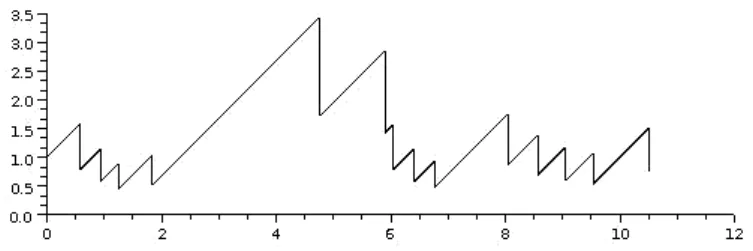
This is a simple storage model: the current stock decreases exponentially and increases by a random amount (divided by the exponential variable) at inhomogeneous random times. The main assumption of this theorem is the contraction of the nucleus in full variation (point iii)).
Examples and applications
Stochastic models for population dynamics
But when r is constant and the curvature ρ is positive, we have g < −rR01log(h)H(dh). With this formula, we can derive the long-term behavior and the contraction properties of the medium measure.
TCP window size process
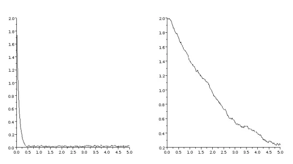
Let (ˆXn)n≥0 be the embedded TCP process chain. 2.16) This Markov chain is often easier to study than the continuous time process. Now, applying [Dav93, Theorem 34.31], we can derive the invariant law of the continuous time process.
Integral of Lévy processes with respect to a Brownian motion
This theorem gives a bound for the coarse Ricci curvature [Oll10], which is the discrete time equivalent of the Wasserstein curvature. This class of Markov processes is reminiscent of the so-called iterated random functions [DF99] or branching processes in random environment [Smi68] in the discrete time setting.
Two criteria without hypoellipticity assumption
In principle, this condition can be slightly relaxed by the addition of a proportionality constant Ci, provided that the rate of change of the process is assumed to be sufficiently slow. We give the previous theorem and its proof for the sake of completeness and for a better understanding of the more complicated case where it is allowed to depend on its first argument.
Two criteria with hypoellipticity assumption
For example, using the results of [BH12,BLMZ12b], Section 3.4.2 gives results analogous to the two previous theorems, in the special case of piecewise deterministic Markov processes where the only small sets for the underlying dynamics consist of a few points to exist. Section 3.4.1 provides sufficient conditions to verify our main assumption in the special case of diffusion processes.
Constant jump rates
Construction of a Lyapunov function
However, Vx0 does not belong to the generator domain in general, as can already be seen in the example of simple Brownian motion. Now we are able to prove that it possesses a Lyapunov function in the case where the switching rates do not depend on the location of the process.
Proof of Theorem 3.1.4
By now imitating the proof of [HM11, Corollary 4.10], we can prove the existence of an invariant measure. More precisely, let us fix a probability measure µ, using the previous inequality we can prove that (µPn)n≥0 is a measure-valued Cauchy series (with respect to the Wddistance).
Proof of Theorem 3.1.7
A set A ⊂ X is small for the semigroup(Pt)t≥0 over a Polish space (X, dX) if there exists a time >0 and a constantε >0 such. Let (Pt)t≥0 be a Markov semigroup over a Polish space (X, dX) such that there exists a Lyapunov function V with the additional property that the sublevel sets {x ∈ X|V(x)≤C} are small for every C > 0.
Non-constant jump rates
- Weak form of Harris’ Theorem
- Construction of a Lyapunov function
- The contracting distance
- Proofs of Theorem 3.1.5 and Theorem 3.3.2
Now we will describe a construction of X that will allow to have a better control of the jumping mechanism. Since I and J can jump only when N jumps, T can only be finite if it is one of the jump times of N.
Two special cases
The case of diffusion processes
Indeed, we can consider that any fundamental Markov process (Zt(i))t≥0 is deterministic, belongs to the space of smooth density functions, and verifies. The previous lemma gives a contraction as in Assumption 3.1.3, for any underlying process, where is the Wasserstein metric.
Case of piecewise deterministic Markov processes
Examples
- The most elementary example
- Wasserstein contraction of some switching dynamical systems
- Surprising blow-up under exponential ergodicity assumptions
- Non-convergence when I is recurrent but not positive recurrent
Cette formule est une généralisation de la formule de Wald dans le cas où les variables ont une dépendance de type branchement. Au chapitre 5, nous commençons par généraliser ces formules dans le contexte qui nous intéresse, puis nous les utilisons pour démontrer des théorèmes de convergence.
Formule de Feynman-Kac et h−transformée
Processus de diffusion de Kolmogorov-Langevin
Un calcul rapide montre maintenant que si ψ satisfait (4.3), alors x 7 → eq(x)ψ(−x) est un vecteur propre du générateur de X.
Processus de Markov modulé
Formule many-to-one
Dans le cas général, G est un opérateur intégro-différentiel et il est difficile de trouver des résultats sur l'existence d'éléments propres. Dans notre cadre, nous avons utilisé les résultats récents de [Per07,DG09, BCnG12] pour l'existence d'éléments propres.
Deux exemples simples de population structurée en taille
Notations
La position de la cellule u est donnée par Xu, sa date de naissance par b(u) et sa date de décès par d(u).
Lorsque r n'est pas constant, cette démonstration ne fonctionne pas, contrairement à la démonstration qui utilise une transformation h. Lorsque r n’est pas constant, le biais n’est pas seulement présent dans le taux de saut.
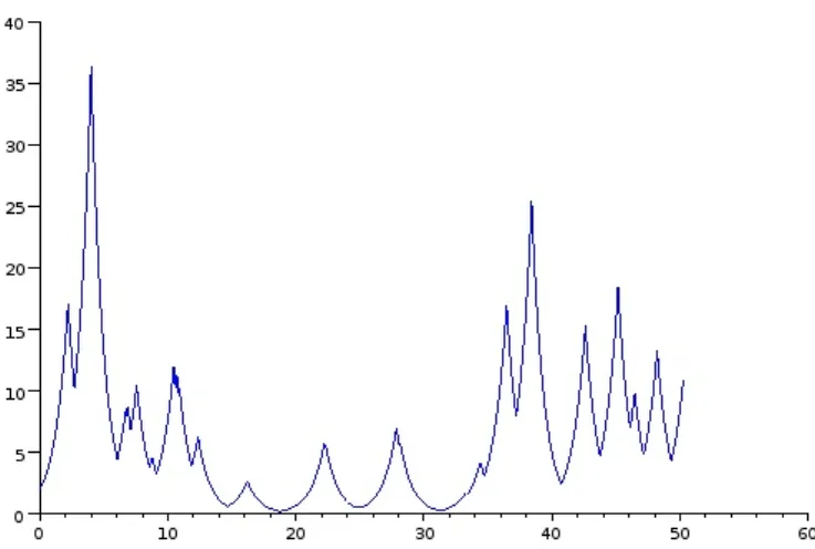
The characteristic of the first individual,(Xt∅)t∈[0,β(∅)) is distributed according to an underlying cadlàg strong Markov process(Xt)t≥0. This model is a branched version of the well-known TCP window sizing process [CMP10,GRZ04,LvL08,OKM96].
Preliminaries
Long time’s behaviour
Eigenelements and auxiliary process
The key point of our weighted many-to-one formula is the anh transformation (Girsanov-type transformation) of the Feynman-Kac semigroup as in [Pin95]. We can see a bias in the drift terms and jump mechanism, which is not observed in [BDMT11, BT11].
Many-to-one formulas
Let (Pt)t≥0 be the semigroup of the auxiliary process; it is defined for every continuous and bounded by. Assuming 5.3.1, if Z0 =δx0, where x0 ∈E, then for all non-negative and measurable functionf, gonE.
Proof of Theorem 5.1.1
Then, due to the first part of the proof, the first term of the sum, on the right, converges to 0 inL2. If h ≡ 1 then all assumptions of the previous theorem apply and we get the first convergence.
Macroscopic approximation
Proof of Theorem 5.1.2
If V is bounded below, we can use the same argument with g = 1 and f = 1/V, which is also a continuous and bounded function. The first point is the tightness of the family of time edges (X(n)t (f))n≥1, and the second point, called the Aldous condition, gives "stochastic continuity".
Main example : a size-structured population model
Equal mitosis : long time behaviour
So we get a many-to-one formula with an auxiliary process generated by Abe defined, for each f ∈Cc2(E)andx∈E, by. But conditioning on the time of the first division and taking the limit t → +∞ yields %2.
Homogeneous case : moment and rate of convergence
By homogeneity, we can see our measure of branchingZas a process indexed by a Galton-Watson tree [BDMT11]. More precisely, since the branching time does not depend on the position, we can set the same times for our two processes.
Asymmetric mitosis : Macroscopic approximation
Since the signed measure set is not metrizable, we cannot adapt the proof of Theorem 5.1.2. Following [M´98,Tra06], we consider η(n) as an operator in a Sobolev space and use the Hilbertian properties of this space to prove tightness.
Another two examples
Space-structured population model
But in this case the auxiliary process is not ergodic and we cannot derive any convergence from our main theorem. If the state space of E is bounded, then we can find sufficient conditions for the eigenproblem in [Pin95, Section 3] and [Pin95,.
Self-similar fragmentation
The article [Clo11] also shows that the empirical process, when the size of the population tends to infinity, converges to the following. The infimum to the right of the last expression is reached in a unique α ≥ 0.
Preliminaries
Behavior of one cell line
Scaling property and application to the study of the size of the largest individual164
Due to the increasing size of the divisions, our situation is different from [Ber06]. There exists a unique α∗ ∈R such that the function α7→λα is convex on R, decreasing on (−∞, α∗) and increasing on (α∗,+∞).
Asymptotic of the largest individual
Exponential increasing for the size of the largest individual
Finally, since mappingp7→α(p) is increasing and mappingα7→βp(α) is decreasing, taking the limit asp→1, we derive the announced result.
Proof of Theorem 6.1.1
Mean behavior of the population
Many-to-one formula and auxiliary process
Proof of Theorem 6.1.2
Denoting Vt(j) the set of cells alive at time issued to the cell, we have.
Fluctuation of the largest individual via deterministic method
In particular, if A is the generator of the Brownian motion and the distribution is dyadic and local, then we find the classical F-KPP equation.