Compared to previous DSD formulations presented in the literature, the presented approach explicitly considers the prefactors of power-law models to produce a uniform and dimensionless scaled distribution, regardless of the reference moments. are proposed to estimate climatological parameters in DSD formulations with one- and two-moment scaling. Water is one of the most valuable natural resources for the development of human society.
The C´evennes-Vivarais region
Description of the C´evennes-Vivarais region
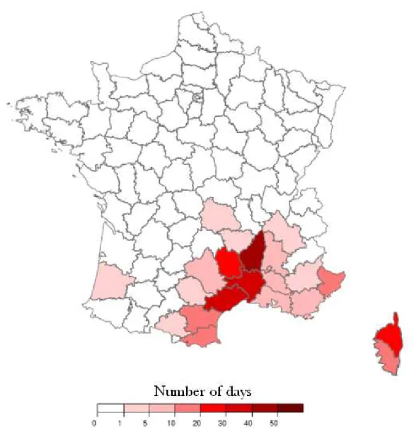
The location of the C´evennes-Vivarais region and its orographic features are extremely favorable for heavy rainfall. All these conditions lead to heavy Mediterranean rainfall (Smith, 1979) that occurs regularly in the C'evennes-Vivarais region, which in French also takes its name from the meteorological and orographic effect of the intense precipitation, called 'episodes'. c´evenols”.
Flooding vulnerability
The transfer of heat and moisture from the Mediterranean Sea colliding with the cold air from the north creates favorable conditions for heavy precipitation (Nuissier et al., 2008). Gard, Loz`ere 828 mm of rain measured during 24 hours at the foot of Mont Aigoual.
Microstructure of rain
- Raindrop size distribution (DSD)
- Parameterization of the DSD
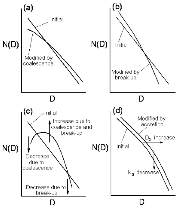
- Evolution of the DSD and microphysics processes
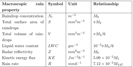
- Relationships among the DSD moments
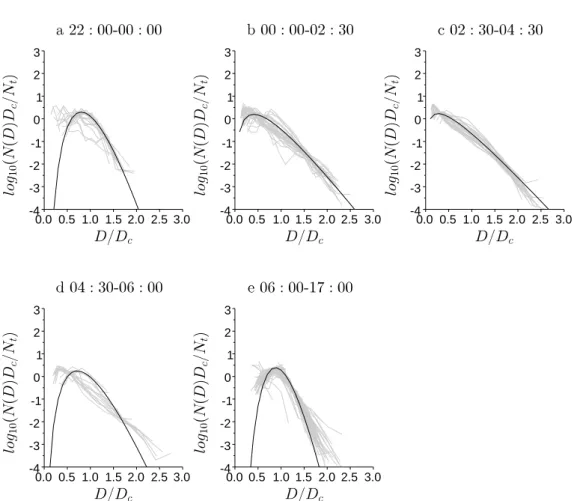
The purpose of scaling analysis is to normalize the variability of DSD by moment(s). The figure illustrates the evolution of the DSD associated with the scaled distribution within 7 rain phases (Chapon et al., 2008).
Meteorological observations of intense precipitation
C´evennes-Vivarais Mediterranean Hydro-meteorological Obser-
The unusual character of the two-moment scaling framework can be seen in the moment relation (1.13), in which the exponents of the two-power relation are determined by the moment orders chosen. Therefore, the DSD formulation plays the role of a bridge connecting the current relationship with the physics of rain.
Description of the meteorological dataset
The observatory focuses on a window of 160 × 200 km2 (Figure 1.6), in which the observing system includes (i) three operational weather radars belonging to the M´et´eo-France ARAMIS network; (ii) 400 daily rain gauges and 160 hourly rain gauges provided by three organizations (M´et´eo-France, Service de Pr´evision des Crues du Grand Delta, Electricit´e de France); (iii) 45 water and discharge stations; (iv) 2 “Parsivel” laser optical disdrometers (Delrieu et al., 2005). The online system (www.ohmcv.fr) for data extraction and visualization was designed and supported by LTHE (Boudevillain et al., 2011).

Recent remote-sensing technologies
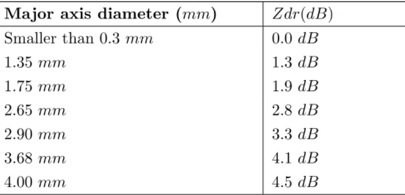
Due to the different shapes of hydrometeors, the attenuation of horizontal and vertical pulses causes a phase shift. Unlike Zdr, this phase shift is not only influenced by the shape of the hydrometeors, but is also related to the concentration of the hydrometeors.
Objectives of this thesis
Number of free parameters in DSD formulations
And thanks to this limitation, the variation in the DSD spectrum is able to be analytically described by several (one to three) parameters. The variation in the DSD spectra is assumed to be determined only by the DSD moments. How many free parameters or moments are required in the DSD parameterization is a core question.
Therefore, the number of free parameters required in the DSD analytical expression is expected to be between 2 and 3.
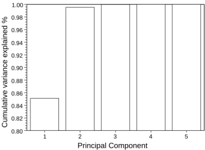
Principal component analysis on the DSD moments
The result of the PCA shows the significant increase in the explained variance if the second (independent) principal component is used. The first three coordinates of the PCA are shown in Fig.2.3, illustrating three basic patterns of the log-transformed DSD moments. Based on PCA theory, all log-transformed DSD moments can be reconstituted by the linear combination of these patterns.
Regarding the reconstitution of the first principal component (Fig.2.4), the intermediate moments, such as M4 and M5, are well reconstituted, while the reconstitutions of the low and high moments, e.g.
Interpretation of the principal components
DSD formulation scaled by concentration and characteristic diameter
- DSD formulation
- Parameter estimation procedures
- Effects of the DSD truncation
- Evaluation of the DSD model scaled by N t and D c
- Climatological characteristics of the DSD
The approximation of the truncated moment (MkT run) to the full moment (Mk) gives a bias in the parameter estimation. The comparison of µ estimated with truncated and full moments is illustrated in Fig. 2.12. Rain intensity clearly depends on the number of medium-sized raindrops (between 1 and 2 mm), while the radar reflectivity factor is mainly contributed by large raindrops (between 2 and 4 mm).
The contributions to the R in (a), and Z in (b), are illustrated as a function of the droplet diameterD.

Interpretation of parameters in the DSD formulation scaled by N t and D c 60
- Links between scaling DSD formulation and the classical gamma
- Formulation
- Parameter estimation procedure
- Evaluation of the two-moment formulation
And the self-consistency relation (2.17) reflects the instinctive constraint between the mean and the standard deviation of the scaled DSD. However, the introduction of the characteristic diameter (Dc) in the DSD formulation turns the cutoff parameter (λg) into a dimensionless parameter (λ), which is related to the shape parameter (µ) by a simple self-consistency relationship. 3.2) Substituting Nt and Dc in the DSD scaling formulation (2.13) from the above power-law relations gives the expression of the two-moment DSD scaling formulation as,.
Due to the uncertainty in the measurement of Nt and the weak relationship between the concentration (Nt) and the predictor moments (R and M6),.
One-moment scaling DSD formulation
Formation
This result highlights the limitation of higher-order moments for estimating lower-order moments. Two climatological DSD models derived by different estimators are evaluated by the correlation coefficient in (a) and the bias in (b). Reconstructed moments based on two climatological DSD models are evaluated separately from the correlation coefficient in (a) and the bias in (b).
Consequently, there are three free parameters to be determined for the single-scaling DSD formulation.

Parameter estimation procedure
Fig.3.9a and 3.10a show the exponents as a function of moment order, for DSD formulations scaled with M3.67 and M6 respectively. The two evaluation methods (based on simple regressions or on all consecutive DSD moments) are performed to obtain the climatological parameters for the DSD formulation scaled by M3.67 and M6, respectively. It appears that the choice of estimation method has a significant impact on the shape parameter (µ).
This bias is significantly reduced in DSD spectra scaled by M6, especially when "simple regression".

Evaluation of one-moment formulations
The black and blue curves represent the DSD models, parameterized by “regression” and “all-moment”. The correlation coefficient and bias between the modeled and observed N(D) are shown in (a) and (b). The black and blue curves represent the DSD models parameterized by "regression" and "all-moment". Thus, the “all moments” estimator is selected for the DSD formulation, scaled based on the rain rate.
The black and blue curves represent the DSD models parameterized with “regression” and “alt-moment” methods, respectively.

DSD scaled by different moment(s)
Comparison of the climatological g(x) scaled by different moment(s) 85
Each figure shows the standard deviation of the scaled distributions by the black bars. It is hoped that the variation of the g(x) function can be reduced as much as possible by the scaling procedure. The M3.67 scaled process reduces the variability of the scale distribution for the medium-scaled diameter range (0.5< x <1.8).
The objective is to show the performance of the scaling DSD formulation in the practical rain event analysis.

Rain event description
The observations in the upper part of the air with the radiosonde at Nˆımes (about 40 km away from Al`es) are presented in Figure 4.4. Duffourg and Ducrocq (2011) emphasized the role of moisture flux from the Mediterranean Sea during the initial and mature phases of a rain event. This moisture flux was lifted up to the top of the troposphere (10 km) in the core of the convective parts.
The y-axis represents the size of the raindrop, and the color refers to the number of raindrops.

Variation of the DSD and rain phases within the event
At this time, the center of the convective system arrived at Al`es and produced most of the rainfall. The most notable variation in the DSD observations was the increase in raindrop concentration up to 2000 m−3, while the Dcand µ remained relatively stable compared to the previous phase. The fifth (last) phase of rain occurred during the day of the 22 and lasted several hours.
As predicted by the evolution of the shape parameter (µ), we find two contrasting shapes between strong convective phases (such as phases 2 and 3) and weak convective phases (such as phases 1 and 5).
Investigation of the rain phases based on remote sensing obser-
The vertical cross-section of the reflectivity factor confirms that the increase in concentration at the end of phase 2 is associated with the arrival of the convection system. Fig.4.15 shows the time series of (1) the height at which the reflectance reaches 30 dBZ and (2) the maximum vertical reflectance values. It appears that the maximum value of the reflectance profile is related to the characteristic diameter measured on the surface, especially when.
The 30dBZ reflects the vertical extension of the deposited system, and the maximum Z is an indicator of the convective activity.

Reconstitution of the DSD by the observed moments
Reconstitution of the DSD
However, the deduction of DSD concentration from radar observations is still a challenge to be overcome in the future. 4.3) These expressions assume that the variation in DSD is fully controlled by rain rate and/or radar reflectivity. Evaluations are performed to compare the reconstructed DSDs with observations based on the entire 5-min DSD data set in Section 3.1.3 and 3.2.3.
However, these estimates were made in the context of a pure DSD study, in which Z and R are also derived from DSD.
Application of the DSD reconstitution on a rain event
The rain intensity and reflectivity factor are derived from the disdrometer (black lines) and derived from radar and rain gauge observations (blue lines). Rain intensity is derived from the disdrometer (black lines) and derived from rain gauge observations (blue lines). Figure 4.20 shows the performance of DSD models reconstructed by the moments derived from the disdrometer.
And the reflectance factor reconstructed DSD model produces a better performance for raindrops larger than 3 mm compared to the rain intensity scaled DSD model.

Estimation of the rainfall erosion energy
- Introduction of the soil erosion by rainfall
- Estimation of the KE based on DSD data
- Application of the KE estimators on a rain event
- Toward the spatialization of rainfall kinetic energy flux density . 125
Four criteria (Bias, N ash, RM SD and R) are used to evaluate DSD models as a function of drop diameter. Recall that the kinetic energy is proportional to the 5th moment of the DSD. The difference in performance reported between Table 4.1 and Table 4.3 must be explained by the error of the DSD model.
Rain gauge icons are colored as a function of KE values derived from observed rainfall.

Extension of the scaling DSD formulation to include the one- and two-
The climatological DSD characteristics of the C´evennes rainfall are revealed by the histograms of three DSD parameters. Finally, a significant improvement of the model performance is obtained if two reference moments are taken into account in the scale formulation. For the DSD formulation jointly scaled by R and Z, the variation of the raindrops between 1 mm and 5 mm is well represented by the model.
Fairly good agreement was observed regardless of the moment(s) used, even in the case of the climatological data set, which, as mentioned above, shows high variability.
Applications of the scaling DSD formulations
Thanks to the definition and the parameter estimators of the general distribution, our approach offers the possibility to compare the g(x) functions obtained by different moment(s). It is clear that the spectra with large drops are better scaled by the high-order moment and the variation in small raindrops is reduced if low-order moments are taken into account in the scaling process. convective system has a different behavior compared to that in the center of the convective area. Consequently, the movement of the convective system towards the disdrometer resulted in different DSD phases recorded in time series.
The efficiency of the estimation can be improved if the rain gauge data is used together with the radar reflectivity in the estimation.
Prospective
Improving the DSD formulation
Based on the results shown in Fig.2.18, the gamma function may no longer be able to represent the function thef(x) if >0.
Hydrometeorological applications
Mualem, 1989: Regional rainfall similarity: a dimensionless model of the drop size distribution. Transactions of the ASAE. Boudevillain, 2008: Variability of raindrop size distribution and its effect on the Z - R relationship: A case study for intense Mediterranean rainfall. Nakamura, 2001: Characteristics of raindrop size distributions in tropical continental squall lines observed in Darwin, Australia.
W., 1985: Effects of truncation of drop size distributions on integral parameters and empirical precipitation relations.
Topographic map of the C´evennes-Vivarais region in Southern France
Number of heavy rain days during the recent 30 years (1979-2008) for
Intra-variability of the DSD within one rain event
Schematic diagrams illustrating the effects on the raindrop size distribu-
Schematic diagrams illustrating the effects on the raindrop size distribu-
Location of the CVMHO C´evennes–Vivarais window in France
Cumulative precipitation measured by raingauge and disdrometer during
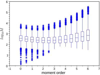
Boxplot of the log-transformed DSD moments for the 5-min data
Cumulative variability explained by the principal components
First three patterns of the DSD in the PCA
Reconstitution of log-transformed DSD moments based on the first prin-
Reconstitution of log-transformed DSD moments based on the first two
Reconstitution of log-transformed DSD moments based on the first three
Relationship between the two parameters (µ and λ)
Comparison of µ derived from different estimators for the climatological