Observateurs d'intervalle pour les systèmes en temps continu, non linéaires et affines dans les variables non mesurées [36]. Observateurs à intervalles continus-discrets pour systèmes à temps continu avec sortie constante par morceaux [92,93].
Introduction
On rappelle les observateurs classiques tels que l'observateur de Luenberger, le filtre de Kalman, le filtre de Kalman étendu, les approches "high gain", et les observateurs continus-discrets. Enfin, nous présentons un type particulier d'observateurs appelés observateurs à intervalles pour les systèmes à temps continu et à temps discret.
Contrˆ olabilit´ e et observabilit´ e de syst` emes lin´ eaires
- Observabilit´ e de syst` emes discrets
- Observabilit´ e de syst` emes continus
- Contrˆ olabilit´ e de syst` emes discrets
- Contrˆ olabilit´ e de syst` emes continus
Le système linéaire en temps continu (1.7) avec la mesure (1.8) est observable si et seulement si la matrice d'observabilité a un rang complet. Le système linéaire en temps continu est contrôlable si et seulement si la matrice de contrôlabilité C a un rang complet, c'est-à-dire rangC=n.
Stabilisation, feedback
Notions de stabilit´ e
Le système (1.33) est dit un état d’entrée stable (ISS) s’il existe une fonction β de classe KL et une fonction γ de classe K∞ (appelée gain ISS), telles que pour toute condition initiale x0 ∈Rn et une entrée arbitrairement admissible u , sa solution satisfait Le système (1.33) est dit complètement stable par rapport à l’état d’entrée s’il existe une fonction β de classe KL et deux fonctions µ1, µ2 de classe K∞, telles que pour chaque condition initiale x0 ∈Rn et toute entrée admissible vous sa solution satisfait.
Le retour d’´ etat
Une alternative à l'ISS est la stabilité intégrale d'entrée à état (iISS), introduite dans [128], qui estime l'énergie d'effet du signal appliqué (au lieu de son amplitude) sur le système considéré. Lorsqu'on veut stabiliser exponentiellement le système (1.34), on peut déterminer le gain K tel que A+BK soit Hurwitz.
M´ ethode de Lyapunov et technique d’ajout d’int´ egrateur
Nous montrons ensuite que le système est asymptotiquement stable si et seulement s'il existe une matrice P = P>0 telle que la LMI suivante (également appelée inégalité de Lyapunov) contient ee. Cette approche aborde essentiellement le problème de la construction d’une rétroaction qui stabilise globalement asymptotiquement l’origine d’un système façonné donné.
M´ ethodes d’estimation d’´ etat classique
- Observateur de Luenberger
- Filtre de Kalman
- Approches ”grand gain”
- Observateur continu-discret
En revanche, ils ne sont applicables qu’à une classe limitée de systèmes non linéaires. Dans [31] les auteurs établissent les résultats de stabilité pour les filtres de Kalman étendus dans le cas de systèmes continus à mesures continues (systèmes continus-continus), ainsi que dans le cas de systèmes continus à mesures discrètes (systèmes continus-discrets) de l'observateur intégré dans [48].
Syst` emes monotones et positifs
Les syst` emes positifs
A= (aij) ∈Rn×m est une matrice positive si ∀i, j :aij ≥0, autrement dit toutes ses entrées sont positives. Le système (1.77) est positif si et seulement si A est une matrice de Metzler et b≥0.
Principe des syst` emes coop´ eratifs
Th´ eor` eme de Birkhoff
Observateurs par intervalles bas´ es sur la th´ eorie des syst` emes coop´ eratifs
Version ` a temps continu
Si si est coopératif, alors le système différentiel suivant encadre les solutions du système (1.90). Si la matrice A ∈ Rn×n est coopérative, alors le système différentiel suivant est entre les solutions du système (1.93).
Version ` a temps discret
Si la matrice A∈Rn×n est une matrice de stabilité au sens de Schur, c'est un observateur d'intervalle. De plus, dans le cas où wk= 0, le système ez+k+1−zk+1− =A(zk+−zk−) est globalement asymptotiquement stable car la matrice A ∈Rn×n est une matrice de stabilité au sens est originaire de Schur.
Conclusion
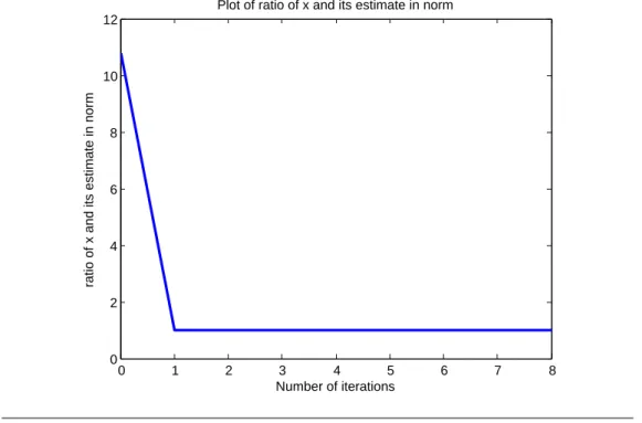
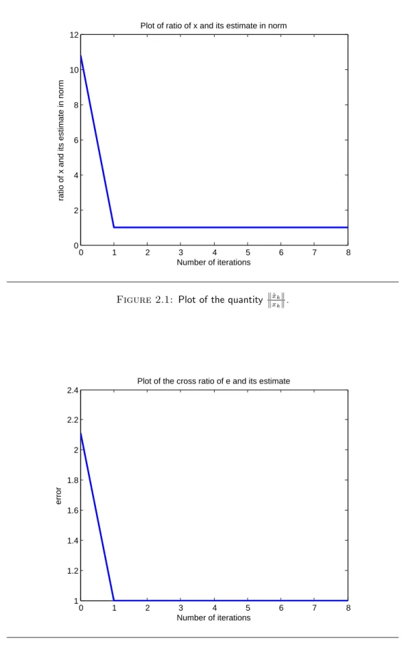
Once the direction of the true state is correctly estimated (i.e., the state is correctly estimated in the projective space), very mild assumptions on the output map allow its norm to be reconstructed and thus the entire state to be estimated. Once the direction of the error is correctly estimated, its norm can be estimated again.
Positive linear systems and the Birkhoff theorem
This means that for two arbitrary solutions xk,x˜k we have d(xk,x˜k)≤γkd(x0,x˜0). Note that the celebrated Perron-Froebenius theorem can be seen as a consequence of the Birkhoff theorem as in the projective spaceAis turns out to be a contraction. As a final remark, note that the contraction rate is monotonically linked to the diameter of the card A: a smaller diameter ensures a higher contraction rate.
A class of positive observers for positive systems
Nonlinear Luenberger type positive observers for positive linear systems 47
Then, due to the assumption that w0< x0, and from assumption (a), we have it always positive. First, the theorem indicates the convergence of the estimation error to zero in generalized polar coordinates.
Gain tuning issues
Optimization problem involved
It is a minmax optimization problem and can be numerically handled through standard optimization methods, including brute force algorithms if the state space dimension is not too large.
A geometrical method to decrease ∆(A + LC)
Two-dimensional linear case
Illustrative example
Conclusion
The aim of the present chapter is to complement the design techniques of interval observers available for this type of system, and in particular [116]. This fact may sound surprising since most of the designs of interval observers available in the literature are performed for cooperative systems (sometimes after a coordinate transformation).
Notation, definitions, basic result
It is interesting in itself because it gives conditions that ensure that the system is non-negative without implying that it is cooperative.
A new interval observer design
One can easily check if an inputu is such that all solutions of the system (3.1) are defined over [0,+∞) and belong to a compact set, then lim. We establish the global asymptotic stability of the origin of the system (3.17) through a Lyapunov approximation.
Illustrative example
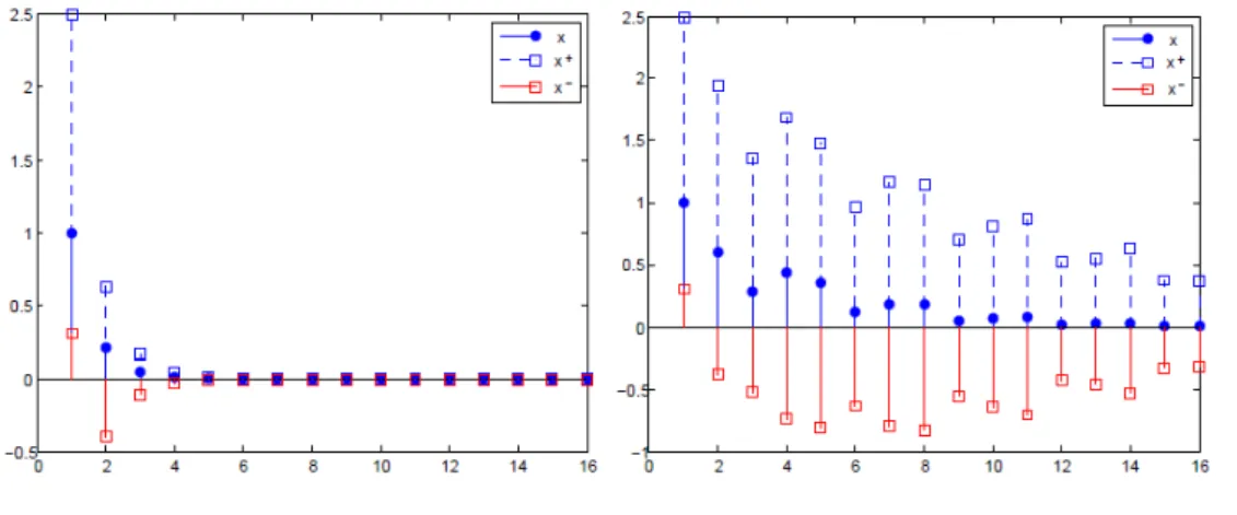
Figure 3.2 below shows that in the case where the system is affected by additive disturbances, the interval observer still provided the solutions with bounds, which do not converge to the solution of the studied system. The initial conditions we chose are the same as those chosen in the undisturbed case of Figure 3.1.
Conclusion
In Section 4.3 we state and prove results of constructing interval observers for nonlinear systems. A construction of time-varying interval observers for linear systems with outputs is proposed in section 4.5.
Notation, definitions, basic result
Finally, let us note that the paper [38] differs from our work presented in this chapter for the following reasons: (i) The first main result of [38] is devoted to time-invariant linear systems with outputs and relies on a observability condition that guarantees the existence of time-invariant coordinate changes leading to equations for which interval observers can be easily constructed. ii) The second main result of [38] is devoted to time-varying linear systems. In Section 4.4, we state and prove that any discrete-time, exponentially stable, time-invariant linear system can be transformed into a block diagonal system with nonnegative and exponentially stable subsystems.
Time–invariant interval observers
Interval observers for nonlinear systems
Extending Theorem 4.4 to the case where the time-varying system (4.9) can be obtained. To begin with, we note that the existence of functions θc, ρc that satisfy the conditions of Theorem 4.6 is a consequence of Lemma A.4 in A.
Interval observers for linear systems
Transformations of linear systems into nonnegative systems
Next, we will focus our attention on the fundamental family of linear time-invariant discrete-time systems. The construction we will propose relies on time-varying changes of coordinates that transform linear discrete-time systems into nonnegative discrete-time systems.
Time-varying interval observers
The proof idea: first, we recall that every real matrix admits a real Jordan canonical form.
Illustrative examples
Nonlinear system
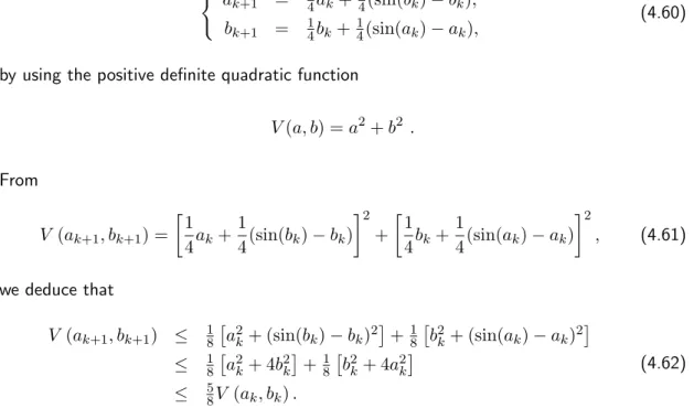
Since V is a positive definite quadratic function, we conclude that system (4.60) accepts the origin as a globally exponentially stable equilibrium point. The simulations confirm the mathematical result: in the absence of perturbation, there is convergence of the two solution bounds, and in the presence of perturbation, the bounds do not necessarily converge to the same value.
Linear system
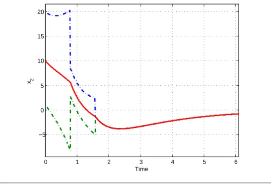
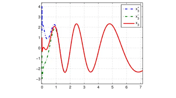
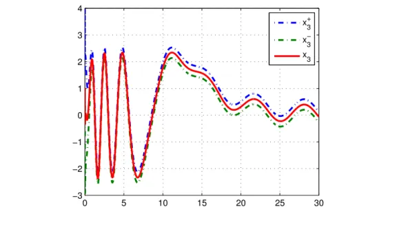
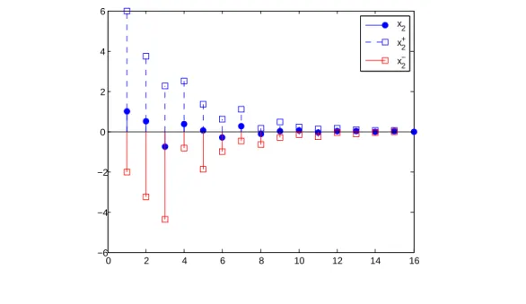
Figure 4.3 shows the second component of x and the limits provided by an interval observer in the absence of interference. The simulations confirm the theoretical result: in the absence of disturbances, the convergence of both limits of the solution occurs, but in the presence of disturbances, the limits do not necessarily converge to the same value.
Conclusion
We give some sufficient conditions ensuring that the system can be exponentially stabilized by a dynamic output response depending on yk and the values provided by the interval observer limits. Thus, better estimates can be obtained without having to consider range observers of dimension greater than twice the dimension of the studied system.
Notation, definitions and prerequisites
Interval observer
Note for later use that Assumption 5.1 guarantees the existence of a symmetric positive definite matrix Q∈Rn×n such that. With assumption 5.2 in mind, we easily derive that when the disturbances are present, there is a constantn>0 such that. 5.49).
Illustrative example
With assumption 5.2 in mind, we easily derive that when the disturbances are present, there is a constantn>0 such that. 5.49) The triangle inequality suggests that. Next, figure 5.2 shows the solution with the same initial conditions in the case where the system is affected by disturbances ςj = 8.
Conclusion
Extensions of the results to families of time-varying systems with discrete time and delays and their fitting to the continuous-time case can also be expected. It is worth pointing out that the estimators we propose are not directly derived from the interval observers constructed for continuous-time systems in [89] and for discrete-time systems in [38] or Chapters4, although some of the main ideas of these works are used along our construction.
Notation, definitions
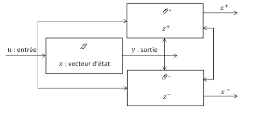
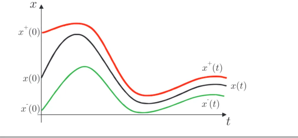
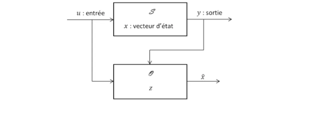
After constructing interval observers for both continuous-time and discrete-time systems, a question about interval observer design for continuous-time systems with discrete measurements naturally arose and the last chapter of the thesis was devoted to the solution of this problem. These interval observers are composed of two copies of the studied system and of a framer. In the last ten years or so, the design of positive observers for positive systems (i.e. observers such that the estimated state respects positivity) has attracted an ever-growing attention.
Moreover, the design of interval observers for continuous-time systems with discrete measurements is another nice problem to solve.