MŰHELYTANULMÁNYOK DISCUSSION PAPERS MT-DP – 2009/13
Monetary Transmission in Three Central European Economies:
Evidence from Time-Varying
Coefficient Vector Autoregressions
ZSOLT DARVAS
Discussion papers MT-DP – 2009/13
Institute of Economics, Hungarian Academy of Sciences
KTI/IE Discussion Papers are circulated to promote discussion and provoque comments.
Any references to discussion papers should clearly state that the paper is preliminary.
Materials published in this series may subject to further publication.
Monetary Transmission in Three Central European Economies:
Evidence from Time-Varying Coefficient Vector Autoregressions
Zsolt Darvas senior research fellow Institute of Economics Hungarian Academy of Sciences,
Bruegel, Brussels
Corvinus University of Budapest E-mail: darvas@econ.core.hu
July 2009
ISBN 978 963 9796 64 5 ISSN 1785 377X
Monetary Transmission in Three Central European Economies: Evidence from Time-Varying
Coefficient Vector Autoregressions
Zsolt Darvas
Abstract
This paper studies the transmission of monetary policy to macroeconomic variables in three new EU Member States in comparison with that in the euro area with structural time-varying coefficient vector autoregressions. In line with the Lucas Critique reduced-form models like standard VARs are not invariant to changes in policy regimes. The countries we study have experienced changes in monetary policy regimes and went through substantial structural changes, which call for the use of a time-varying parameter analysis. Our results indicate that in the euro area the impact on output of a monetary shock have decreased in time while in the new member states of the EU both decreases and increases can be observed. At the last observation of our sample, the second quarter of 2008, monetary policy was the most powerful in Poland and comparable in strength to that in the euro area, the least powerful responses were observed in Hungary while the Czech Republic lied in between.
We explain these results by the credibility of monetary policy, openness and the share of foreign currency loans.
Keywords:
monetary transmission, time-varying coefficient vector autoregressions, Kalman-filter
JEL: C32, E50
Acknowledgements:
I am thankful to Fabio Canova, Peter van Els, Leo de Haan, Benoît Mojon, András Simon, Peter Vlaar, an anonymous referee at De Nederlandsche Bank, seminar participants at De Nederlandsche Bank, Magyar Nemzeti Bank and Oesterreichische Nationalbank, and conference participants at the ECOMOD and at the Annual Congress of the European Economic Association for comments and suggestions. Part of this research was conducted while I was a visiting scholar at De Nederlandsche Bank, whose hospitality is gratefully acknowledged.
The views expressed in this paper do not necessarily represent those of De
Nederlandsche Bank. Financial support from OTKA grant No. K76868 is also
acknowledged.
Monetáris transzmisszió három közép-európai országban: becslés időben változó paraméterű
vektor autoregresszió segítségével
Darvas Zsolt
Összefoglaló
A tanulmány a monetáris politika transzmissziós mechanizmusát vizsgálja a fő makrogazdasági változókra Csehországban, Magyarországon és Lengyelországban az euróövezettel összevetésben, időben változó paraméterű vektor autoregresszió (VAR) segítségével. A Lucas-kritika alapján a redukált formájú modellek, mint például a szokásos VAR-modellek, nem invariánsak a gazdaságpolitikai változásokra. A vizsgált országokban a monetáris politika keretrendszere változott a rendelkezésre álló mintaperiódusban, valamint számottevő strukturális változások is történtek, amelyek szükségessé teszik az időben változó paraméterű modellezést. Eredményeink azt jelzik, hogy az euróövezetben a monetáris politika reálgazdasági hatása mérséklődött az elmúlt években, míg a három vizsgált új EU-tagországban mérséklődés és erősödés is megfigyelhető. A mintaperiódusunk utolsó időpontjánál, 2008 második negyedévénél a monetáris politika hatása Lengyelországban olyan erős volt, mint az euró övezetben, Magyarországon jóval gyengébb volt, Csehországban pedig a hatás erőssége ezen két ország értékei között helyezkedett el. Eredményeinket a monetáris politika hitelességével, a gazdaság nyitottságával és a devizahitelek arányával magyarázzuk.
Tárgyszavak: monetáris transzmisszió, időben változó paraméterű vektor
autoregresszió, Kálmán-szűrő
JEL: C32, E50
1. INTRODUCTION
The monetary transmission mechanism shows the effects of monetary policy on key macroeconomic and financial variables. Analysis of the monetary transmission mechanism has a central role in macroeconomic policy research and is crucial for the conduct of monetary policy. A good understanding of the transmission mechanism is especially important for the implementation of inflation targeting, because without that the inflation can not be targeted well and as the transmission mechanism changes, the reaction function of monetary policy should also change even if the preferences of the central bank are unchanged.
The transmission mechanism of monetary policy also has implications for euro adoption and proper functioning within a monetary union. The relevance of the monetary transmission mechanism from the perspective of euro adoption is that when the effects of domestic monetary policy on inflation and output are large and very different from the effects observed in the euro area, then the cost of loosing monetary policy independence might be significant. In the opposite case, the loss is less important. On the other hand, similarity of the transmission mechanism across member states of a currency area is important. Ideally, monetary policy should have the same effect on all member states, causing them to share the burden of adjustment after a monetary contraction or the advantages of a monetary easing equally. Analysis of the transmission mechanism for countries currently outside the monetary union can give insights into euro adoption considerations but has less relevance for the question on proper functioning inside a monetary union, because the transmission mechanism may change after the entry into the monetary union.
The Monetary Transmission Network of the European System of Central Banks (ESCB) analyzed in detail the transmission mechanism in the current euro area member countries (Angeloni et al., 2003). A large amount of research has also been conducted for the New Member States (NMS) of the EU; see Égert and MacDonald (2008) for an extensive survey.
However, studying the NMS with standard techniques raises an elementary problem that is related to time varying parameters. First, both common sense and the Lucas Critique suggest that changes in monetary regimes are likely to affect the transmission of monetary policy.1 For example, a shift from exchange rate targeting to inflation targeting may weaken exchange rate pass-through, because an exchange rate change can be regarded as permanent in the
1 Furthermore, most previous studies adopted reduced-form and linear models for the analysis. For example, the vector autoregression (VAR) methodology is perhaps the most common econometric tool for the study of the transmission mechanism (see Christiano, Eichenbaum and Evans, 1999) that is typically used to study the transmission to key macroeconomic variables. The parameters of reduced-form models are not invariant to policy changes.
former but not in the later regime. During the last decade a number of NMS, like the Czech Republic, Hungary and Poland, made their exchange rate regimes more flexible and changed the way of conducting monetary policy, reaching an inflation targeting framework at the end.
Regime changes call into question the usefulness of studying the available sample period of these countries with fixed parameter models. Only a few years have passed since the last change in regime and the period since the last change does not provide a sufficient number of observations for estimation.2
Second, these countries have undergone substantial structural changes since their transition from the socialist economic system in the early nineties and these changes might have effected the parameters of response function of monetary policy even if the regime was unchanged.
Third, the parameters of linear models (which are typically used) can change even if the underlying structural model has constant parameters, provided that the underlying structural model is nonlinear. In a recent paper Granger (2008) also advocated the use of time-varying parameter techniques.
Despite the above-mentioned drawbacks, to our knowledge this paper is the first to adopt time-varying coefficient (TVC) techniques for studying the transmission mechanism of some NMS.3 Still, possible time variation in the transmission mechanism or time variation in the variance of shocks hitting the economy is certainly not only an NMS issue. There is a heavy debate about the monetary policy of the U.S.A.; see, for instance, Canova and Gambetti (2006), Cogley and Sargent (2005), Sims and Zha (2006) and references therein. Canova and Gambetti (2006) question whether U.S. inflation is the result of “bad luck or bad policy,” that is, whether the bad inflation outcome of the early 1980s and the good inflation outcome since the late 1980s are due to “luck” (the decline in the variance of the shocks) or to “policy”
(changes in the way monetary policy is conducted). They found more evidence in favour of the bad luck hypothesis, while Cogley and Sargent (2005) support the bad policy view.
The empirical results of Primiceri (2005) are also more supportive for the bad luck view since he found that the role played by exogenous non-policy shocks seemed more important than interest rate policy in explaining the high inflation and unemployment episodes in recent U.S. economic history. Regarding monetary policy, he found that responses of the interest
2 Moreover, even since the last major regime change some less pronounced although important changes may have taken place, for example the exchange rate band devaluation of the Hungarian forint in 2003. These minor or sub-regime changes further complicate the selection of sample periods of stable monetary policy regimes and hence constant parameters.
3 The survey presented in Égert and MacDonald (2008) identifies this paper as the only one adopting time-varying coefficient methods for the study of the monetary transmission mechanism in the NMS, in addition to a related paper of Darvas (2001), which studied the exchange rate pass-through using a TVC error-correction model.
rate to inflation and unemployment exhibited a trend toward a more aggressive behaviour, but this has had a negligible effect on the rest of the economy.
For some old EU countries, Ciccarelli and Rebucci (2006) used a TVC technique to study changes in the monetary transmission mechanism in the period of 1981-1998. They found that the long-run impact on output of a common monetary policy shock has decreased after 1991 in all countries studied. Using a more recent sample period, 1980-2007, Boivin, Giannoni and Mojon (2008) found that the creation of the euro has contributed to an overall reduction in the effects of monetary shocks, but also to a greater homogeneity of the transmission mechanism across countries. Using a structural open-economy model they argue that these findings can be attributed to the combination of a change in the policy reaction function (mainly towards more aggressive response to inflation and output) and the elimination of an exchange rate risk.
In this paper we study the transmission mechanism on macroeconomic variables in three NMS, namely the Czech Republic, Hungary and Poland. We also study the transmission mechanism of the euro area to compare the transmission mechanism in the three NMS with that of the euro area as a whole. The method we use is time-varying coefficient vector autoregression (TVC-VAR). Our results indicate that monetary transmission changed in the three countries, as it did in the euro area. In particular, the response of output to a monetary policy shock has declined in the euro area, which finding is in line with Ciccarelli and Rebucci (2006) and Boivin, Giannoni and Mojon (2008). Monetary policy became more effective in time in Hungary and Poland, while the time profile of the change is not monotonous in the Czech Republic. At the last observation of our sample, the second quarter of 2008, we find that among these three countries monetary policy is the most powerful in Poland and comparable in strength (though with a different time profile) to that of the euro area and is the least powerful in Hungary, while the Czech Republic is in between. We explain these differences with the accumulated credibility of monetary policy in the three countries, openness and the share of foreign currency loans.
The rest of the paper is organized as follows. Section 2 briefly describes monetary regimes in the three NMS. Section 3 surveys the TVC-VARs used in the literature and describes the model we use. Section 4 details the data. The results of our TVC-VAR analysis are presented in section 5. Section 6 discusses the results and finally Section 7 presents a brief summary.
2. MONETARY REGIMES IN THE NMS
Figures 1, 2 and 3 show nominal exchange rate developments in the Czech Republic, Hungary and Poland, respectively. The Czech Republic had a narrow exchange rate band regime before 1996,4 when the band was widened to 7.5%. Not much later, in May 1997, the band was swept away by a speculative attack, and the koruna was floated with occasional central bank interventions and inflation targeting was introduced in January 1998.
In Hungary, a pre-announced crawling band regime was introduced in March 1995 after a long period with an adjustable peg. The adopted band was narrow at 2.25%. However, as Figure 2 shows, the market rate eventually evolved like in a crawling peg, since it was almost continuously at the strong edge of the band (with the exception of the period of the Russian and Brazilian crises in late 1998 and early 1999). The band was widened substantially in May 2001 to 15% and inflation targeting was introduced. However, at this time the exchange rate band and its crawling devaluation were kept. The rate of crawl was reduced to zero in October 2001. Following a strong appreciation pressure in early 2003, in June 2003 the band was unexpectedly devalued by 2%. In February 2008 the band was abandoned and free floating was introduced.
The Polish authorities made their exchange rate regime flexible gradually. As Figure 3 indicates, Poland also adopted a pre-announced crawling band for most of the 1990s, but the band was widened to 15% in several steps. There were heavy central bank interventions until 1997, which is also reflected in the relatively stable rate within the band, but since early 1998, the rate was allowed to move freely within the wide band. In April 2000, the band was abolished and inflation targeting was introduced with a freely floating exchange rate.5
Hence, all three countries moved from an exchange rate targeting regime to an inflation targeting system. These changes in monetary regimes definitely had an impact on the monetary transmission mechanism. Estimation for a sample consisting of both the exchange rate targeting and the inflation targeting regimes does not make sense with a fixed parameter model. The longest homogeneous sample is available for the Czech Republic starting in 1998.6 In the cases of Poland and Hungary, the latest major regime change occurred in 2000
4 Figure 1 shows data starting in 1995; up to 1995 the width of the band was similarly narrow.
5 For more information on the exchange rate systems of these countries, see Darvas and Szapáry (2008).
6 This has prompted Borys and Horváth (2008) to use fixed parameter models for the sample period of 1998-2006. However, structural changes not related to changes in monetary policy regimes may have taken place during this period as well. Given
and 2001, respectively, but the band shift of the Hungarian forint in 2003 marked a minor or sub-regime change and the move to a free float in 2008 also marks a change.7 Therefore, the sample periods since the last regime changes are too short for reliable fixed parameter analyses, even if it is assumed that the linear approximation was correct and no structural change have taken place.
3. TIME-VARYING COEFFICIENT VARS
This section discusses five issues related to our methodology: the type of the TVC-VAR, lag length, shock identification, impulse response analysis and initial conditions.
3.1 SPECIFICATION
Three main types of TVC-VAR models have been proposed recent years:
1) Parameters, treated as latent variables, assumed to follow random walks without drift and the Kalman filter is used for estimation.8 This technique was used e.g. in Cogley and Sargent (2005), Primiceri (2005), Canova and Gambetti (2006), and Ciccarelli and Rebucci (2006)9.
2) Parameters switch between regimes (back and forth) driven by a latent state variable which follows a Markov switching process. This technique was used in e.g. Sims and Zha (2006).
the still somewhat limited length of their sample, they decided to work at monthly frequency and interpolate GDP and output gap figures that are available at the quarterly frequency. As they acknowledge, interpolation has some disadvantages.
7 The tiny 2% devaluation compared to the ±15% width of the band in 2003 indicated that monetary authorities had changed their preferences. Up to 2003, the exchange rate had been allowed to reach the strong edge of the band fuelled by high interest rates and revaluation expectations. The devaluation signalled that the authorities did not want to allow a strong nominal exchange rate anymore. In contrast, the abandonment of the exchange rate band in 2008 could have indicated that inflation will receive more attention in the future.
8 See Hamilton, Chapter 13 for an excellent exposition of Kalman-filtering and the maximum likelihood estimation of the parameters of a state-space system.
9 To be more precise, Ciccarelli and Rebucci (2006) did not use a VAR but adopted a two-stage approach. In the first stage they measured monetary policy by estimating a system of reaction functions, and in the second stage they estimated output equations using the first stage estimates of monetary policy. Consequently, they do not model exchange rates and inflation rates.
3) Parameters change from one regime to another smoothly (and permanently) in time; the specification is the multivariate extension of the STAR (smooth transition threshold autoregression) model. This technique was developed in He, Teräsvirta and González (forthcoming).
In this paper we follow the papers indicated in the first group by assuming that reduced- form VAR parameters follow driftless random walks and use the Kalman filter for estimation and inference. The main reason for our choice is that the random walk specification is a flexible model which can capture various time paths of the parameters resulting from policy changes and structural changes in the economy. In contrast, the STAR-type time specification assumes a particular path and a smooth transition between the beginning and the end regime, which could be too restrictive. The Markov switching specification, on the other hand, assumes a certain number of regimes having different (but fixed in time) parameters and that the process switches back and forth between these regimes. Specifying a limited number of states seems less attractive compared to the flexibility of the random walk specification. Nonetheless, it would be interesting to apply the other two techniques as well in a future work for the study of the transmission mechanism of the new member states.
A difference of our work to some of the papers highlighted in the first group is that we use maximum likelihood estimation, while these papers adopted Bayesian techniques.
3.2 LAG LENGTH
A key issue in TVC-VAR analysis is the selection of the lag length. Larger lags require the estimation of a large number of parameters, which is more difficult in a TVC than in a fixed parameter setting. When the order of the VAR is just one, for a four variable VAR sixteen TVCs need to be estimated when the VAR does not include an intercept. This implies sixteen parameters; they are the standard errors of the innovations driving the parameters in the state equations. There are four additional parameters in the measurement equations as well;
they are the standard errors of the innovations of the measurement equations. Hence, in a VAR(1) without an intercept 20 parameters need to be estimated. We found that a VAR(1) is not satisfactory: innovations in some (not all) equations were autocorrelated. Increasing the order of VAR without any constraint would highly explode the number of parameters to be estimated. Consequently, we adopt a certain type of restriction. Stock and Watson (2005), who estimate fixed parameter factor-structural vector autoregression (FSVAR) for the G-7, allow more lags only for the left-hand side variable and restrict the number of lags of all other variables to one. We follow their approach to our TVC-VAR:
t t t t
p t
p t
p t
p t
p t p
t p
t p
t
t t t t
t t t t
t t t t
t t t t
t t t t
t t t t
t t t t
t t t t
v v v v
y y y y
y y y y
y y y y
y y y y
, 4
, 3
, 2
, 1
, 4
, 3
, 2
, 1
) (
, 44 ) (
, 33 ) (
, 22 ) (
, 11
2 , 4
2 , 3
2 , 2
2 , 1
) 2 (
, 44 ) 2 (
, 33 ) 2 (
, 22 ) 2 (
, 11
1 , 4
1 , 3
1 , 2
1 , 1
) 1 (
, 44 ) 1 (
, 43 ) 1 (
, 42 ) 1 (
, 41
) 1 (
, 34 ) 1 (
, 33 ) 1 (
, 32 ) 1 (
, 31
) 1 (
, 24 ) 1 (
, 23 ) 1 (
, 22 ) 1 (
, 21
) 1 (
, 14 ) 1 (
, 13 ) 1 (
, 12 ) 1 (
, 11
, 4
, 3
, 2
, 1
0 0 0
0 0
0
0 0 0
0 0 0
0 0 0
0 0
0
0 0 0
0 0 0
,
where yi,tdenote the variables included in the VAR,
(jkm,)tdenote the time-varying parameters to be estimated, and vi,tdenote the innovations.With the random walk specification for (jkm,)t, the TVC VAR above can be easily written in a state-space representation and the Kalman-filter can be used to evaluate the likelihood function. Following the maximum likelihood estimation the Kalman-filter can also be used to infer the time-varying parameters.
3.3 IDENTIFICATION
A next issue is identification. Traditional identification, which usually takes the form of some contemporaneous and/or long-run restrictions, has been severely criticized.
Contemporaneous restrictions have been criticized on the basis of being ad hoc, while long run restrictions have been shown to entail large estimation error (e.g. in Faust and Leeper, 1997). A possible new way of identifying shocks is the recent sign restriction identification method (e.g. Uhlig (2005), Canova and De Nicoló (2002), and Peersman (2005)). Darvas (2008) found that sign restrictions are more robust than long-run restrictions. Fry and Pagan (2007) on the other hand highlight some drawbacks of the sign restriction methodology and argue for the superiority of contemporaneous restrictions. Due to the inconclusiveness of the debate over various identification techniques, in this paper we use standard contemporaneous restrictions to identify structural shocks. We assume that monetary disturbances do not affect output and prices contemporaneously (we use quarterly data), but instantly affect the interest rate and the real exchange rate.
3.4 IMPULSE RESPONSE ANALYSIS
The fourth issue is impulse response analysis. Since the model is nonlinear due to changing parameters, no unique impulse response function is available, but we can attach an impulse response function to each observation of the sample. Still, there are two possible ways to proceed. One could use the parameter set of time t to calculate the impulse response function for t, t+1, t+2, …, or use the parameter set of time t, t+1, t+2, …, that is, take into account future parameter changes.
The first option answers the question “Given sample data up to time t, what would the estimated transmission mechanism at time t have looked like?”10. The second one answers the question “Given sample data up to now, what would the transmission mechanism of a shock that hit at time t have been?” Obviously, at the last observation of the sample only the first option can be used, at the last but one observation the second option can be used only for one observation, and so on. We used the first option in the whole sample period. In practice, we calculated the impulse responses as the difference between two simulations, a baseline one and one with a shock at time t.
Impulse response functions are usually graphed to show the effects of a one standard deviation shock. Since the volatility of monetary shocks vary across countries and we also aim to compare the results across countries, we normalize the impulse response functions to show the effects of a 100 basis point monetary policy shock.
3.5 INITIAL CONDITIONS
Since the time-varying parameters assumed to follow random walks, they do not have means that could be used as initial conditions. For this reason we estimated a fixed parameter VAR, equation by equation, with OLS for the first sixteen (effective) observations and used these estimates to form initial conditions for the time varying parameters and their covariance matrix. For example, the first equation (when the lag length is 1 and an intercept is not included) is:
t t t
t t
t y y y y v
y1, 11(1) 1,112(1) 2,113(1) 3,114(1) 4,1 1, ,
and let ˆ1 denote the estimated coefficient vector, that is,
14(1)
) 1 ( 13 ) 1 ( 12 ) 1 ( 11
1 ˆ ˆ ˆ ˆ
ˆ
. Let ˆ1 denote the OLS covariance matrix of this estimation. Let us denote the parameter estimates10 Since parameters are assumed to follow driftless random walks, their forecasts are equal to their current values. We use revised and not real time data and for this reason the question above is not equivalent to the question "What did monetary authorities think that the transmission would be?"
and their covariance matrices similarly (with different subscripts) for the other three equations.
a0, the initial condition for the time-varying parameters is set to:
1 2 3 4
0 ˆ ˆ ˆ ˆ
a .
P0, the initial condition for the covariance matrix of a0 is set equal to the block diagonal matrix formed from the OLS covariance matrices of the four equations:
4 3 2 1
0
0 ˆ 0 0
ˆ 0 0 0
0 ˆ 0
0
0 0 ˆ 0
P ,
where 0 indicates an appropriately sized (44 when the lag length is 1 and an intercept is not included) null-matrix.
4. DATA
Our data set includes quarterly observations in the period from 1993Q1 to 2008Q2 for the four standard endogenous variables that are typically used for monetary transmission VARs:
measures for output, price, interest rate and real exchange rate.
We use seasonally adjusted constant price GDP as a measure of output. The main data source is Eurostat which publishes data since 1995. For the three new member states, data for 1993-94 were calculated using the method of Várpalotai (2003) that makes use of the information in the available annual GDP figures and quarterly indicators, such as industrial output, retail sales, etc. Euro area GDP data were linked to data from the OECD that are available for 1993-94 as well.
For measuring prices we did not use the all items consumer price index, because it includes many volatile items that are not much affected by monetary policy but introduce a huge noise into consumer price statistics. Instead, we used the Eurostat measure “Overall index excluding energy, food, alcohol and tobacco” (00XEFOOD) from the HICP database, which is available for our full sample period for the euro area, but only since 1996 for the NMS. For the earlier years we used the core inflation measure calculated by Darvas (2001) that is based on aggregating detailed consumer price statistics from national statistical offices. In the overlapping period for which both 00XEFOOD and the core inflation measure
of Darvas (2001) are available, the two series are highly similar for all countries studied. We seasonally adjusted the resulting price level series with X12.
The interest rate we use is the three month interbank interest rate taken from the Eurostat. Data for Hungary start in 1994 and for Poland in 1995, therefore, we augmented these series using data from the central banks.
For the three CEEs, we calculated the real exchange rate against the euro area using the core price level, while the CPI based real effective exchange rate was used for the euro area (source: Eurostat). Real exchange rates are defined in a way that an increase indicates appreciation and they are seasonally adjusted.
Output, price and the real exchange rate are included as logarithmic first differences while interest rates are included as levels; to be more precise, as ln(1it). We have also removed the mean of these series before estimating the TVC-VAR models and did not include a separate intercept in the VAR.11
5. RESULTS
We allowed at most four lags in the VAR (using the approach described in Section 0) to limit the number of parameters to be estimated. Furthermore, four lags can capture any seasonality that may not removed well by the seasonal adjustment. Two lags for the euro area, three lags for Hungary and four lags for the Czech Republic and Poland were suitable based on tests for autocorrelation and normality of the innovations. Table 1 indicates that the null hypothesis of normality can not be rejected for any of the innovations of Hungary and for three of the four innovations of the euro area. Normality can be rejected at the five percent significance level for two innovations of Poland and three innovations of the Czech Republic.
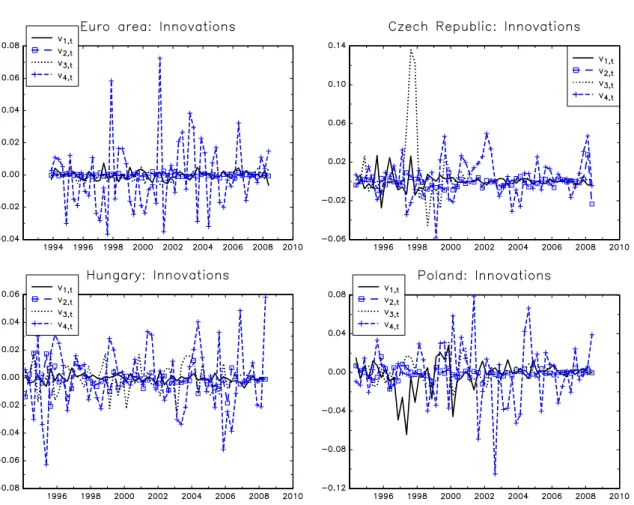
Hence, for these two countries the estimate can be regarded as quasi maximum likelihood estimates. Table 2 shows that autocorrelation of innovations is generally not a problem. The major exception is the third innovation of the Czech Republic and the first innovation of Hungary, which have highly significant Box-Pierce statistics. The third innovation of the Czech Republic also has largest Jearque-Bera statistic. As it can be seen from Figure 4, it is likely due to the huge innovation of the interest rate equation in 1997 when the Czech koruna
11 To completely get rid of non-zero means, we removed the mean separately from the left and right hand side variables. For example, when the lag length is two, the first variable and its lags were mean-removed as:
) 2
~ (
3 1, ,
1 ,
1 y
y Ty t t T , ~ 1 ( 2)
2 1, 1
, 1 1 ,
1 y
y Ty t t T , and
) 2
~ 2 (
1 1, 2
, 1 2 ,
1 y
y Ty t t T , where T denotes the number of observations before taking lags.
was hit by a speculative attack and interest rates rose sharply. Consequently, for the euro- area and Hungary the innovations well satisfy the key requirements needed for maximum likelihood estimation, while some of them are violated in the cases of the Czech Republic and Poland. This finding may be related to our result that estimations for the euro area and Hungary proved to be rather robust to the selection of the lag length, as different lag lengths did not alter much the shape of the impulse response functions. For Poland and the Czech Republic, however, the shapes of the impulse response functions differed somewhat when shorter lags were used, although the departures from normality and no-autocorrelation were also more serious with shorter lags.
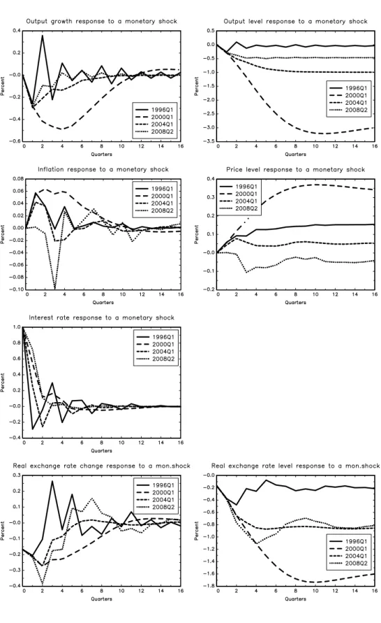
Due to the time varying parameters, impulse response functions also change from quarter to quarter. In order to conserve space and to enhance the discussion of our results, we show impulse response functions for four different dates of our sample, namely, for 1996Q1, 2000Q1, 2004Q1 and 2008Q2 in Figures 5, 6, 7 and 8.12
Figure 5 indicates that the output response to a monetary shock has declined in time in the euro area. This finding is in line with the findings of both Ciccarelli and Rebucci (2006) and Boivin, Giannoni and Mojon (2008). According to our calculations, while a 1 percentage point monetary shock lowered the long-run level of output by about 1.1 percent in 1996, this effect decreased monotonously in time to around -0.7 percent in 2008. For prices we got the so called price puzzle result, that is, prices increase after a monetary contraction,13 although this effect declined in time somewhat. The responses of the interest rate and the real exchange rate did not change much in time, suggesting that structural changes occurred mostly in the real economy.
Czech impulse responses in 1996Q1 were quite erratic, but became smoother later (Figure 6). It is noticeable that the real exchange rate did not respond to monetary shocks in 1996Q1, when the exchange rate was indeed fixed (see Section 0), but responded in later years when the exchange rate was floating. Among the dates shown in Figure 6, the largest responses can be observed in 2000Q1 on all variables, while the effects declined since then.
The price-puzzle finding, that characterized the results up to 2004, has disappeared by
12 The impulse responses were calculated on the basis of the time-varying parameters derived from the Kalman-smoother.
13 The price puzzle result is a general finding of many monetary VARs. The standard approach to get rid of this result, following a suggestion by Sims (1992), was to include commodity prices in the VAR as an indicator of future inflation. Hanson (2004), however, argues that the ability of commodity prices to mitigate the price puzzle may be due to an information channel – commodity prices respond more quickly than aggregate goods prices to future inflationary pressures – rather than serving as a proxy for marginal costs. We did not experiment with the inclusion of commodity prices or other approaches to get rid of the price puzzle because such extensions could further boost the number of time varying parameters to be estimated.
2008.14 Hence, all impulse responses change in time for the Czech Republic underlining the need for time-varying parameter analysis.
In Hungary monetary disturbances had only a tiny effect on output in the period 1996- 2004, while the effects increased somewhat by 2008 (Figure 7), but still the lowest among the countries studied as we will discuss later. The price-puzzle was a strong feature of the results in 1996 but it largely diminished in later years. The real exchange rate depreciated after a monetary shock, but the magnitude of the depreciation declined sharply by 2008.
Monetary policy became more effective in Poland as it is shown by Figure 8. The long run effect of a 1 percentage point monetary shock has increased from around -0.15 percent in 1996 and 2000 to around -0.65 percent by 2008. Parallel with this development, the otherwise negligible price puzzle in 1996 has diminished and our results indicate that a monetary shock had a sizable downward effect on prices in 2004 and 2008. It is also interesting to note that while the real exchange rate did not respond much to a monetary shock in 1996Q1 and had a small response in 2000Q1, the effect became sizable in 2004Q1 and 2008Q2. These results are in line with the evolution of the exchange rate regime described in Section 0, since the exchange rate was tightly managed in 1996 and gradually made flexible until April 2000 when a free floating was introduced.
Consequently, output response became weaker in the euro area and stronger in Hungary and Poland monotonously in time, while the time profile of change is not monotonous in the Czech Republic (though, the effect was stronger in 2008 than in 1996).
Figure 9 compares output responses in each of the three NMS with that of the euro area at the last observation of our sample, normalized, again, to a 1 percentage point monetary shock. In the three NMS, monetary policy is least effective in Hungary and most effective in Poland, while its effect in the Czech Republic is in between. The strength of the Polish response is comparable to that of the euro area. However, the time profile of the response is somewhat different for Poland and the euro area, since the long run effect is practically reached in one year for Poland, while the response of the euro area is more sluggish and the long run effect is reached at around two and a half years after the shock.
14 Using fixed parameter models for the sample period 1998-2006, Borys and Horváth (2008) do not find a price puzzle for the Czech Republic.
6. DISCUSSION
We suggest three possible explanations for these results: the credibility of monetary policy, openness, and the share of foreign currency loans.
As discussed in Section 2, Hungarian monetary policy adopted a crawling peg regime from 1995 to 2001. The approach of the central bank was to tightly manage the exchange rate in order to gradually decrease inflation without risking large trade imbalances, which was, by the way, a rather successful strategy for achieving these goals.15 While the widening of the band and the shift to inflation targeting in 2001 indicated a change in policy preferences, the tiny devaluation of the wide band in 2003 was a sign of a possible return to the former regime, largely weakening the credibility of the claim that pure inflation targeting is done.
Largely as a consequence of policy preferences, inflation was higher in Hungary than both in the Czech Republic and Poland in every year between 1995 and 2008. These factors could have contributed to the low credibility of central bank policy might, which might result in the low market response to monetary actions. The finding that response increased somewhat by 2008 (Figure 7) could indicate that the credibility of monetary policy has increased somewhat by 2008. By learning from the consequences of the 2003 exchange rate band devaluation central bank communication and actions were more focused on inflation.
Poland, on the other hand, adopted a very tight monetary policy even in an economic downturn.16 This could have contributed to the high credibility of monetary actions: market participants learned that policy was strict and resolute. Credibility of Czech monetary policy could have been in between of Hungary and Poland. The Czech central bank did not adopt such an aggressive monetary policy as Poland around the turn of the millennium but nonetheless it was quite successful since the average inflation was the lowest among the three new member states in our sample period.
Openness could also explain the differences: the Czech Republic and Hungary are rather open, while Poland is fairly closed. In more open economies output developments depend more on the foreign business cycle than in less open economies. This feature could mitigate the effects of domestic monetary policy. Furthermore, the share of foreign currency loans in total loans was much higher in Hungary, both for households and non-financial corporations (see Darvas and Szapáry, 2008), than in the Czech Republic and Poland, which highly constrains the effectiveness of domestic monetary policy.
15 See more details in Szapáry and Jakab (1998).
16 Regarding three month interbank interest rates and all items consumer price indices, the average real interest rate in Poland was 7.5 percent during 1997-2003, while it was 2.8 percent in Hungary and 3.3 percent in the Czech Republic.
7. SUMMARY
This paper studied the transmission of monetary policy in three new members states of the EU with structural time-varying coefficient VARs in comparison with that in the euro area. In line with the Lucas Critique, reduced-form models, like standard VARs, are not invariant to changes in policy regimes. Many of the new Member States have experienced changes in monetary policy regimes, which call for the use of a time-varying parameter analysis.
Furthermore, in addition to policy changes these countries went through substantial structural changes. More generally, since most of the empirical models, including VARs, are linear models, their parameters can change even if the underlying structural model has constant parameters but it is nonlinear.
Our results indicate that some parameters change significantly altering the shape of the impulse response functions. The response of output to a monetary shock has changed in the euro area as well as in the Czech Republic, Hungary and Poland. Output response became weaker in the euro area, well in line with the findings of Ciccarelli and Rebucci (2006) and Boivin, Giannoni and Mojon (2008). Output response became stronger in Hungary and Poland monotonously in time, while the time profile of change is not monotonous in the Czech Republic (though the effect was stronger in 2008 than in 1996). At the last observation of our sample, the second quarter of 2008, among the three countries studied, monetary policy was the most powerful in Poland and comparable in strength to that in the euro area (though with a different time profile) and was the least powerful in Hungary, while the strength of monetary policy in the Czech Republic lied in between. We explained these differences by the credibility of monetary policy, openness and the share of foreign currency loans: the effect of monetary policy on output is small in countries that are highly open, have a high share of foreign currency loans, and whose central bank is regarded less credible.
Figure 1 Nominal Exchange Rate of the Czech Koruna
1 January 1995 to 30 June 2008
2.55 2.60 2.65 2.70 2.75 2.80 2.85 2.90 2.95 3.00 3.05 3.10 3.15 3.20
01.95 01.96 01.97 01.98 01.99 01.00 01.01 01.02 01.03 01.04 01.05 01.06 01.07 01.08
logarithm of koruna per basket (inverted scale)
2.55 2.60 2.65 2.70 2.75 2.80 2.85 2.90 2.95 3.00 3.05 3.10 3.15 3.20
Source: Updated from Darvas and Szapáry (2000).
Notes: Basket used prior to May 1997: 65% DEM - 35% USD. For better comparison we use both the compositon of the basket and the euro for the floating period.
Koruna let to float Width of the band:
+/- 7,5 %
euro basket
Width of the band:
+/- 0,5 %
Figure 2 Nominal Exchange Rate of the Hungarian Forint
1 January 1994 to 30 June 2008
4.5
4.6 4.7
4.8
4.9
5.0
5.1 5.2
5.3
5.4
5.5 5.6
94-01 95-01 96-01 97-01 98-02 99-02 00-02 01-02 02-02 03-02 04-02 05-01 06-01 07-01 08-01
logarithm of forint per basket (inverted scale)
4.5
4.6 4.7
4.8
4.9
5.0
5.1 5.2
5.3
5.4
5.5 5.6
Source: Updated from Darvas and Szapáry (2000)
Notes: Composition of the basket: 50% DM+50% USD for August 1993 - May 1994; 70% ECU+30% USD for May 1994 - December 1996; 70%
DEM+30% USD for January 1997 - December 1998; 70% EUR+30% USD for January - December 1999; 100% EUR since 2000.
Width of the band:
+/- 2.25%
Width of the band:
+/- 1.25%
Width of the band:
+/- 0.5%
Width of the band:
+/- 15%
Figure 3 Nominal Exchange Rate of the Polish Zloty
1 February 1995 to 30 June 2008
0.7
0.8
0.9
1.0
1.1
1.2
1.3
02-95 02-96 02-97 02-98 02-99 02-00 02-01 02-02 02-03 02-04 02-05 02-06 02-07 02-08
logarithm of zloty per basket (inverted scale)
0.7
0.8
0.9
1.0
1.1
1.2
1.3 width of
the band:
+/- 15%
width of the band:
+/- 10%
width of the band:
+/- 12.5%
Source: Updated from Darvas and Szapáry (2000).
Note: Composition of the basket prior to 1999: 45% USD, 35% DM, 10% GBP, 5% FRF, 5% CHF; since 1999: 55% EUR , 45% USD. Zloty was let to float in April 2000. For better comparison we use both the compositon of the last basket and the euro for the floating period.
width of the band:
+/- 7%
euro basket
Zloty let to float
Figure 4 Innovations
Note. The four series shown are innovations to the equations of output growth, inflation, interest rate and real exchange rate changes, respectively.
Figure 5 Euro area: Impulse response functions at different dates
Figure 6 Czech Republic: Impulse response functions at different dates
Figure 7 Hungary: Impulse response functions at different dates
Figure 8 Poland: Impulse response functions at different dates
Figure 9 Output growth and level response to a monetary shock at 2008Q2
Note: the size of the shock is 1 percentage point.
Table 1 Jarque-Bera normality test for innovations
Euro area Czech Rep. Hungary Poland
v1,t 0.5 57.4 0.8 67.9
(0.785) (0.000) (0.678) (0.000)
v2,t 0.9 88.1 4.3 14.5
(0.627) (0.000) (0.114) (0.001)
v3,t 3.4 521.0 1.2 5.5
(0.184) (0.000) (0.561) (0.063)
v4,t 11.1 1.1 0.0 4.0
(0.004) (0.588) (0.984) (0.136)
Note. P-values in parentheses.
Table 2 Box-Pierce autocorrelation test for innovations
Euro area Czech Rep. Hungary Poland
v1,t 4.8 8.6 24.8 10.6
(0.566) (0.197) (0.001) (0.101)
v2,t 4.9 4.0 5.3 4.5
(0.562) (0.683) (0.502) (0.607)
v3,t 6.4 22.5 10.2 9.9
(0.382) (0.001) (0.118) (0.127)
v4,t 12.3 2.8 9.1 1.2
(0.055) (0.839) (0.167) (0.977)
Note. P-values in parentheses.
REFERENCES
Angeloni, Ignazio, Anil K. Kashyap and Benoît Mojon, eds. 2003. Monetary Policy Transmission in the Euro Area: A Study by the Eurosystem Monetary Transmission Network. Cambridge University Press.
Boivin, Jean, Marc P. Giannoni and Benoît Mojon, 2008. How Has the Euro Changed the Monetary Transmission? NBER Working Papers No. 14190.
Borys, Magdalena Morgese and Roman Horváth, 2008. The Effects of Monetary Policy in the Czech Republic: An Empirical Study. Working Paper 4/2008, Czech National Bank.
Canova, Fabio and Gianni De Nicolo. 2002. Monetary Disturbances Matter for Business Cycles Fluctuations in the G7. Journal of Monetary Economics 49. 1131–1159.
Canova, Fabio and Luca Gambetti. 2006. Structural Changes in the US Economy. Bad Luck or Bad Policy? CEPR Discussion Paper No. 5457.
Christiano, Lawrence J., Martin Eichenbaum, and Charles L. Evans. 1999. Monetary Policy Shocks: What Have We Learned and to What End? In: Handbook of Macroeconomics, Vol. 1A. John B. Taylor and Michael Woodford (eds.). New York: Elsevier Science. 65–
148.
Ciccarelli, Matteo and Alessandro Rebucci. 2006. Has the Transmission Mechanism of European Monetary Policy Changed in the Run-Up to EMU? European Economic Review 50, 737-776.
Cogley, Timothy and Thomas J. Sargent. 2005. Drifts and Volatilities: Monetary Policies and Outcomes in the Post WWII US. Review of Economic Dynamics 8. 262–302.
Darvas, Zsolt and György Szapáry, 2000. Financial Contagion in Five Small Open Economies: Does the Exchange Rate Regime Really Matter? International Finance 3(1), 25-51.
Darvas, Zsolt and György Szapáry, 2008. Euro Area Enlargement and Euro Adoption Strategies. European Economy - Economic Papers 304, DG-ECFIN, European Commission, Brussels. Forthcoming in: Buti, Marco, Servaas Deroose, Vitor Gaspar and João Nogueira Martins (eds.): Euro-The First Decade, Cambridge University Press.
Darvas, Zsolt, 2001. Exchange rate pass-through and real exchange rate in EU candidate countries. Deutsche Bundesbank Discussion Paper No. 10/2001.
Darvas, Zsolt, 2008. Sign restrictions are more robust than long-run restrictions in structural VARs. To appear as a Deutsche Bundesbank Discussion Paper.
Égert, Balázs and Ronald MacDonald, 2008. Monetary Transmission Mechanism in Central and Eastern Europe: Surveying the Surveyable. Forthcoming in Journal of Economic Surveys.
Faust, Jon and Eric M. Leeper 1997. When Do Long-Run Identifying Restrictions Give Reliable Results? Journal of Business and Economic Statistics, 15(3), 345–353.
Fry, Renee and Adrian Pagan, 2007. Some Issues in Using Sign Restrictions for Identifying Structural VARs. NCER Working Paper No. 14.
Granger, Clive W.J., 2008. Non-Linear Models: Where Do We Go Next – Time Varying Parameter Models? Studies in Nonlinear Dynamics and Econometrics 12(3), The Berkeley Electronic Press.
Hamilton, James D., 1994. Time Series Analysis. Princeton University Press.
Hanson, Michael S., 2004. The “Price-Puzzle” Reconsidered. Journal of Monetary Economics 51, 138-1413.
He, Changli, Timo Teräsvirta and Andres González, forthcoming. Testing parameter constancy in stationary vector autoregressive models against continuous change.
Forthcoming in Econometric Reviews.
Szapáry, György and Zoltán M. Jakab. 1998. Exchange Rate Policy in Transition Economies: The Case of Hungary. Journal of Comparative Economics 26(4) 691-717.
Peersman, Gert, 2005. What Caused the Early Millennium Slowdown? Evidence Based on Vector Autoregressions. Journal of Applied Econometrics 20, 185-207.
Primiceri, Giorgio E. 2005. Time Varying Structural Vector Autoregressions and Monetary Policy. Review of Economic Studies 72(3), 821-852.
Sims, Christopher A. 1992. Interpreting Macroeconomic Time Series Facts: The Effects of Monetary Policy. European Economic Review 36(5), 975-1000.
Sims, Christopher A. and Tao Zha, 2006. Were there regime switches in US monetary policy? American Economic Review 96(1), 54-81.
Stock, James H. and Mark W. Watson, 2005. Understanding Changes In International Business Cycle Dynamics. Journal of the European Economic Association 3(5), 968- 1006.
Uhlig, Harald, 2005. What are the Effects of Monetary Policy: Results from an Agnostic Identification Approach. Journal of Monetary Economics 52, 381-419.
Várpalotai, Viktor, 2003. Numerical Method for Estimating GDP Data for Hungary.
Magyar Nemzeti Bank Working Paper No. 2003/2.
Discussion Papers published since 2008
2008
CSERES-GERGELY Zsombor - MOLNÁR György: Háztartási fogyasztói magatartás és jólét Magyarországon. Kísérlet egy modell adaptációjára. MT-DP.2008/1
JUHÁSZ Anikó – KÜRTI Andrea – SERES Antal – STAUDER Márta: A kereskedelem koncentrációjának hatása a kisárutermelésre és a zöldség-gyümölcs kisárutermelők alkalmazkodása. Helyzetelemzés. MT-DP. 2008/2
Ákos VALENTINYI – Berthold HERRENDORF: Measuring Factor Income Shares at the Sectoral Level. MT-DP.2008/3
Pál VALENTINY: Energy services at local and national level in the transition period in Hungary. MT-DP.2008/4
András SIMONOVITS: Underreported Earnings and Old-Age Pension: An Elementary Model. MT-DP.2008/5
Max GILLMAN – Michal KEJAK: Tax Evasion and Growth: a Banking Approach.
MT-DP.2008/6
LACKÓ Mária – SEMJÉN András: Rejtett gazdaság, rejtett foglalkoztatás és a csökkentésükre irányuló kormányzati politikák - irodalmi áttekintés. MT-DP.
2008/7
LACKÓ Mária: Az adóráták és a korrupció hatása az adóbevételekre - nemzetközi összehasonlítás (OECD országok, 2000-2004). MT-DP. 2008/8
SEMJÉN András – TÓTH István János – FAZEKAS Mihály: Az EVA tapasztalatai vállalkozói interjúk alapján. MT-DP. 2008/9
SEMJÉN András – TÓTH István János – FAZEKAS Mihály: Alkalmi munkavállalói könyves foglalkoztatás munkaadói és munkavállói interjúk tükrében. MT-DP.
2008/10
SEMJÉN András – TÓTH István János – MAKÓ Ágnes: Az alkalmi munkavállalói könyvvel történő foglalkoztatás jellemzői. Egy 2008. áprilisi kérdőíves munkavállalói adatfelvétel eredményei. MT-DP. 2008/11
FAZEKAS Mihály: A rejtett gazdaságból való kilépés dilemmái
Esettanulmány - budapesti futárszolgálatok, 2006-2008. MT-DP. 2008/12
SEMJÉN András – TÓTH István János – MEDGYESI Márton – CZIBIK Ágnes:
Adócsalás és korrupció: lakossági érintettség és elfogadottság. MT-DP. 2008/13 BÍRÓ Anikó - VINCZE János: A gazdaság fehérítése: büntetés és ösztönzés.
Költségek és hasznok egy modellszámítás tükrében. MT-DP. 2008/14
Imre FERTŐ - Károly Attila SOÓS: Marginal Intra-Industry Trade and Adjustment Costs - A Hungarian-Polish Comparison. MT-DP. 2008/15
Imre FERTŐ - Károly Attila SOÓS: Duration of trade of former communist countries at the EU. MT-DP. 2008/16
FERTŐ Imre: A magyar agrárexport kereskedelmi előnyei és versenyképessége az EU piacán. MT-DP. 2008/17
Zsolt BEDŐ - Éva OZSVALD: Codes of Good Governance in Hungary. MT-DP.
2008/18
DARVAS Zsolt - SZAPÁRY György: Az euróövezet bővítése és euróbevezetési stratégiák. MT-DP. 2008/19
László Á. KÓCZY: Strategic Power Indices: Quarrelling in Coalitions. MT-DP.
2008/20
Sarolta LACZÓ: Riskiness, Risk Aversion, and Risk Sharing: Cooperation in a Dynamic Insurance Game. MT-DP. 2008/21
Zsolt DARVAS: Leveraged Carry Trade Portfolios. MT-DP. 2008/22
KARSAI Judit: "Az aranykor vége" - A kockázati- és magántőke-ágazat fejlődése Közép- és Kelet-Európában. MT-DP. 2008/23
Zsolt DARVAS - György SZAPÁRY: Euro Area Enlargement and Euro Adoption Strategies. MT-DP. 2008/24
Helmuts ĀZACIS - Max GILLMAN: Flat Tax Reform: The Baltics 2000 – 2007. MT- DP. 2008/25
Ádám SZENTPÉTERI - Álmos TELEGDY: Political Selection of Firms into Privatization Programs. Evidence from Romanian Comprehensive Data. MT-DP.
2008/26
DARVAS Zsolt - SZAPÁRY György: Az új EU-tagországok megfelelése az optimális valutaövezet kritériumainak. MT-DP. 2008/27
CSATÓ Katalin: Megjegyzések Navratil Ákos elmélettörténetéhez. MT-DP. 2008/28
2009
Judit KARSAI: The End of the Golden Age - The Developments of the Venture Capital and Private Equity Industry in Central and Eastern Europe. MT-DP.
2009/1
András SIMONOVITS: When and How to Subsidize Tax-Favored Retirement Accounts? MT-DP.2009/2
Mária CSANÁDI: The "Chinese style reforms" and the Hungarian "Goulash Communism". MT-DP. 2009/3
Mária CSANÁDI: The Metamorphosis of the Communist Party:
from Entity to System and from System towards an Entity. MT-DP. 2009/4
Mária CSANÁDI – Hairong LAI – Ferenc GYURIS: Global Crisis and its Implications on the Political Transformation in China. MT-DP. 2009/5
DARVAS Zsolt - SZAPÁRY György: Árszínvonal-konvergencia az új EU tagországokban: egy panel-regressziós modell eredményei. MT-DP. 2009/6
KÜRTI Andrea - KOZAK Anita - SERES Antal - SZABÓ Márton: Mezőgazdasági kisárutermelők nagy kereskedelmi láncooknak történő beszállítása a nagyvevői igények alapján a zöldség-gyümölcs ágazatban. MT-DP.2009/7
András SIMONOVITS: Hungarian Pension System and its Reform. MT-DP.2009/8 Balázs MURAKÖZY - Gábor BÉKÉS: Temporary Trade. MT-DP. 2009/9
Alan AHEARNE - Herbert BRÜCKER - Zsolt DARVAS - Jakob von WEIZSÄCKER:
Cyclical Dimensions of Labour Mobility after EU Enlargement. MT-DP. 2009/10 Max GILLMAN - Michal KEJAK: Inflation, Investment and Growth: a Money and
Banking Approach. MT-DP. 2009/11
Max GILLMAN - Mark N. HARRIS: The Effect of Inflation on Growth: Evidence from a Panel of Transition Countries. MT-DP. 2009/12
Discussion Papers are available at the website of Institute of Economics Hungarian Academy of Sciences: http://econ.core.hu