I am grateful to Csaba H˝os that I was able to learn the basic theory of the piecewise smooth dynamical systems. This research was motivated by the recognition of the interaction of the effect of these phenomena on the system dynamics.
Friction phenomena and models
It was concluded that the frictional force is proportional to the normal load, but it is independent of the apparent contact area and acts in the opposite direction of the motion. However, it was later shown that the frictional force depends on the true contact area [6].
Friction problems in mechatronics
To overcome this problem, an extension of the Dahl model was constructed, in the form of the so-called LuGre friction model [26]. However, in these studies, the effect of the dry friction is considered as a stabilizing effect and is neglected.
State of the art
Reference [51] presents design tools and methods for discretely controlled robots, and [52–54] focuses on the analytical investigation of digital force control dynamics. Therefore, the main purpose of the research summarized in this dissertation is to investigate the effects of friction on the dynamics of mechanical systems with discrete time control.
Thesis outline
At the end of this chapter, the stability properties of the sampled-data sliding-oscillator model are further analyzed. This continuous-time system model is also used to analyze the stability properties of the sliding oscillator model with sampled data.
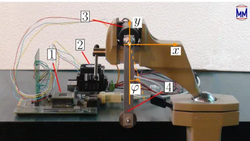
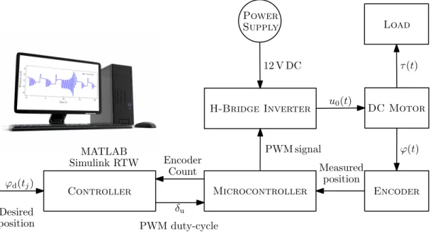
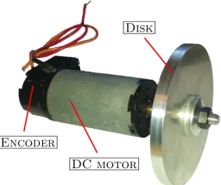
Modeling of the experimental setup
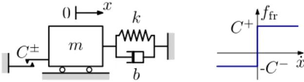
Model of dry friction
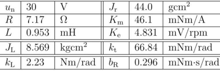
According to the Coulomb friction model, it is assumed that the magnitudes of the static and the kinetic friction torque are equal, the friction torque is given in the form. where τC indicates the magnitude of the kinetic or Coulomb frictional torque. The magnitude of the Coulomb friction torqueτC can initially be approximated as τC = Kmi0 = 1.4844 mNm, where i0 is the no-load current [61].
Discrete-time control realization
At the beginning of the time interval [tj−1, tj), at instant tj−1, the sampled position data is φ(tj−1). Based on these, the control torque τu =−kpϕ(tj−1) can also be expressed as τu(t) = Km. 2.18) It turns out that the required value of the duty cycle is.

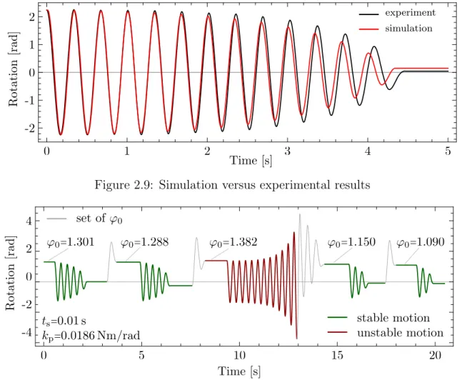
Validating experimental results
The value of δmax is limited by the settings (e.g. selected PWM frequency) of the microcontroller and the efficiency of the H-bridge converter. The achievable maximum value of δmax is 800 due to the selected 20 kHz PWM frequency in the applied microcontroller and due to the efficiency of the H-bridge converter it is limited to δmax = 794.
Simplest representative model
On this basis it can be concluded that the simulation results, in which the effect of the additional unit delay is not taken into account, and the experimental results initially correspond very well. When comparing simulations with and without a unit delay, it can be seen that the effect of delay is negligible in the case of the current parameter setting.
Piecewise analytical simulation
Piecewise analytical solution
By means of these bits of solutions and using the time-discrete proportional controller, fu = −kpxj, the following non-homogeneous discrete map can be created.
Evolution of the discrete states
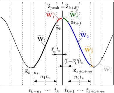
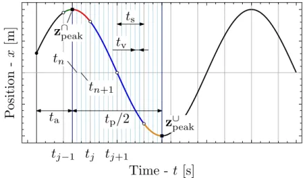
Depending on the direction of the transition, the resulting vibration peaks can be local maxima zpeak∩ or local minima zpeak∪. Using the last simulated states before zk velocity reversal occurs, the sampling time fraction and also the vibration peak magnitude can be determined using Eq. Taking the sampling time constant, the state variables at the end of the sampling period can be defined as.
New Results
A closed form discrete simulator is proposed for solving the initial value problem of the sample data sliding oscillator. Consider the discrete-time model of the sample data sliding oscillator in the form zj+1 = W(ts)zj −w(ts) sgn (˙x(t)) with. In addition, tj denotes the jth sampling instant, ts is the sampling time and x(tj) denotes the sampled general coordinate at the beginning of the jth time interval.
Stability analysis by neglecting friction
By means of these solution parts, the following non-homogeneous discrete map can be created. in the linear map in Eq. 3.7), results in the characteristic equation. Note that the coefficients of the characteristic polynomial, here, were directly determined using the defining identity of the matrix sum published in [65]. It follows from [64] that the system is asymptotically stable if and only if the magnitudes of the complex eigenvalues zi = exp(skT) of the discrete state matrix Wc are smaller than 1, i.e.
Energetic stability analysis
Effective viscous damping
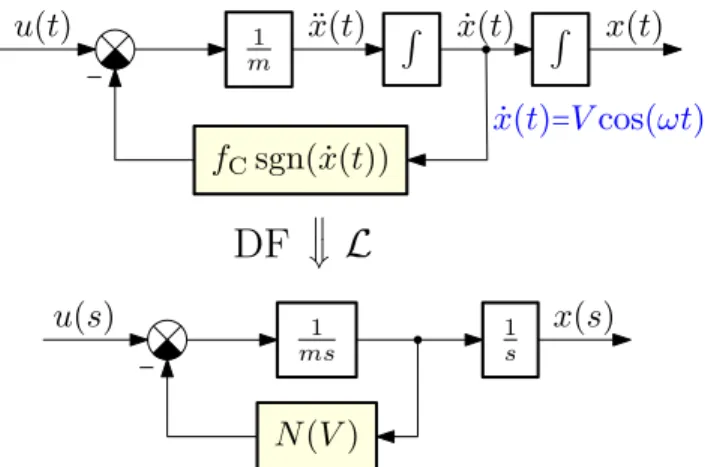
Focusing on the approximation of the effect of dry friction, the equation of motion is considered in the form. When the motion is initiated with the following conditions x(0) =x0 = 0 and ˙x(0) = v0 >0, then the amplitude of the velocity function becomes V =v0. In order to understand the effect of viscous damping on the stability of the sampled data damped oscillator, using the control law of the discrete-time proportional controller u=−kpx(tj), the following model is investigated.
Passivity condition with effective viscous damping
2 , (3.29), where U is the potential energy, which represents the stored energy in a fictitious physical spring realized by the discrete-time proportional controller, while the second term with kp on the right-hand side of Eq. 3.30) represents the energy instillation effect of zero-order hold [70]. Using the following approximation of the velocity. the remaining integral in Eq. 3.30) can be approximately determined as. Thus, the left side of the equation above must be negative, and therefore the following inequality must be satisfied. 3.34) It is clear, the expression (xj+1−xj)2 is always positive, therefore the total mechanical energy decreases when.
Vibration decay and stability analysis
Critical initial conditions
2.3, a new non-homogeneous mapping can be derived that has the same form as before, but ts is replaced with tv. Due to this special choice of TV, a mapping can be built between the vibration peaks. Based on this, it can be concluded that making n steps with the virtual sampling time tv gives the same result as making π/ϑ steps with the original sampling time ts.
Special subset of system parameters
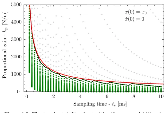
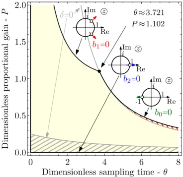
3.2, the stability limit is determined by Eq. 3.54) and is represented as a black solid line in the figure. As can be seen in the region of longer sampling times, the zigzag limit touches the limit of quasi-analytical stability. On the other hand, for shorter zigzag sampling times, the stability limit converges to the quasi-analytical stability limit.
New Results
Therefore, negative damping in this parameter domain can be used to characterize the motion of the system, because β > 0 and the dominant vibrational frequency α0 is the damped natural angular frequency. where ω0 and ζ0 are respectively the dominant natural frequency and the dominant damping ratio, which characterize the dynamics of the time-discrete system when the higher harmonics are negligible. By comparing the coefficients of Eq. 4.5), the dominant natural angular frequency and the dominant damping ratio can be expressed with the parameters of the discrete-time system as It can be concluded that the effect of sampling, which neglects the higher harmonics, results in a continuous-time damped oscillator model where the viscous damping term is negative.
Dynamic analysis of the continuous-time damped- oscillator with dry friction
- Motion induced by initial condition
- Piecewise smooth analysis
- Limit cycles and vibrations
- Relationship between the initial conditions
In this case, the first half-period of the motion takes place with negative velocity, so the solution of Eq. 4.8) until the first velocity reversal can be obtained as. Similar to the method presented above, the constants Cn can be determined for the nth half-period of the motion axis. 4.15). The main purpose of this section is the derivation of the condition for critical initial position at zero initial velocity, when unstable limit cycle can occur.
Application to discrete-time position control
These can be used to determine the first local minimax∪peak or local maximax∩peak and using the critical initial positions in Eq. Furthermore, when both initial conditions are nonzero, using the method written above, the critical initial conditions can be determined in a simple additional step. If the sum of the magnitudes of this peak and the given initial position equals the critical initial position, then a limit cycle exists. In addition to sampling time and control gain, a third parameter that determines the critical initial positions is the generalized friction force.
New Results
The model investigated in this chapter takes into account both viscous damping and dry friction. In robotic systems, the power losses that play an important role in dynamics generally consist of a viscous damping and a Coulomb friction term [73]. The extended friction oscillator model with sampled data and viscous damping can be written as follows.
Stability analysis without friction
With this, the dimensionless sampling instant is Tj = jβts = jθ, where θ denotes the dimensionless sampling period, and the sampled control input is x(Tj) =xj. The corresponding stable domain of control parameters is illustrated in the plane of the dimensionless sampling time θ and the dimensionless proportional gain P in Fig. In the usual yellow region, the characteristic multipliers show z1,2 ∈C with Im(z1,2)6= 0 and the system shows similar oscillations as an underdamped second-order system.
Combined effect of dry friction and viscous damp- inging
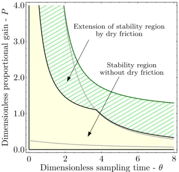
When the resultant of this negative damping and the physical viscous damping is negative, there will be an unstable limit cycle, and its magnitude is given by Eq. Based on this expression, the region of attraction of the desired position xd = 0 is determined by the stability criterion. The consideration of dry friction results in a significant expansion of the stable operating region compared to the frictionless model.
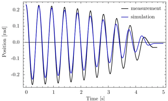
Verification of results
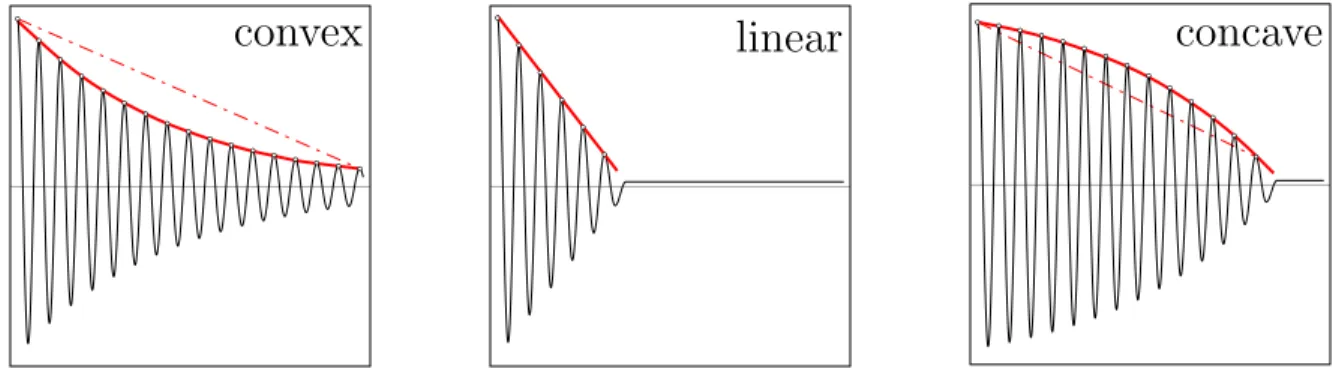
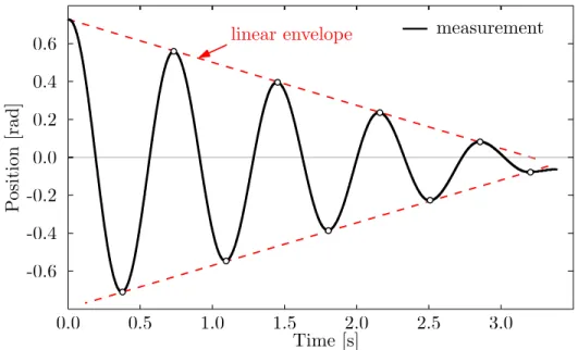
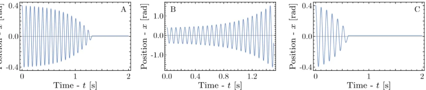
The other two simulation results, at point B and C, show that the system is unstable and stable close to the stability limit, respectively. Typical dynamic behavior when the analyzed system is stable and damped by both viscous damping and Coulomb friction is shown in Fig. It can be concluded that when Coulomb friction stabilizes the otherwise unstable motion, the damped vibrations have concave envelope.
New Results
Theorem: The determinant of the sum of two real element, two-by-two matrices can be expressed in the form. Because the left-hand side is equal to the right-hand side statement in Eq. Application: This theorem can be used during the derivation of the characteristic polynomial with the following substitutions A =−zI and B =W.
Experimental comparison of five friction models on the same testbed of the microstick slip motion system.Mechanical Sciences. In Proceedings of the IEEE International Conference on Robotics and Automation, volume 2, pages Kohala Coast, HI, USA, 1999.