Aerodynamic Shape Optimization with the Adjoint Method

Atualmente, esse trabalho é realizado por engenheiros com muitos anos de experiência, que utilizam seu amplo conhecimento em aerodinâmica de aeronaves. No entanto, este trabalho é feito manualmente e por tentativa e erro, o que se torna especialmente desafiador com geometrias e aerodinâmicas complexas. Ou seja, a otimização da forma aerodinâmica com o método adjunto oferece muitas vantagens sobre outras técnicas.

Esta técnica, juntamente com outras, será estudada e aplicada na otimização de um aerofólio transônico e de uma asa de uma aeronave Airbus de longo curso.

Nomenclature

Glossary

Introduction

Motivation
Topic Overview
Objectives
Outline

These determine the successive designs based on the gradient of the objective function with respect to the design variables. The adjoint method presents itself as an answer to this problem and has several advantages over such conventional gradient calculation methods. An optimization of a transonic airfoil and of a long-range aircraft wing with a gradient-based algorithm, aided by the additional gradient calculation method, will be studied.

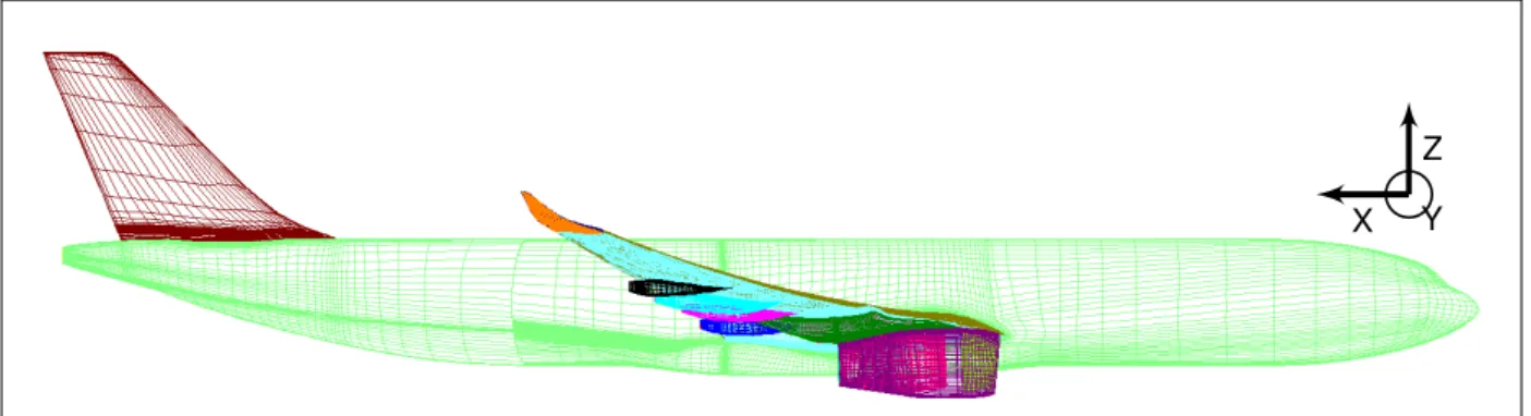
Finally, the fourth part is devoted to a real three-dimensional case of the wing of a long-range aircraft designed by Airbus.

Aerodynamic Shape Optimization

Aerodynamics

Navier-Stokes Equations
Reynolds Averaged Navier-Stokes Equations (RANS)
Compressible Reynolds Averaged Navier-Stokes Equations
Spalart-Allmaras Turbulence Model
Aerodynamic Dimensionless Coefficients

Pressure Coefficient
Friction Coefficient
Drag Coefficient
Lift Coefficient
Pitching Moment Coefficient

2.8), where Re is called the Reynolds number defined in Eq. 2.9) ρref, Uref and µref are usually taken at infinite (undisturbed field) and Lref is often the aerofoil/wing (possibly mean aerodynamic) chord. The friction coefficient (2.14) is the local wall shear stress τw, non-dimensionalized by the free-stream dynamic pressure. DragDis defined as the force parallel to the free-stream velocity U~∞, which non-dimensionalized by the free-stream dynamic pressure times a reference surface area Sref yields the drag coefficient Eq. 2.15). However, because spurious viscous or wave resistance can be generated inVsp≡V \(VV +VW) using the numerical scheme used to solve the equations, outside the volumes VV and VW where the production of viscous or wave resistance is physically justified, will near-field/far-field balance become equal. LiftLis defined as the force perpendicular to the freestream velocity U~∞, which non-dimensionalized by the freestream dynamic pressure times a reference surface area Sref yields the lift coefficient Eq. 2.21).

In a similar manner to the previous aerodynamic coefficients, the pitching moment coefficient is defined in Eq. 2.23), where Lref is the reference length, usually (preferably the mean aerodynamic) chord.

Shape

Optimization

Problem Definition
Gradient-based optimization

Gradient computation by finite differences
Gradient computation by the adjoint method
Karush–Kuhn–Tucker (KKT) conditions
Sequential Least Squares Programming (SLSQP)

Design of Experiments (DOE)

The basic information in all gradient-based algorithms is the sensitivity or gradient of the cost function with respect to the design variables D. Based on this gradient, the optimizer (the optimization algorithm) decides where to go in the design space. The gradient (2.25) can be calculated by forward Eq. 2.26b) finite differences, which are first-order methods. 2.26b), we obtain the centered finite difference Eq. Therefore, the calculation of the gradient Eq. 2.25) requires|D|+ 1flow solutions (CFD evaluation) for first-order methods - onef(D+ ∆D)for each∆Di the direction of each design variable plus f(D).

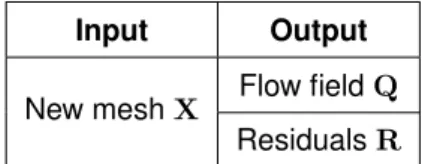
In both cases, the cost of gradient computation is directly proportional to the number of design variables |D|. The finite-difference gradient calculation error as a function of the step ∆D is shown in the figure. Consider the vector of discretized residual equations for the Navier-Stokes equations R = R(Q,X) and its stationary solution of the form R(Q,X) = 0.

We define the Lagrangian function L given by Eq. 2.28), where Λ represents a vector of Lagrange multipliers or associated variables. meaning that if we compute the dDdL gradient, we also compute the dDdf gradient needed for the gradient-based optimization algorithm. 2.28) with respect to D and rearranging the terms gives the equation is computationally expensive as it requires many flux solutions proportional to |D|, as in Section 2.3.2.1. However, since Λ is essentially arbitrary, the multiplication factor is ∂Q. can be solved by Eq. 2.30), which is called the associated system of equations. The dDdL gradient is then given by Eq. 2.31) The term ∂X∂D represents the mesh sensitivity and is developed in Eq. This applies, for example, to the boundary constraints of the design space xi∈[li, ui]⇔xi−ui≤0∧li−xi≤0.

The Lagrangian of the problem is given by Eq. 2.36), where µ and λ are the Lagrange multipliers. The generalization of a Latin square to an arbitrary number of dimensions is called a Latin hypercube.

Analysis and Optimization Tools

Computational Fluid Dynamics

Mesh
Solver

WORMS Optimization Chain

Padge

Shape Matching
CAD to Mesh Link

VolDef
elsA

Target Lift

ZAPP/ZAPP-rev
elsA-reverse
VolDef-reverse
Padge-reverse
Optimizer

To be able to calculate the displacement δXs=Xs−X0s, the location of each point X0s. This is done by finding a tuple (u, v)i =F−1((X0s)i) for each mesh point of the initial surface mesh and supplying it with the new surface mapF(u, v) =F( D, u, v). This deformation is done by layers inside a cone that protrudes from the surface, with an exponential damping factor.

The target lift method works by varying the angle of attack until it finds an angle of attack for which the lift coefficient is equal to the target lift coefficient. When|(CL)target-CL(αn)| ≤, with a predefined tolerance, the iterative algorithm is stopped and a CFD simulation is performed for NStepEndstime final steps. ZAPP is a post-processing tool responsible for calculating the desired performance metricsfi (eg: CD, CL, etc.) and its inverse mode calculates their partial derivatives with respect to the grid nodes ∂f∂Xi and with respect to the variable flux vector ∂f ∂Qi.

The adjoint mode is then used to compute the full derivative of the function fi with respect to the positions of the mesh nodes (3.2). VolDef-reverse computes the derivative of the functions fi with respect to the surface mesh nodes. It calculates the partial derivative ∂X∂Xs and multiplies by the full derivative (3.2) calculated with elsA inverse, resulting in Eq.

Padge-reverse is responsible for the final step, which is the transformation of the derivative with respect to the surface mesh nodes, i.e. the "shape", into a derivative with respect to the design variables. The optimizer receives the gradient of the objective and constraint functions and decides the next set of design variable valuesD.

Post-processing

KKT Optimization Analysis
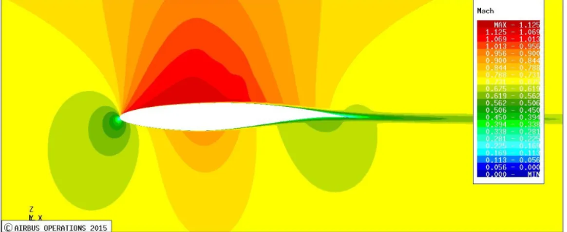
Flow visualization
FFD Aerodynamic Analysis

RAE2822 Airfoil Optimization

Test Case Definition

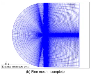
Mesh
Baseline Design

Problem Description

CT-Parameterization
Design Space
Optimization Problem

Unconstrained Optimization

Optimization Analysis
Aerodynamic and Geometry Analysis
Global Behavior

Constrained Optimization

Constrained Optimization Problem
Influence of ∆C lp and Optimization Analysis

Changing Adaptation C lp

Optimization Analysis

Conclusion

When the optimization is performed from a "baseline design", the latter is preferred, since 0 is used as the reference for the baseline. The corresponding normalized variable isx and the basis of the design space normalization is the linear transformation (4.1). The true gradient on the non-normalized design space points in the direction of the local minimum.

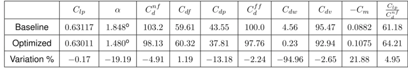
However, since the optimization and the gradient are calculated in the normalized design space, the x-component of the gradient on the non-normalized design space is multiplied by α2x = 4 and the y-component is not changed because. Each gradient component is multiplied by the corresponding scale factor of the variable α (not the same for all variables). The drag breakdown obtained from the far-field analysis of the optimized airfoil is given in Tbl.

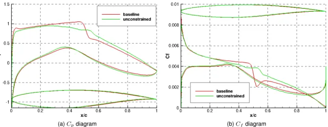
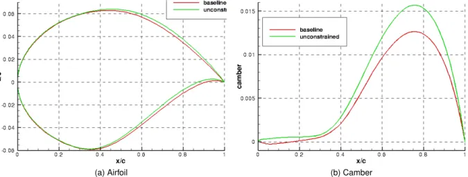
The gain inCdpis is very close to that calculated with the optimization values, validating the use of the "medium" mesh. The impact strength is clearly reduced when comparing Cp to the baseline design on the upper side at about 50% of the chord. Due to the adaptation shift phenomenon with the unconstrained optimization, a constraint must be imposed to keep the adaptation at Clp= 0.63(4.6).

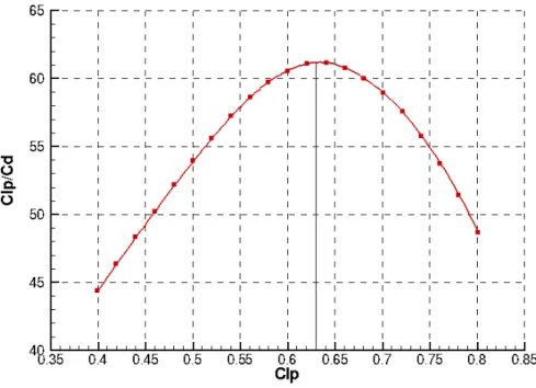
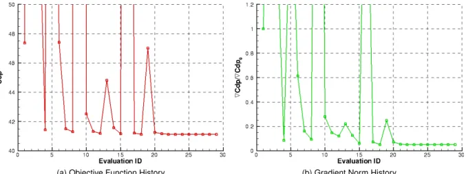
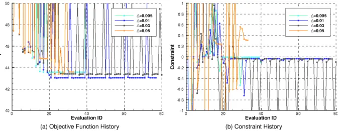
The history of both objective function and constraint is shown in fig. The∆ = 0.05 optimization completed very quickly in under thirty-five iterations—such a large step involves checking points far apart. On both the baseline and unconstrained optimized airfoils, camber is very small in the first 30% of the airfoil. The best gain of the objective function is obtained for Clp∗ = 0.63, which was discussed in Section 4.4.

The objective of the original optimization problem was set as optimizing the value of the maximum CClp.

Winglet Optimization

Test Case Definition

Mesh
Parameterization

Design of Experiments

Identification of problematic combinations of design variables values
Relation between the objective function and constraint
Design variable influence analysis

Baseline Solution
Adjoint Optimization

Starting from Baseline
Starting from DOE Designs

Optimized Database

Planform DOE
Optimized Solutions

Conclusion

The limits of the modification to the baseline for each design variable are given in Tbl. With such complex geometry and aerodynamics, exacerbated by the high number of design space dimensions, understanding the design space is difficult. As the number of dimensions of the design space grows larger, the number of points needed to have a significant sample grows exponentially.

A scatter plot of the objective function versus the constraint is shown in Fig. 5.2) is very unlikely, or conversely, the optimal is very likely to be on the boundary of the valid domain(CLp)winglet= (CLp)maxwinglet . The selection of design variables is one of the most important aspects in an optimization problem.

The purpose of the Selector is to select the smallest subset of inputs that provides the best possible approximation quality. Furthermore, the position of the baseline design within the DOE cloud is given in Fig. The evolution of the objective function and the constraint are shown Fig. 5.10a, and the evolution of the KKT angle is plotted in Fig.

The final KKT angle value of 160o instead of the optimal 180o is explained by the optimization chain. Changing all the parameters in the DOE is cumbersome, since the number of dimensions of the design space is 24. The natural separation of the design space is planform parameters and twist and camber parameters.

Since the wing is a complex shape, resulting in violently complex aerodynamics, the behavior of the design space is not trivial.

Conclusion

Future Work

The two-dimensional survey could be performed again with a different parameterization, for example by adding another control point to the camber line. Moreover, instead of an equality constraint, an inequality constraint, such as|fleft−fright| ≤ A tolerance could be entered. This could potentially ease the optimizer's task, as the constraint is not as strict as before, while still achieving the desired result.

The three-dimensional study generated some interesting possibilities that were not explored due to the extensiveness of the work, such as: mathematical optimization on surrogate models with CFD validation and adjoint optimization on a reduced subset of variables. It would be extremely important if, for example, it were checked whether the replacement models perform as well as (or better than) the adjoint optimizations.

Bibliography