A model and sounding rocket simulation tool with Mathematica

Presenting the developed tool's flexibility, a Monte Carlo simulation is performed to derive the distribution of the landing sites due to the wind parameters' uncertainties. The aim of the present work is to simulate trajectories from model to sounding rockets taking into account the wind and the Atmospheric Boundary Layer (ABL).

Motivation

Historical background

In the late 18th century, rockets experienced a revival as a weapon of war due to Indian rocket attacks on the British that inspired Colonel William Congreve to design rockets for the military [4]. Goddard, who developed modern rockets in the early 20th century, launched the first liquid-fueled rocket [5].

Model and high power rocketry

Associations and current events

For younger enthusiasts, the Team America Rocketry Challenge (TARC) is offered in the United States for students in grades 7-12 to encourage them to pursue a career in aviation [13]. A similar event is organized by Students for the Exploration and Development of Space (SEDS), which is open to all universities in the United States.

Rocket trajectory simulators

OpenRocket

College and university students are allowed to compete in the NASA Student Launch, in which they are required to fly a scientific payload to a certain altitude [14]. Other required inputs are the launch site (longitude, latitude and altitude) and the angles of the launch rod relative to the wind and vertical direction.

RockSim

The wind is determined by summing the constant velocity along altitude with a random zero mean turbulent velocity. This simulator can be used for multi-stage rockets and allows determining the moments for the ignition of the engines or the ejection of the rescue system.

Work goals and strategies

Therefore, this structure of lists, linked to the simulator code, allows the rocket model to have any number of stages. This is due to the greater influence the wind exhibits in the trajectory of smaller rockets, especially within the ABL.

Flight profile

Before flight, the rocket is placed on the launch pad to stabilize at the desired take-off angle. During burnout, the rocket has already reached maximum speed and the engine no longer produces thrust.

Motors

Coding system

Then, by dividing the total impulse of the car by the average thrust, we can find the burn time. If the delay number is replaced with a "P", the motor is also a booster, but it is plugged, meaning without ejection charge to burst the top of the casing.

Stability

Regarding the characteristics of the rocket or the targets of the launch, it is possible to choose the most suitable engine for a given total impulse. In addition to the first, these recommendations also contribute to guaranteeing the stability of the rocket when it leaves the guide rods.

Multi-staging and clustering

Considering the windy conditions, the angle of attack is maximum when the rocket leaves the guide bars and is found through (see Figure 2.4). The cluster must be arranged so that the resulting thrust is applied through the longitudinal axis of the rocket and all the motors at the same distance from this axis must develop equal thrust (see Figure 2.6).

Wind and atmospheric boundary layer

ABL profiles

Thus, the wind changes with height until it aligns with the direction of the geostrophic wind at the top of the ABL [17]. The speed u∗0 is defined as u∗0= (τ/ρ)1/2 where τ is the surface tension and can be found by solving the equations to u∗0 using the measured wind speed at the launch site with the appropriate measurement height .

Atmospheric stability

Nevertheless, if the atmospheric stability is qualitatively derived from the weather conditions and time of day (as described in the last paragraph of Section 3.1), we learn which wind profile to use and a value for L can be estimated from Table 3.2. With the help of Table 3.2, it can therefore be estimated qualitatively from the weather conditions described for each stability class.

Kinematics and reference frames

The height (El) is the angle measured in the vertical plane, at the origin of the local frame, from the horizon to the rocket (see Figure 3.2). The term dΩdt ×r is the angular acceleration of the moving frame, 2Ω×∂∂tr is the Coriolis acceleration and Ω×(Ω×r) is the centripetal acceleration.

Rocket dynamics

Dynamic stability

During rotation, the angle of attack of each part of the rocket changes due to the tangential speed of this movement. On the other hand, increasing the racket's inertia makes the swings slower, as expected.

Mass

Center of mass

Considering x1, x2 and x3 as the coordinates of the vertices of a triangle along the x-axis, the x-coordinate of its center is given by. Thus, recalling the engine components from Section 2.2, its CM (including case mass) is changing with time as . 4.21) where xmis is the distance from the tip of the nose to the top of the engine, xcmf is the final CM of the engine (in this case equal to half its length) and xcmp, xcmd and xcme are the CM of the thruster, thruster and exhaust load from the top of the engine, respectively.

Moments of inertia

For other nose shapes, the moment of inertia with respect to the base diameter axis is determined by [43]. Their moments of inertia with respect to the rocket CM are then found using the same method as described for the conical nose.

Center of pressure and C N α

To find the central moment of inertia of the engine, we need to add the moments of inertia of each component with respect to the CM of the engine, applying (4.31), where the principal moments of inertia of the casing, propellant, retardation and ejection charges are given from (4.34). From these equations we obtain a constant CP, which is a satisfactory result since the rocket satisfies at least the first and third assumptions of this method until it stops swinging.

Drag coefficient

Skin friction drag

In turbulent flow, the drag due to skin friction is greater than in laminar flow (although turbulence is desirable in some cases to delay separation and reduce pressure drag). The Reynolds number, which represents the relative order of magnitude between the inertial and viscous forces of a fluid, is defined as [49].

Compressibility effects

Since transition is difficult to predict, a way to find the skin friction drag coefficient in a flat plate (considering zero pressure gradient) is to assume Recr≈Retr, which yields [49]. Equation (4.61) determines the turbulent drag coefficient for the entire plate and replaces the turbulent contribution by the corresponding laminar value up to the point (xtr) where the transition occurs [49].

Recovery device

This tool was developed in Mathematica® [53], as it is a powerful language in functional programming and for list manipulation. These features give this language the flexibility to implement the features we want: a rocket list structure, enumerable databases, and modular programming.

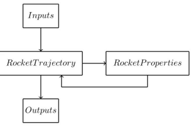
Simulator description

The angle of attack only begins to be calculated in the second phase, as this is when the rocket suffers the first disturbance from the wind. The length of the rod is needed as an input to determine the moment at which the rocket's trajectory becomes unbounded and the angle-of-attack model begins to be calculated.

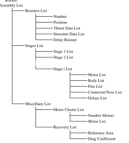
Rocket assembly

Since amplifiers are external components, the structure data list, within the amplifier list (see Figure 5.2), contains additional elements: cylindrical tube lengths and nozzle structures, CP and CNα. The delay of the boosters represents the time between their firing and the moment they are fired, which, at most, should be the moment the first stage body tube is also fired.

Atmospheric model

The last two must provide the respective property for the complete structure of the booster. We can access its data by specifying the name of the model and the required properties.

Wind model

Wind gusts

Since the angle of attack in the simulator only affects thrust, the effect of wind gusts can change the trajectory only if the new solution gives a non-zero angle during the eventual burn. The effect of the wind gust on the angle of incidence 2 s after ignition is shown in Figure 5.14.

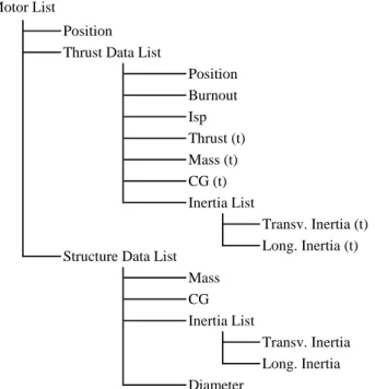
Motors data

Although the main motors' characteristics are found from the thrust profile and other information provided in the data sheets by the methods described in Chapter 4, they are dependent on other data that can only be determined by measurements taken from the motors' dimensions. Therefore, this data must be inserted into the database to automatically calculate the characteristics of the cars.

Drag coefficient model

For all model rocket engines already in the database, their properties are determined based on a final combustion, a deceleration charge (for those that have a deceleration time) and an ejection charge. The thrust profiles are obtained by an interpolated function that fits the points given in the data sheets available online at www.thrustcurve.org.

Validation of the simulator

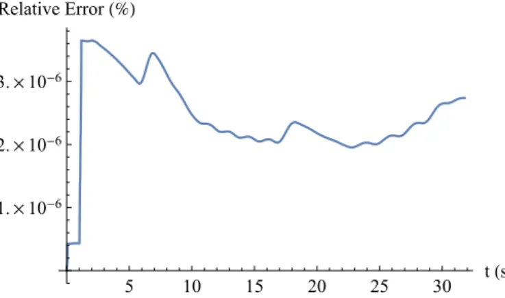
In Figure 5.18 it is represented the rocket's free-fall velocity from the simulator, 10 s after lift-off, under the mentioned conditions. From the values ​​of the relative error, in Figure 5.19, we conclude that the simulator behaves as expected under these conditions.

Rockets description

Model rocket specification

Two types of rockets are used to illustrate the results from the developed simulator: a model rocket and a sounding rocket. The rocket launch model is best suited to observe the effect of wind and ABL on trajectory, as these rockets reach lower velocities and apogees.

Sounding rocket specification

So, from Table 4.1, its drag coefficient is chosen to be 0.695 as it is the midpoint of the respective range. So, again from Table 4.1, we choose a drag coefficient of 0.775, which is the central value of the respective interval.

Rockets characteristics

Model rocket

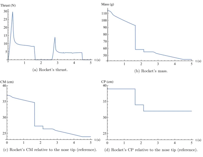
After assembling all the components, the essential data of the sounding rocket is given in Table 6.6. Comparing Figures 6.1c and 6.1d, we conclude that this rocket is always stable since CM, instead of CP, is always closer to the nose.

Sounding rocket

Trajectory simulations conditions

Results from the trajectory simulations

Model rocket launch

Upon reaching apogee, the flight path angle becomes negative as the rocket begins to descend. As the rocket descends, its flight path decreases, meaning its speed steepens.

Sounding rocket launch

Due to the parachute ejection, the rocket suffers a 120g deceleration, which is not shown in Figure 6.8c due to the graphical scale. The flight path angle in Figure 6.8f starts at 90° because the rocket is launched vertically and, again due to the windcock effect, this angle decreases as the rocket follows the direction of the airspeed.

The influence of atmospheric stability

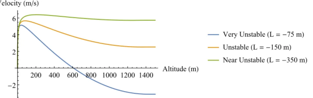
By relating these profiles to the respective trajectories in Figure 6.12, we observe the rocket landing further from the launch site as the atmosphere becomes less unstable, as expected due to the increase in wind speed. The recovery path under a highly unstable atmosphere (see Figure 6.12) stands out because of its different shape.

Simulation rocket and conditions

To study the influence of the exponential rates at which the local weather conditions approximate the data of the developed atmospheric model along the height, these conditions must differ from the defined values ​​in the previous simulations. For the wind speed and direction, their conditions are defined to be the same as those in Table 6.7, respectively.

Landing site uncertainties

Since the rocket follows the direction of the wind speed, the uncertainties of the local wind speed and the surface roughness length (both of which only affect the wind intensity) are expected to change the landing site in this direction, describing a straight line. Partly due to this principle, the uncertainties in wind speed contribute to the lower density of points close to the nearest and furthest distances from the Earth.

Rocket optimization

Likewise, above the ABL, the wind pattern approximates the values ​​given in the CIRA-86 tables. Within the ABL, since wind plays an important role in the trajectory of model rockets, three profiles were proposed and implemented considering the atmospheric stability, which can be inferred from the Obukhov length.

Future work

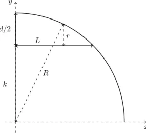
On the extension of the wind profile over homogeneous terrain beyond the surface boundary layer. In Figure B.1, the thick lines represent the half-section of a connector, where Li is the length of the surface, its height, and r1 and r2 are the leading and trailing radius, respectively.