•
,
VOLATILITY MODELLING IN THE FOREX MARKET:
AN EMPIRICAL EVALUATION
J
RENATO G. FLÔRES JR.* and BRUNO B. ROCHE
*EPGE / Fundação Getúlio Vargas, Rio de Janeiro ** École de Commerce Solvay / ULB, Bruxelles
(October, 1999)
We compare three frequently used volatility modelling techniques: GARCH, Markovian switching and cumulative daily volatility models. Our primary goal is to highlight a practical and systematic way to measure the relative effectiveness of these techniques. Evaluation comprises the analysis of the validity of the statistical requirements of the various models and their performance in simple options hedging strategies. The latter puts them to test in a "real life" application. Though there was not much difference between the three techniques, a tendency in favour of the cumulative daily volatility estimates, based on tick data, seems dear. As the improvement is not very big, the message for the practitioner - out of the restricted evidence of our experiment - is that he will probably not be losing much if working with the Markovian switching method. This highlights that, in terms of volatility estimation, no dear winner exists among the more sophisticated techniques.
イ⦅セZMZZMZセiZco[M[tセeZcc[GェaNcN}@
.. • I a L CUí clMONSENO Hl'NR - S
MARI : . li L' VG., fU.i- • ÇAO G .
1. INTRODUCTION
This paper presents an empirical comparison of frequently used volatility modelling techniques. Our primary goal is to highlight a practical and systematic way to measure the relative effectiveness of these techniques. We evaluate the quality of GARCH, Markovian switching and cumulative daily volatility (cdVol) models, based on daily and intra-day data, in forecasting the daily volatility of an exchange rate data series. The analysis considers both the models' residuais and the performance of simple options hedging strategies. The former deals with the validity of the statistical requirements of the various models, while the latter puts them to test in a (close to) "real lífe" application. The residuais' analysis deals with the distributional properties of the standardised returns - using the continuously updated volatilities - which are usually assumed to be normal. This provides a uniform frarnework to compare models which have a more complete statistical structure with others, less complete, where a residual terrn, in the classical sense, does not exist. While GARCH and Markovian switching structures belong to the first class, cdVol computations should be included in the second.
Though we have not found much difference between the techniques tested, GARCH estimates perforrned poorly in the options hedging and a tendency in favour of the cumulative daily volatility estimates, based on tick data, seems clear. Given that cdVol procedures use much more information than the other altematives, this might have been expected.
As the improvement is not very big, and periods of market inefficiency were detected, the message for the practitioner - out of the restricted evidence of our experiment -, is that, if either access to or manipulation of tick data is difficult, he might not be losing mueh if working with the other two methods. Notwithstanding, as a second best, results slightly favour the Markovian switching method.
The lack of a conclusive winner draws attention to the need of more studies of this kind. lndeed, we stiU are at crossroads in terms of volatility estimation, no clear optimum existing arnong the more sophisticated teehniques.
upon the two evaluation strategies, while section 5 presents the empirical results. The final section conc1udes.
2. DATA DESCRIPTION
We use daily observations (recorded at 10pm GMT) of the Deutsche Mark (DEM) against the US dolIar (USD), from October 1995 to October 1998 (784 trading days in total). We also use interbank tick-by-tick quotes of foreign exchange (forex) rates, supplied by Reuters via Olsen & Associates, and over-the-counter currency options data, interbank, lOpm, lmonth, at-the-money implied volatility.
2.1. Intraday data and the foreign exchange interbank market
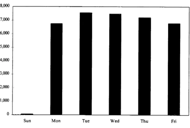
The interbank market, in contrast with other exchange markets, has no geographical limitations (currencies are traded alI over the world) and no trading-hours scheme (currencies are traded alI around-the-c1ock): it is truly a 24hours, 7days-a-week market. Naturally, there are significant intraday, intraweek and intrayear seasonal pattems (see Figures 1 and 2), explained respectively by the time zone effect (in the case of the USDIDEM rate, the European and the US time zones are the most active ones), the low activity exhibited during weekends and some universal bank holidays (eg: Christmas, New Year). Some other factors such as the release of economic indicators by central banks may also have an effect on the structural seasonality observed in foreign exchange markets.
Forex traders negotiate deals and agree transactions over the telephone, trading prices and volumes being not known to third parties. The data we use in this study are the quotes from a large data supplier (Reuters). These quotes are provided by market-makers and conveyed to data subscribers terminals. They are meant to be indicative, providing a general indication of where an exchange rate stands at a given time. Though not necessarily representing the actual rate at which transactions really took place, these indicative quotes are felt as being fairly accurate and matching the true prices experienced in the market.1 Moreover, in order to avoid dealing with the bid-ask issue,
inherent to most high frequency data (see, for instance, Chapter 3 in CampbelI et aI.
J The professionalism ofthe market-makers (whose credibility and reputation depend on their relationship
(1997)), use was made in this study ofthe bid series only, generally regarded as a more consistent set of observations.
Further description of questions related to intra-day data in forex markets can be found in Baillie and Bollerslev (1989), Goodhart and Figliuoli (1991), Müller et aI. (1997) and Schnidrig and Würtz (1995), among others.
2.2. Exchange rate retums
Traditionally, retums on forex series are continuously compounded returns. They are ca1culated as the difference in natural logarithm of the exchange rate value SI for two consecutive observations : rI
=
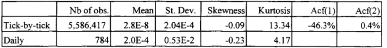
100[ln(SI) - In(SI-l)].Table 1 shows the basic descriptive statistics for the USDIDEM foreign exchange retums, for the ticks and daily data. There is an enormous difference between the first two moments of the series, confmning the dramatic effect of time aggregation, Ghysels et al. (1998). Daily data are quite spread out, with a coefficient of variation (CV) of 26.65, but tick data are considerably more, with a CV 274 times higher. Moreover, their kurtosis is also much higher.
The ticks series allow the examination of intra-day, intra-week and intra-year (or inter-month) pattems, Guillaume et al. (1997). Figures 1 and 2 show, respectively, the intra-day and intra-week pattems.
Table 1. Descriptive statistics ofthe daily and tick-by-tick retums.
Nb ofobs. Mean St. Dev. Skewness Kurtosis Acf(l) Tick-by-tick 5,586,417 2.8E-8 2.04E-4 -0.09 13.34 -46.3%
Daily 784 2.0E-4 0.53E-2 -0.23 4.17
2.3. Implied volatility - the Black-Scholes model
The language and conventions of currency option trading are drawn from the Black-Scholes-Merton model, Black and Scholes (1973), even though neither traders nor academics believe in its literal truth. The model assumes that the spot exchange rate follows a geometric Brownian motion, in which the constant term of the drift equals r-r* , the difference between the risk-free, continuously compounded domestic and
- - - -
_ .-foreign interest rates. The drift and the constant volatility parameter cr are supposed
known.
Logarithrnic exchange rate returns are then normally distributed, and formulas for European put and call values can be obtained. That for a call is
(1)
where St represents the spot forex rate at time t, 't the time to maturity, X the strike price and <1>(.) is the standard cumulative normal distribution function.
Market participants use these formulas even though they do not consider the Black-Scholes model a precise description of how exchange rates actually behave. We shall follow this practice and, for the second evaluation strategy, carry out numerical procedures using formula (l) without necessarily agreeing with the mode!.
There is a one-to-one relationship between the volatility parameter cr and the Black-Scholes pricing function, for fixed values of the remaining arguments. This allows market prices of calls and puts to be expressed in units of volatility, called the Black-Scholes implied (ar implicit) volatility. Traders quote options in terms of implied volatility. Prices are determined by the market; the Black-Scholes pricing function simply transforms them from one metric to another, when dealers invert function (1) to calculate an implied volatility. The value obtained becomes an estimate of the risk-neutral standard deviation of logarithrnic changes in the forward exchange rate.
exerci se price, and translate the agreed price from vols to marks per dollar of notional
undedying value, by substituting the current spot rate, one-month domestic and foreign interest rates, the contractually-agreed maturity (here, one month), exercise price and vol into the Black-Scholes formula (1).
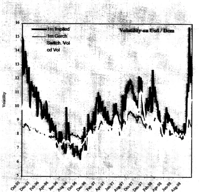
Figure 3 shows the graph of the implied (one-month) at-the-money volatility computed for the daily series.
3. A BRIEF REVIEW OF THE METHODS
Since important and encompassing empirical studies like Hsieh's (1988), forex retums have been recognised to exhibit heteroskedasticity and leptokurticity. Yet, there is no agreement regarding the best process to describe their series. Different models capture, with more or less success, these features. In this paper we work with three of them: the GARCH c1ass of models initiated by Bollerslev (1986), the Markovian Switching Models as proposed by Hamilton (1989, 1990) and the Cumulative Daily Volatility (cdVol) models based on tick data developed by Zhou (1996 a, b). The first two are fulI statistical models, suitable to daily observations. The last one is a procedure which, from intraday data, produces an estimate of daily volatilities.
3.1. The GARCH models
The GARCH class has become very popular in finance for modelling time varying volatility in forex markets, Bollerslev et alo (1992), Bollerslev et aI. (1993). It provides a parsimonious representation which portrays well the volatility cluster effect; however, it
builds up a deterministic rather than a stochastic function of past information and does not account for the possibility that either some latent factors or the distribution generating the returns change. Indeed, it is this rather inertial characteristic of its models that is responsible for their most inconvenient properties.2
Perhaps the most widely used member of this large family is the GARCH( 1,1 ) model which has the form:
Etl It-1 - N(O,I) and
2 For a further criticism on the ARCH/GARCH family see, for instance, Bera and Higgins (1995), and
2 2 A 2
a t
=
ú) + a Y t-I+ I-' a t-I (2)where rt is the naturallogarithrn rate of return;
e
is the expected return conditional onIt-I, the market information available at time t-l ; a2t is the variance at time t of the
prediction erro r conditional on It-I ,and ú), a,
p
are real coefficients, assumed nonnegative.
For stability of the volatility process, the sum of a and
p
must be less than one.Moreover, from (2), it is immediate to see that:
(3)
Figure 1. Intra-day pattem USD IDEM (Average number oftransactions per hour)
セNMMMMMMMMMMMMMMMMMMMMMMMMMMMMMMMMMMMMMMMMMMMMMMMMMMMセ@
800
--700
600
-500
400
-300
200
-o
I 2 3 4 5 6 7 8 9 10 11 12 13 14 15 16 17 18 19 20 21 22 23Hour (GMn
3.2. The Markovian Switching mo deis
The volatility switching models, inspired in earlier work by Goldfeld and Quandt (1973) and successfully tested by Rockinger (1994) on stocks, deseribe returns as being
---.---distributions is detennined in a Markovian manner. Volatility becomes then a stochastic function of past infonnation. Though the number of regimes is arbitrary, the model becomes cumbersome and sometimes difficult to work with when allowing for more than three states.
Figure 2. Intra-week panem USDIDEM (Average number oftransactions per day-of-the-week)
8,000 , - - - -_ _ _ _ _ _ _ _ _ _ _ _ _ _ _ _ _ _ _ ---,
7,000
6,000
5,000
4,000
3,000
2,000
1,000
O.l...-_ ... _ _ _
Sun Mon Tue Wed Thu Fri
Retums are accordingly modelled as switching processes whose shocks are independent from the states. The shocks are usually drawn from a nonnal N(O,l) distribution. Assuming, as in this paper, that the variance can switch between only two different regimes, we can write the following equations:
(4)
where croand cri represent the values ofthe two unconditional volatility regimes, {Cd is a Markov chain with values in {O,l} and transition probabilities { poo. PIO. POI. PI
d
such that :and PIO+poo=1 (5)
3.3. The Cumulative Daily Volatility model (cdVol)
The third technique has been made possible thanks to the increasing power of computers, which has allowed the development of means of storing and dealing with high frequency financiaI data. These new information technologies opened the possibility to study volatility in greater detail, Dunis (1989), Pictet et aI. (1992).
In high frequencies, heteroskedasticity usually increases with the sampling frequency, due to the fact that the variance ofthe noise inherent to the recording process becomes comparable (even greater than) to the one among the different observed retums, Zhou (1 996b ). A way to deal with this is to anaIyse observations at unequally spaced time periods. The procedure of de-volatilisation developed by Zhou (1995) suggests taking more observations in volatile periods and less in quieter ones. This process of obtaining time series with constant volatility re-scaIes time in a adaptive fashion; the picking frequency or, the time interval between two observations, adjusts to the instantaneous volatility observed tick-by-tick.
Another way to deal with heteroskedasticity, in equally spaced time series as in this paper, is to normalise the returns by their daily cumulative volatility (cdVol). In this case, each daily cumulative volatility is computed from tick-by-tick intraday data within a 24-hour period.
The de-volatilisation and normalisation algorithm developed by Zhou (1996 a, b) is based on a volatility estimator which, from high-frequency tick data, computes the cumulative daily volatility for a set period, say a day or a week. The formula for daily volatility is (Zhou (1996 a»:
(6)
4. THE EVALUATION STRATEGY
In the first two models previously discussed, the residuaIs should be normal and non-correlated, in the last one, standardised returns should follow a normal distribution. However, as can be seen from (3) and (4), conveniently standardised returns in the first two models should also be iid N(O,I). The same could be expected if returns are standardised by the implicit volatility. This fact provides a common ground for statistically comparing all models at stake, and our first evaluating criterion consists in a thorough residuaIs, i.e. standardised returns, analysis, testing alI normality assumptions. For the latter, to make things easily reproducible, we have used the two common Jarque-Bera, Jarque and Bera (1980), and Kolmogorov-Smimov tests.
Evaluation also comprises checking the volatility models through their performance in a volatility hedging strategy. As known in these cases, Gavridis and Dunis (1998), if the volatility estimate is higher than the implied volatility (plus a volatility threshold of say 1%) one should go long on the volatility, going short otherwise. If the difference between the "filtered" volatility estimate and the implied volatility is, in absolute value, no greater than the given volatility threshold (here 1 %) , stay neutral. In this example, the position should be kept until the option expires. The figure of merit in this evaluation strategy is the amount of money made or loss (in our case, the amount of Deutsche Marks) at the option's expiry date. In other words, the result is the difference between the strike price and the spot price at the option's expiry. In order to have a background comparison, a random strategy and systematic - long and short - strategies were also used.
5. THE EMPIRICAL RESUL TS
5.1. Basic statistics.
Table 2 shows the results of the GARCH(1,I) estimation, obtained through maximum likelihood (ML) under the normality assumption for the residuais. The key coefficients (a and
P)
are significant at 1 %, though there is strong evidence that the process is integrated (a+p=0.988).regimes. All coefficients are significant at 5%. The probability of staying in the higher volatility regime (Ct =0) is 0.8049, what means that, on average, it lasts for about five
days ( 1/(1-0.8049) = 5.13 ; see also Hamilton (1989)).
For computing the cdVol, the values were obtained on a daily basis. Day t begins at 10:00 pm and ends 24 hours later (the first day is October 1 st, 1995). Intraday observations during day t are denoted by ti , i=0,1,2, .... At the beginning ofthe day, the first intraday observation has value S(lo), and the corresponding initial value of the cumulative daily volatility, cdVol(O), is zero. Assume now that, in the current day t, the most recent element ofthe tick series is obtained at time ti : S(ti). One then estimates: - the volatility increment V(ti-l,ti) using formula (6) described in section 3, and setting, as in Zhou (1998), the parameter k for the optimal standard error (in this study, k=7);
the updated cumulative volatility within the 24-hour period (ie: until ti does not exceed 10:00 pm ofthe following trading day) as follows:
cdVol(i) = cdVol(i-l) + V(ti-l, ti)
Table 2. GARCH(I,I): Empirical Results.
Value Std. Error t Value Pr(>t)
e
0.02E-2 0.00019 1.0 0.16CJ) 3.42E-7 0.00000 1.8 0.04
a 0.019 0.00748 2.5 0.01
f3
0.969 0.01287 75.3 0.00Table 3. Markov switching model- results.
Value Std. Error t Value Pr(>t)
e
0.0345 0.0171 2.023 0.02150'0 0.6351 0.0281 22.603 0.0000
O'J 0.2486 0.0313 7.934 0.0000
poo 0.8049 0.0620 12.976 0.0000
Pll 0.6348 0.0927 6.848 0.0000
The cdVol(i) value obtained for the last observation of day t wiIl be the cumulative daily volatility estimate (ofthe day).
Figure 3 is a graphical summary of the volatilities estimated by the three methods, together with the implicit volatility series computed as described in section 2. During most of the period under study the implied volatility is superior to the three other estimates.
Figure 3. Volatility estimates, various techniques .
5.2. Residuais Analysis
We now carry out a brief analysis of the residuals computed from the four models: the implied volatility model, the GARCH model, the Markovian switching model with two volatility regimes and the cumulative daily volatility model (cdVol). Strictly speaking, the term residuaIs - as explained in the previous section - is here used for the series of standardised returns. Standardisation uses the forecasted volatilities and -according to the case - other parameters in the model as well. If the volatility captures well the fluctuations of the market, and the models' assumptions are valid, such "residuals" are expected to be normal.
Table 4 presents the basic summary statistics and normality tests for the standardised log-returns and the standardised residuals/returns computed from the four procedures. Figures 4 to 6 show the probability plots of the standardised returns from the GARCH(l,l), the Switching and the cdVol models.
Table 4. Residuals from the tive models - basic statistics and normality tests.
raw log retums
implied garch(l,I)
volatility Im volatility
markovian switching
cum. daily. volatility
Mean 0.0043 0.0425 0.0454 0.0485 0.0879
Std. Dev. 0.9944 0.9218 0.9708 1.0804 0.9525
Skewness -0.2455 -0.3257 -0.2191 -0.1344 0.1031
exc. Kurtosis 1.2764 2.0871 0.8518 1.2228 -0.1167
Sample Size 783
Ljung-Box(20 lags) criticaI value at 5% = 31.4
- raw std residuais 25.33 22.4 23.5 23.6 21.5
- squared std residuais 43.82 12.2 13.8 16.9 14.8
Normality Tests
Jarque & Bera 58.68 149.99 28.79 49.18 1.76
**
**
**
**
Kolmogorov Smimov 0.0607 0.0553 0.0502 0.0570 0.0226
p. value 0.0000 0.0000 0.0001 0.0000 0.5000
***
denotes parameter estimates statistically significant at the one percent leveiThe striking feature is that alI models capture fair1y well the heteroskedasticity of the under1ying time series ( as shown by the Ljung-Box test on the squared residuals )
Figure 4. ProbabiIity pIot ofthe GARCH(l,l) model.
N
"'!" o o
-3 -2 -1 o 2
Quantiles of Standard Normal
Figure 5. Probability pIot of the Markov switching model.
.... 1
NJ
..
I
ãi
" I
"C
0)
"iõ
"
Ir
r.
セ@
I
セ@
Cf)
')I
ocP o ..,. o
o
-3 -2 -1 o 2 3
Quantiles of Standard Normal
o
o
Figure 6. Probability plot of the cdVol Model residuais
M o
N
セセ@
I o o olMMLMMMMMLMMMMMMLMMMMMLMMMMMMLMMMMMMイMMMMMNMセ@
-3 -2 -1 o 2 3
Quantiles of Standard Normal
5.3. Volatility estimates analysis via Volatility Hedging Strategies
As previously said, if the filtered volatility estimate is greater than the implicit volatility (plus the volatility threshold), one goes long in the volatility; if the filtered volatility estimate is smaller than the implicit volatility (minus the volatility threshold). one goes short; staying neutral otherwise; and keeping the position until the option expires.
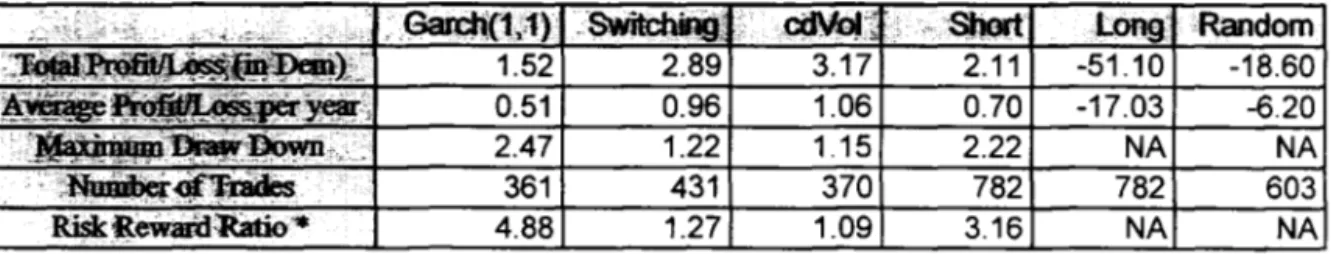
We here compare hedging strategies using the GARCH(l,I), the Markov Switching and the cdVol estimated volatilities. In order to have a set of background vaIues, a random strategy, a systematic short strategy (ie: go short every day) and a systematic long strategy (ie: go long every day) were used.
Table 5. Summary results of options strategies.
」ゥZャyーエセ@ .. • ... $)art' long oRandom 3.17 2.11 -51.10 -18.60 1.06 0.70 -17.03 -6.20
1.15 2.22 NA NA
370 782 782 603
RiskRewarol&tio.. 4.88 1.27 1.09 3.16 NA NA
*
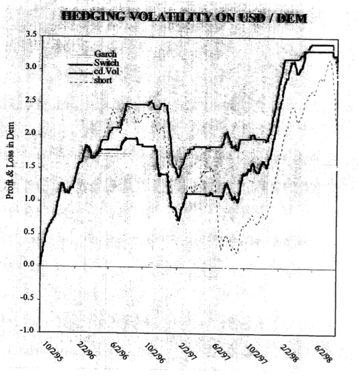
Here defmed as the ratio Maximum Drawdown / A verage Profit per Year.Figure 7 displays the daily profit & loss trajectories for the four hedging strategies which showed positive profits. During most of the time span the cdVol curve dominates the other three. The figure also suggests a somewhat poor performance for the GARCH strategy.
6. CONCLUSIONS
We studied the behaviour ofthree popular volatility models in a USDIDEM daily forex series. In terms of residuais analysis, the cdVol model best captured the normality structure of returns, according to the two goodness-of-fit tests used. GARCH and Markovian residuais presented a somewhat high excessive kurtosis and failed to pass them.
When compared within a hedging framework, all strategies showed positive results and outperformed a random strategy, though the cdVol and the Switching Volatility strategies performed slightly better, with the GARCH hedge failing to beat a short strategy. The fact that a constant short volatility strategy generated profits denotes periods of market inefficiencies.
As a further extension, an economic interpretation of these results should be
considered. The existence of long-lasting periods of inefficiencies in a very liquid derivative market and the similar behaviour of the volatility modelling techniques, during periods of the hedging experiment - even though, in almost ali terms, the cdVol model was superior - are issues that deserve more attention.
Figure 7. Graphical Results (daily profit & loss curve).
0.0 +----,--'----.---r.:.=... ':"'--r---.,-,-'-, _
-0.5
.' , ,
, ;
1\ ,
\ ,
,
"
I
,
, : , '
/'1
Finally, this comparison framework should be tried in other, non-continuous trading markets, as those for stocks and interest rates. This would shed more light on the points raised here and help in choosing among the three techniques considered.
REFERENCES
Baillie R. and T. Bollerslev (1989), 'Intra-day and inter-market volatility in exchange rates' Review of Economic Studies 58, 565-585.
Bera, A K. and M. L. Higgins (1995), 'On ARCH Models: Properties, Estimation and Testing', in L. Exley, D. A. R. George, C. J. Roberts and S. Sawyer [eds.], Surveys in Econometrics, Basil Blackwell, Oxford.
Black F. and M. Scholes (1973), 'The pricing of Options and Corporate Liabilities', Journal of Polítical Economy 81, 637-59.
Bollerslev T. (1986), 'Generalized Autoregressive Conditional Heteroskedasticity', Journal ofEconometrics 31,307-327.
Bollerslev T., R. Chou, K. Kroner (1992), 'ARCH Modeling in Finance: A Review of the Theory and Empirical Evidence', Journal of Econometrics, 52, 5-59.
BOllerslev T., R. Engle, D. Nelson (1993) 'ARCH Models', in R. F. Engle and D.McFadden [eds.], Handbook of Econometrics, VoI. 4, North Holland, Amsterdam. Campbell J. Y., A. W. Lo and A. C. MacKinlay (1997), 'The Econometrics of Financiai
Markets', Princeton University Press, Princeton, New Jersey.
Dunis C. (1989), 'Computerised Technical Systems and Exchange Rate Movements', chapter 5, 165-205, in C. Dunis and M. Feeny [eds.], Exchange Rate Forecasting, Probus Publishing Company, Cambridge, UK.
Flôres, R. G., Jr. (1996), 'Crises and Volatility', Proceedings of the 3rd Conference on Forecasting Financiai Markets, Imperial College and Chemical Bank, London.
Fernandes, M. (1999), 'Essays on the Econometrics ofContinuous-time Finance', These
presentée en vue de I' obtention du grade de Docteur en Sciences de Gestion, École de Commerce Solvay, Université Libre de Bruxelles, Bruxelles.
Gavridis, M. and C. Dunis (1998), 'Volatility Trading Models : an application to daily exchange rates" Derivative Use, Trading and Regulation Nl, p9-16
Ghysels, E., C. Gouriéroux and J. Jasiak (1998) 'High frequency financiaI time series data: some stylized facts and mo deIs of stochastic volatility', Chapter III.7 in C. Dunis and B. Zhou [ed], Nonlinear Modelling of High Frequency Financiai Time Series, , John Wiley & Sons, Chichester.
Goldfeld S. and R. Quandt (1973), 'A Markov model for switching regressions', Journal of Econometrics 1, 3-16
Goodhart C. and L. Figliuoli (1991), 'Every minute counts In financiaI markets' Journal of International Money and Finance 10, 23-52
GuiUaume D., M. Dacorogna, R. Davé, U. Müller, R. Olsen and O. Pictet (1997),'Frorn the bird's eye to the microscope: a survey ofnew stylized facts ofthe intra-daily foreign exchange markets', Finance and Stochastics 1,95-129.
Hamilton J. (1989), 'A new approach to the economic analysis of nonstationay time series and the business cycle', Econometrica 57, 357-84.
Hamilton J. (1990), 'Analysis of time series subject to change in regine' Journal of Econometrics 45, 39-70.
Hamilton J. and R. Susmel (1994), 'Autoregressive Conditional Heteroskedasticity and Changes in Regime', Journal of Econometrics 64, 307-333.
Hsieh D. (1988), 'The statistical properties of daily foreign exchange rates: 1974-1983' Journal of International Economics 24, 129-145
Hsieh D. (1989), 'Modeling heteroskedasticity in daily foreign exchange rates' Journal of Business and Economic Statistics 7, 307-317.
Jarque C. M. and A. K. Dera (1980) 'Efficient tests for normality, homoscedasticity, and serial independence regression residuaIs' Economic Letters 6, 225-259.
Kai J. (1994) 'A Markov Model of Switching-Regime ARCH', Journal of Business &
Economic Statistics, 12, 3, 309-316.
Müller U., M. Dacorogna, D. Davé, R. Olsen, O. Pictet and J. Von Weizsãcker (1997), 'Volatilities of Different Time Resolutions - Analyzing the Dynamics of Market Components', Journal of Empirical Finance 4, no. 2-3,213-240.
Pictet O., U. Müller, R. Olsen and J. Ward (1992), "Real-Time Trading Models for Foreign Exchange Rates", The Journal of Neural and Mass-Parallel Computing and Information Systems, Neural Network World 2, no. 6, 713-725.
Rockinger M. (1994) 'Regime switching: evidence for the French stock market', Working paper, HEC School ofManagement, Paris
Schnidrig R. and D. Würtz (1995), 'Investigation of the volatility and autocorrelation function ofthe USDIDEM exchange rate on operational time scales', Paper presented at the 'High Frequency Data in Finance' Conference (HFDF-I), Zürich.
Zhou B. (1995), 'High Frequency Data and Volatility in Foreign Exchange Rate', Working paper 3739, MIT Sloan Schoold ofManagement, Mass.
Zhou B. (1996a), 'Forecasting foreign exchange rates subject to devolatilization', chapter 3, 51-67, in C. Dunis [ed.], Forecasting Financiai Markets, John Wiley & Sons, Chichester.
Zhou B. (1996b), 'High Frequency Data and Volatility in Foreign Exchange Rates', Journal ofBusiness and Economics Statistics, 14,45-52.
ENSAIOS ECONÔMICOS DA EPGE
336.
TIME-SERIES PROPERTIES ANO EMPIRICAL EVIDENCE OF GROWTH ANO INFRASTRUCTURE (REVISED VERSION) - João Victor Issler e Pedro Cavalcanti Ferreira - Setembro1998 - 38
pág.337.
ECONOMIC LIFE OF EQUlPMENTS ANO DEPRECIATION POLICIES - Clovis de Faro - Outubro1998 - 18
pág.338.
RENDA PERMANENTE E POUPANÇA PRECAUCIONAL: EVIDÊNCIAS EMPÍRICAS PARA0 BRASIL NO PASSADO RECENTE (VERSÃO REVISADA) Eustáquio Reis, João Victor Issler, Fernando Blanco e Leonardo de Carvalho-Outubro
1998 - 48
pág.339.
PUBLIC VERSUS PRIVATE PROVISION OF INFRASTRUCTURE - Pedro Cavalcanti Ferreira - Novembro1998 - 27
pág.340.
"CAPITAL STRUCTURE CHOICE OF FOREIGN SUBSIDIARIES: EVIDENCE FORM MULTINATIONALS IN BRAZIL" Walter Novaes e Sergio R.C.Werlang -Dezembro1998 - 36
pág.341.
THE POLITICAL ECONOMY OF EXCHANGE RATE POLICY IN BRAZIL:1964-1997 -
Marco Bonomo e Cristina Terra - Janeiro1999 - 46
pág.342. PROJETOS COM MAIS DE DUAS VARIAÇÕES DE SINAL E O
CRITÉRIO DA T
AX.AINTERNA DE RETORNO - Clovis de Faro e Paula de
Faro - Fevereiro 1999 - 31 pág.
343. TRADE BARRIERS AND PRODUCTIVITY GROWTH:
CROSSINDUSTRY EVIDENCE Pedro Cavalcanti Ferreira e José Luis Rossi
-Março 1999 - 26 pág.
344. ARBITRAGE
PRICING
THEORY
(APT)
E
VARIÁVEIS
MACROECONÔMICAS - Um Estudo Empírico sobre o Mercado Acionário
Brasileiro - Adriana Schor, Marco Antonio Bonomo e Pedro L. VaUs
Pereira-Abril de 1999 - 21 pág.
345. UM MODELO DE ACUMULAÇÃO DE CAPITAL FÍSICO E HUMANO:
UM DIÁLOGO COM A ECONOMIA DO TRABALHO - Samuel de Abreu
Pessôa - Versão Preliminar: Abril de 1999 - 24 pág.
346. INVESTIMENTOS, FONTES DE FINANCIAMENTO E EVOLUÇÃO DO
SETOR DE INFRA-ESTRUTURA NO BRASIL:
1950-1996 - Pedro
Cavalcanti Ferreira e Thomas Georges Malliagros - Maio de 1999 - 42 pág.
348. ENDOGENOUS TIME-DEPENDENT RULES AND INFLATION INERTIA - (Preliminary Version) - Marco Antonio Bonomo e Carlos Viana de Carvalho - Junho de 1999 - 22 pág.
349. OPTIMAL STATE-DEPENDENT RULES, CREDffiILITY, ANO
INFLATION INERTIA - Heitor Almeida e Marco Antonio Bonomb - Junho de 1999 - 34 pág.
350. TESTS OF CONDITIONAL ASSET PRICING MODELS IN THE BRAZILIAN STOCK MARKET - Marco Bonomo e René Garcia - Julho de 1999 - 35 pág.
351. INTRODUÇÃO
À
INTEGRAÇÃO ESTOCÁSTICA (Revisado em Julho de1999) - Paulo Klinger Monteiro - Agosto de 1999 - 65 pág.
352. THE IMPORTANCE OF COMMON-CYCLICAL FEATURES IN VAR ANAL YSIS: A MONTE-CARLO STUDY (Preliminary Version) - Farshid Vahid e João Victor Issler - Setembro 1999 - 41 pág.
353. ON THE GROWTH EFFECTS OF BARRIERS TO TRADE - Pedro Cavancanti Ferreira e Alberto Trejos - Setembro 1999 - 31 pág.
354. FINANCE AND CHANGING TRADE PA TTERNS IN BRAZIL - Cristina T. Terra - Setembro 1999 - 45 pág.
355. ECONOMIA REGIONAL, CRESCIMENTO ECONÔMICO E
DESIGUALDADE REGIONAL DE RENDA Samuel de Abreu Pessôa -Setembro de 1999 - 9 pág.
356. ECONOMIA REGIONAL E O MERCADO DE TRABALHO - Afonso Arinos de Mello Franco Neto - Setembro de 1999 - 26 pág.
357. "WE SOLD A MILLION UNITS" - THE ROLE OF ADVERTISING PAST-SALES - Paulo Klinger Monteiro e José Luis Moraga-González - Outubro de
1999 - 28 pág.
358. OPTIMAL AUCTIONS IN A GENERAL MODEL OF IDENTICAL GOODS - Paulo Klinger Monteiro - Outubro de 1999 - 17 pág.
359. DISCRETE PUBLIC GOODS WITH INCOMPLETE INFORMATION -Flavio M. Menezes, Paulo Klinger Monteiro e Akram Temimi - Outubro de 1999 - 33 pág.
360. SYNERGIES AND PRICE TRENDS IN SEQUENTIAL AUCTIONS - Flavio M. Menezes e Paulo Klinger Monteiro - Outubro de 1999 - 19 pág.
361. VOLA TILITY MODELLING IN THE FOREX MARKET: AN EMPIRICAL EVALUATION - Renato G. Flôres Jr. e Bruno B. Roche - Novembro de 1999 -23 pág.
I
/
... f .... •
000090827
FUNDAÇÃO GETULIO VARGAS
BIBUOTECA
ESTE VOLUME DEVE SER DEVOLVIDO À BIBLIOTECA NA ÚL liMA DATA MARCADA
N.Cbam. PIEPGE EE 361
Autor: FLÔRES JUNIOR, Renato Galvão
Título: Volatility modelling in the forex market : ao empiri
1111111111111
セセXRW@
FGV -BMHS N"