Forecasting daily volatility using high frequency financial data

(1)

FUNDAÇÃO GETULIO VARGAS

SÃO PAULO SCHOOL OF ECONOMICS

THIAGO WINKLER ALVES

FORECASTING DAILY VOLATILITY USING HIGH

FREQUENCY FINANCIAL DATA

SÃO PAULO

(2)

THIAGO WINKLER ALVES

FORECASTING DAILY VOLATILITY USING HIGH

FREQUENCY FINANCIAL DATA

Dissertation presented to the Professional Master Program from the São Paulo School of Economics, part of Fundação Getulio Vargas, in partial fulﬁllment of the requirements for the degree of Master of Economics, with a major in Quantitative Finance.

Supervisor:

Prof. Dr. Juan Carlos Ruilova Terán

(3)

Winkler Alves, Thiago.

Forecasting Daily Volatility Using High Frequency Financial Data / Thiago Winkler Alves – 2014.

77f.

Orientador: Prof. Dr. Juan Carlos Ruilova Terán.

Dissertação (MPFE) – Escola de Economia de São Paulo.

1. Mercado financeiro - Modelos econométricos. 2. Análise de séries temporais. 3. Mercado futuro. I. Ruilova Terán, Juan Carlos. II. Dissertação (MPFE) – Escola de Economia de São Paulo. III. Título.

(4)

THIAGO WINKLER ALVES

FORECASTING DAILY VOLATILITY USING HIGH

FREQUENCY FINANCIAL DATA

Dissertation presented to the Professional Master Program from the São Paulo School of Economics, part of Fundação Getulio Vargas, in partial fulﬁllment of the requirements for the degree of Master of Economics, with a major in Quantitative Finance.

Date of Approval: August 6th_{, 2014}

Examining Committee:

Prof. Dr. Juan Carlos Ruilova Terán

(Supervisor) Fundação Getulio Vargas

Prof. Dr. Alessandro Martim Marques

Fundação Getulio Vargas

Prof. Dr. Hellinton Hatsuo Takada

(5)

(6)

ACKNOWLEDGEMENTS

To my grandmothers and parents, who taught me and my sister how important studying is. She, even six years younger, keeps inspiring me with her daily conquests.

To Vicki, because revising the English in my writing was the smallest contribution she ever made me. Thank you for all the support, even when it meant I would be away.

To all my Professors, but especially to Prof. Dr. Juan Carlos Ruilova Terán and Prof. Dr. Alessandro Martim Marques, for all the knowledge and precious advice given.

To all my friends and colleagues, particularly to Wilson Freitas and Thársis Souza, who are always available to sit at a bar table and talk ﬁnance while drinking beer.

(7)

(8)

ABSTRACT

Aiming at empirical findings, this work focuses on applying the HEAVY model for daily volatility with financial data from the Brazilian market. Quite similar to GARCH, this model seeks to harness high frequency data in order to achieve its objectives. Four variations of it were then implemented and their fit compared to GARCH equivalents, using metrics present in the literature. Results suggest that, in such a market, HEAVY does seem to specify daily volatility better, but not necessarily produces better predictions for it, what is, normally, the ultimate goal.

The dataset used in this work consists of intraday trades of U.S. Dollar and Ibovespa future contracts from BM&FBovespa.

(9)

RESUMO

Objetivando resultados empíricos, este trabalho tem foco na aplicação do modelo HEAVY para volatilidade diária com dados financeiros do mercado Brasileiro. Muito similar ao GARCH, este modelo busca explorar dados em alta frequência para atingir seus objetivos. Quatro variações dele foram então implementadas e seus ajustes comparadados a equivalentes GARCH, utilizando métricas presentes na literatura. Os resultados sugerem que, neste mercado, o HEAVY realmente parece especificar melhor a volatilidade diária, mas não necessariamente produz melhores previsões, o que, normalmente, é o objetivo final.

A base de dados utilizada neste trabalho consite de negociações intradiárias de contratos futuros de dólares americanos e Ibovespa da BM&FBovespa.

(10)

List of Figures

Figure 1 – Weak-sense stationarity example . . . 20

Figure 2 – Random walk example . . . 22

(11)

List of Tables

Table 1 – Time series of AAPL prices . . . 18

Table 2 – Description of the dataset . . . 47

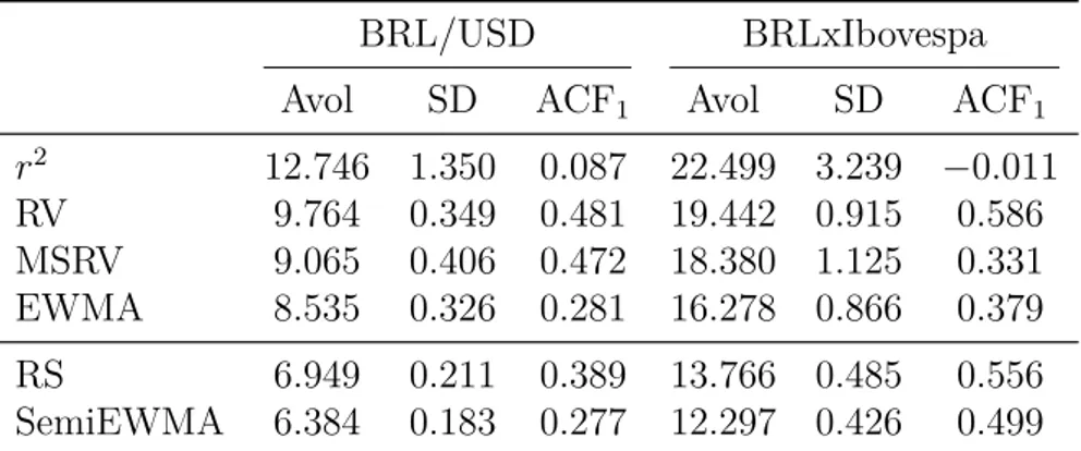
Table 3 – Summary statistics for the dataset . . . 48

Table 4 – χ2_{(1) signiﬁcance levels} _{. . . 49}

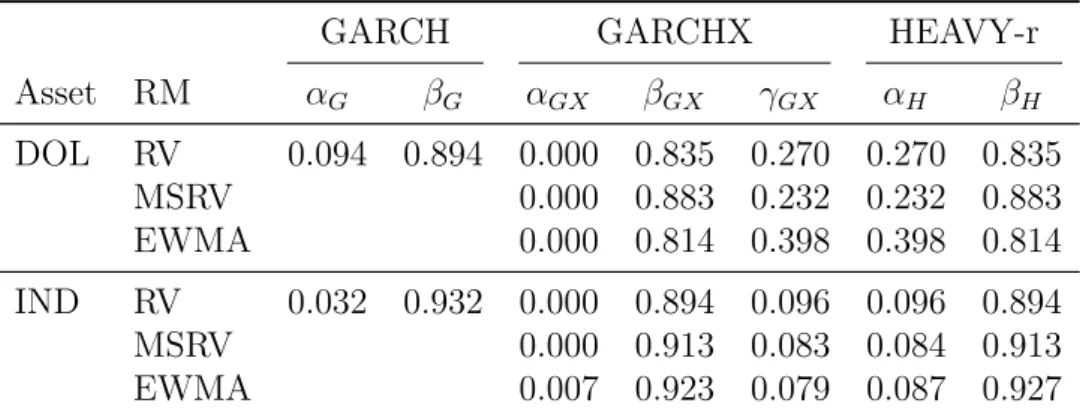
Table 5 – Parameters comparison: GARCH x GARCHX x HEAVY-r. . . 52

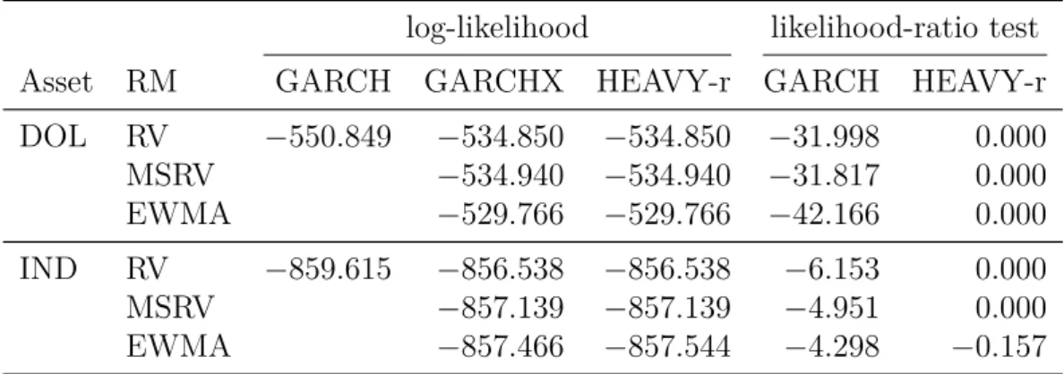
Table 6 – Models’ log-likelihood and likelihood-ratio test versus GARCHX . . . . 53

Table 7 – In-sample: HEAVY x GARCH . . . 54

Table 8 – In-sample with direct estimation: HEAVY x GARCH . . . 55

Table 9 – Out-of-sample: HEAVY x GARCH . . . 55

Table 10 – Out-of-sample with direct estimation: HEAVY x GARCH . . . 56

Table 11 – Parameters and log-likelihood comparison: IGARCH x Int-HEAVY . . . 56

Table 12 – In-sample: Int-HEAVY x IGARCH . . . 57

Table 13 – Out-of-sample: Int-HEAVY x IGARCH . . . 57

Table 14 – Parameters and log-likelihood comparison: GJR-GARCH x "GJR-HEAVY" 58 Table 15 – In-sample: "GJR-HEAVY" x GJR-GARCH . . . 58

Table 16 – In-sample with direct estimation: "GJR-HEAVY" x GJR-GARCH. . . . 59

Table 17 – Out-of-sample: "GJR-HEAVY" x GJR-GARCH . . . 59

Table 18 – Out-of-sample with direct estimation: "GJR-HEAVY" x GJR-GARCH . 59 Table 19 – Parameters and log-likelihood comparison: GJR-GARCH x Ext-HEAVY 60 Table 20 – In-sample: Ext-HEAVY x GJR-GARCH . . . 60

Table 21 – In-sample with direct estimation: Ext-HEAVY x GJR-GARCH . . . 61

Table 22 – Out-of-sample: Ext-HEAVY x GJR-GARCH . . . 61

(12)

List of abbreviations and acronyms

AR AutoRegressive

ARCH AutoRegressive Conditional Heteroskedasticity

ARIMA AutoRegressive Integrated Moving Average

ARIMAX ARIMA with Explanatory Variables

ARMA AutoRegressive Moving Average

DOL BM&FBovespa’s U.S. Dollar Future Contract

EWMA Exponentially Weighted Moving Average

Ext-HEAVY Extended High-frEquency-bAsed VolatilitY

GARCH Generalized AutoRegressive Conditional Heteroskedasticity

GARCHX GARCH with Explanatory Variables

GJR-GARCH Glosten-Jagannathan-Runkle-GARCH

HEAVY High-frEquency-bAsed VolatilitY

HFT High Frequency Trading

IGARCH Integrated Generalized AutoRegressive Conditional Heteroskedasticity

IND BM&FBovespa’s Ibovespa Future Contract

Int-HEAVY Integrated High-frEquency-bAsed VolatilitY

MA Moving Average

MLE Maximum-Likelihood Estimation

MSRV MultiScale Realized Variance

OLS Ordinary Least Squares

PDF Probability Density Function

RM Realized Measure

RS Realized Semivariance

RV Realized Variance

(13)

Introduction

Early exchange houses (bourses) ﬁrst appeared in the XIII century, and evolved into what we now know as the securities exchange market. Advances in computer technology in the last decades have taken these central pieces of world economy from places where one could ﬁnd yelling traders to complex electronic trading systems. Evolution then was natural: investors want their orders to be executed before prices change; and the more trades happen during a day, the more bourses earn with fees. The competition between exchanges also raises the pace of such technological evolution, and an ever decreasing latency time became the objective of most of them.

Automated and algorithmic trading systems take a big role in today’s global economy. This move from manual trades allows investors to grow and diversify their portfolios more easily, and with faster and cheaper technology available, even more market agents will follow this trend. The necessary speed for making decisions requires accurate methods, justifying the study of high frequency trading (HFT) techniques and their eﬀects.

The study of this new environment, created by ﬁnancial markets that operate at a much higher speed, and are much more interconnected, is in the edge of research in ﬁnance1_.

It is also of great importance, not only because of all the capacity it has for generating proﬁt, but mainly because of the understanding it can provide of the microstructure of the market, allowing both regulators and market players to keep it healthy and proﬁtable (SCHMIDT, 2011).

Along with these technological advances, the amount of data that becomes available to researchers and market players signiﬁcantly increases and econometric models that try to harness all this new information also emerge. Most of these models seek to uncover the dynamics of the prices of assets, and less attention is given to volatility models.

Diﬀerent from prices, volatility is not observable, really diﬃcult to precisely measure, and, as a consequence, not easy to model. But being able to do so is of great value, because it has direct application in things such as trading strategies and, more importantly, risk management.

When dealing only with daily information to model volatility, the ﬁrst major recognized family - a family, because the number of parameters may vary - of models is ARCH (ENGLE, 1982), followed four years later by GARCH (BOLLERSLEV,1986), which, along with its variations, is up to this day the most known and used family of daily volatility models.

1

(16)

Introduction 15

A recent volatility-focused proposal is the HEAVY family of univariate ( SHEP-HARD; SHEPPARD, 2010) and multivariate (NOURELDIN; SHEPHARD; SHEPPARD,

2012) models. One can look at it as a generalized version of GARCH which uses realized measures from each day to leverage information about daily volatility. This should not be confused with models such as HARCH (DACOROGNA et al., 1997), which use similar data to model volatility within a day (intraday), or even with the direct application of GARCH models on high frequency ﬁnancial data.

This piece of work focused on implementing diﬀerent versions of the univariate HEAVY family of models and compared it with GARCH models which oﬀer similar characteristics. These were evaluated with the two most liquid future contracts from the São Paulo Stock Exchange (BM&FBovespa2_{) and an analysis of the quality of the results}

is presented.

Objectives

The main objective of this work is to apply a recent and non-standard approach to model daily volatility, one that uses high frequency ﬁnancial data to leverage information, on data of the Brazilian market. This kind of data is not often explored in studies of such a market, mainly because it is less liquid than other international markets, where this kind of research is usually employed.

The goal is to check whether the results presented in the original paper, where the model is compared to more traditional approaches, are the same in a less friendly environment, as well as to encourage researchers to further explore developing markets. Besides that, some extensions to the model, which were proposed, but not tested by the original authors, are also deployed.

With these objectives in mind, the intent is to produce a text that anyone with basic knowledge in statistics and ﬁnance can understand. Some assumptions are that the reader knows what a random variable is and can recognize the functional form of a normal distribution. Also, knowledge of basic ﬁnancial jargons and security classes, like futures, is necessary. Apart from these, all the underlying econometrics background will be covered in part I, which the more experienced reader can skip.

Algorithms and (properly commented) source codes will also be available, either as a form of annex or in GitHub3_{, so that everything is reproducible. Python, as opposed}

to any specialized econometrics commercial package, was the language of choice, both because it is free and because the author believes it has a simple syntax that anyone with basic programming skills can get around with.

2

The dataset is available in<ftp://ftp.bmf.com.br/MarketData>and will be detailed in chapter7.

3

(17)

Introduction 16

Organization

The remainder of this work is organized as follows:

a) Part I contains the ﬁrst part of a literature review, focused in general econometrics:

• chapter 1presents basic terms and concepts that will be used in the entire text that follows;

• chapter 2gives an introduction to mean models, which will be essential for the less experienced reader to understand Part II;

• chapter3ﬁnishes Part I explaining the basic aspects and methods of estimation theory.

b) Part II follows PartI as a second part of a literature review, focused in volatility models:

• chapter 4presents the more traditional family of GARCH models;

• chapter5introduces the realized measures that the models presented in chapter

6 will take advantage of;

• chapter 6 ﬁnishes part II by ﬁnally presenting the main models used in this work: the HEAVY models.

c) Part III presents the implementation of the models from partII:

• chapter 7gives details of the dataset;

• chapter 8introduces the evaluation measures that will be used in chapter 9;

• chapter9 presents experiments and results. Comparisons are made in order to evaluate the meaning of each result.

(18)

Part I

(19)

18

1 General Definitions

In order for the reader to fully understand the work that follows, it is important that some terms and concepts are explained. This is the purpose of this ﬁrst chapter.

1.1 Time Series

Let Yt be a stochastic process, with values yt occurring every any given interval

of time (a month, a week, a day, or even just 5 minutes). The ordered sequence of data points,y1, y2, ..., yT−1, yT, is called a time series, and the interval between each observation,

∆t, may or may not be always the same. It is important to notice, though, that if diﬀerent ∆ts1 _{are used, each observed point cannot be treated equally.}

Not surprisingly, the most studied stochastic process in finance is the price of assets. They are, often, measured daily (with equal intervals of time), using the value of the last trade of each day as the observations. This approach allows the study of less liquid securities, and also facilitates data retrieval, since more detailed financial information is sometimes difficult to gather (especially without paying for it). Daily data is even freely available through services like Yahoo! Finance2_.

To illustrate, the time series of Apple Inc. stock prices (in U.S. dollars), during the ﬁrst two weeks of June, 2014, is shown in table 1bellow:

NASDAQ:AAPL 2014-06-02 89.81 2014-06-03 91.08 2014-06-04 92.12 2014-06-05 92.48 2014-06-06 92.22 2014-06-09 93.70 2014-06-10 94.25 2014-06-11 93.86 2014-06-12 92.29 2014-06-13 91.28

Table 1 – Time series of AAPL prices

1

Funny fact: when this happens, ∆tt itself is a time series. 2

(20)

Chapter 1. General Definitions 19

1.2 Stationarity

When modeling either the price or the volatility dynamics of an asset for trading purposes, the main goal is trying to predict what is going to happen next, so that the strategy that amounts for the biggest return in the future is taken in the present. If the distribution of the underlying process is known, forecasting becomes easy, since it is just a matter of assuming that the statistical properties of the series will remain the same.

A time series is said to be stationary if its joint probability distribution, along with the distribution parameters (such as mean and variance), is constant over time. That is:

f(yt1, ..., ytk) =f(yt1+τ, ..., ytk+τ), ∀t1, ..., tk, ∀k, τ . (1.1)

A more relaxed deﬁnition is that of weak-sense stationary (WSS) processes. For Yt

to be WSS, the only requirements are:

• E₍_|_y_t_|2₎_<_∞_, _∀_t_;

• E(_y_t) =_µ, _∀_t;

• Cov(ytj, ytk) = Cov(ytj+τ, ytk+τ), ∀tj, tk, τ.

That is, the covariance of the process is not a function of time, but otherwise it is a function of the lag between each observation. Note that if tj =tk:

Var(ytk) = Cov(ytk, ytk) = Cov(ytk+τ, ytk+τ) = Var(ytk+τ), ∀tk, τ . (1.2)

Therefore, in a weak-sense stationary process, the expected value and the variance of the observations are always constant. These characteristics will be fundamental when ﬁnding the correct parameters to the models presented in the rest of this work. It is important to notice, however, that strictly stationarity does not imply in weak-sense stationarity.

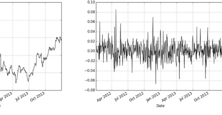
Most raw ﬁnancial data are far from being stationary, but it is possible to apply simple transformations to them in order to obtain WSS time series, the most common being the use of returns instead of prices. As will be seen in section 2.5, it is also useful to favor log returns over "standard" returns.

Figure1shows plots for (a) Apple Inc. stock prices for the years of 2012 and 20133

and (b) their log returns, the ﬁrst being non-stationary and the second being WSS.

3

(21)

(a) AAPL prices (b) AAPL log returns

Figure 1 – Weak-sense stationarity example

1.3 Linear Regression

Econometrics is a field of economics which seeks to find relationships between economic variables by employing methods from statistics, mathematics and computer science. Most of these relationships are studied in the form of linear regressions, because estimating their parameters is relatively easy and yet they are powerful enough to describe how most financial variables relate to each other. All the models presented in this work are linear regressions.

A linear regression models how the value of independent variables aﬀects the value of a dependent variable, having the following general form:

yt=α+β1x1,t+β2x2,t+...+βn−1xn−1,t+βnxn,t+ǫt, (1.3)

or, simply:

yt =α+ n

X

i=0

βixi,t+ǫt, (1.4)

where:

• t represents thetth _{observation of a variable;}

• y is the dependent variable;

• xi are the independent variables;

• α is a parameter representing the intercept;

• βi are parameters representing the weight that the values of each xi have in the

value ofy;

(22)

A well known risk measure in the market is theβ of an investment (a single security or a basket), which relates its returns to the returns of a benchmark, often the market itself. This measure is calculated using a simple linear regression:

rt=α+βrb,t+ǫt, (1.5)

where r is the return of the investment, and rb is the return of the used benchmark.

The noise ǫ may here be interpreted as an unexplained return, and α is the so called active-return of an investment. The investment follows the return of the benchmark by a factor of β, meaning that if the absolute value of this parameter is smaller than one, the investment is less volatile than the benchmark.

A good proxy for the market performance may be given by an index, such as the well known S&P 500. This particular index was used to ﬁnd aβ value of approximately 0.98 for Apple Inc. stocks, using data for the years of 2012 and 2013. Details on how to estimate parameters of linear regressions will be brieﬂy discussed in chapter 3.

1.4 High Frequency Financial Data

With the rise of systems capable of rapid performing automated and algorithmic trading strategies, popularly known as high frequency trading, the amount of data generated during a single trading day is enormous, sometimes in a ratio of a trade every millisecond, for each asset. This quantity of available high frequency intraday information allowed researchers to develop models as the HEAVY model that is studied in this work, because before technology allowed, there were not enough per day data to take advantage from. One of the ﬁrst major publications in the subject is (GENÇAY et al., 2001).

Sometimes, the expression high frequency financial data refers to all the information found in an exchange’s order book, including not only effective trades, but all the bids and asks that occurred during a day. These may also appear in the literature as ultra high frequency financial data and can have many practical applications, but they are not the focus here. A model for the dynamics of the order book applied in the context of HFT was the subject of a dissertation presented by a previous master student from Fundação Getulio Vargas (NUNES,2013) (in Portuguese).

(23)

22

2 Mean Models

Even though volatility models may be applied completely separated from mean models, a good understanding of the latter is a valuable asset when learning them. This chapter aims to give the reader a review on the subject.

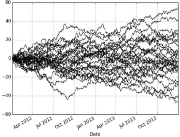
2.1 Random Walk

The most basic way to model the mean is through a random walk. It is a stochastic process where the next value of a variable yt is given by its previous value yt−1 plus a random perturbation. That is:

yt =yt−1+ǫt, ǫt i.i.d.

∼ N(0_,1)_, (2.1)

where ǫt is an independent and identically normally distributed random variable, with

mean 0 and variance 1. An error of this form is also known in the literature as a white noise.

This process is a Markov chain, since it has no memory of older values, other than the last one. It is also a martingale1_{, i.e.} _E₍_y

t+s|Ft) = yt, ∀t, s, so forecasting is

impossible, since the expected value of any future iteration of yt will always be the current

value. Figure 2shows 30 simulations of a random walk process, with y0 = 0, as if it had been observed daily during the years of 2012 and 2013.

Figure 2 – Random walk example

1 _F

(24)

Chapter 2. Mean Models 23

2.2 Autoregressive Models

As its name should already suggest, an autoregressive (AR) model of order p is one of the form:

yt=ω+α1yt−1+α2yt−2+...+αp−1yt−(p−1)+αpyt−p +ǫt, ǫt i.i.d.

∼ N₍₀_,₁₎_, _(2.2)

or, simply:

yt =ω+ p

X

i=1

αiyt−i+ǫt, ǫt i.i.d.

∼ N₍₀_,₁₎_. _(2.3)

An AR(p) is then a model where there is an autoregression of the dependent variableytby itsp past values,yt−1, yt−2, ..., yt−(p−1), yt−p, the independent variables of the

model, with parameters ω, α1, α2, ..., α(p−1), αp.

If the process being modeled is stationary, some conclusions about the possible values of the parametersαi may rise. For simplicity, consider an AR(1) model:

yt=ω+α1yt−1+ǫt, ǫt i.i.d.

∼ N₍₀_,₁₎_. _(2.4)

If the expectation is taken:

E(_y_t) = E(_ω+_α₁_y_t₋₁+_ǫ_t)

=E₍_ω_{) +}E₍_α₁_y_t₋_{1) +}E₍_ǫ_t₎

=E₍_ω_{) +}E₍_α₁₎E₍_y_t₋₁_{) +}E₍_ǫ_t₎

=ω+α1E(yt−1). (2.5)

For the process to be stationary, E₍_y_t_{) must be constant,}_∀_t_:

E₍_y_t_{) =}E₍_y_t₋_{1) =}_{µ ,} _(2.6)

hence,

E₍_y_t₎₋_α₁E₍_y_t₋_{1) =} _µ₍₁₋_α_{1) =} _{ω ,} _(2.7)

and

µ= ω 1₋α1

. (2.8)

That is,α1 6= 1 and, from (2.7), ω =µ(1−α1):

yt=ω+α1yt−1+ǫt

=µ(1₋α1) +α1yt−1+ǫt

=µ₋α1µ+α1yt−1+ǫt, (2.9)

and, ﬁnally,

(25)

Taking the variance from (2.10):

Var(yt) = α21Var(yt−1) + 1. (2.11)

Var(yt) should also be constant, ∀t, such that:

Var(yt) = Var(yt−1) =σ2, (2.12)

hence,

Var(yt)−α2₁Var(yt−1) =σ2(1−α12) = 1, (2.13)

and

σ2 = 1 1₋α2

1

. (2.14)

Since variance is a positive quantity,_|α1|<1.

2.2.1 Forecasting

When using AR(p) models for forecasting, all one needs to do is to calculate the expected value of yt s-steps ahead, s being the horizon of prediction, given the information

available until the moment. The name mean model comes exactly from this seek for the expected value, or the mean.

Forecasting yt+3 using an AR(2) model would be:

E(_y_t₊₃_|F_t_{) =}E(_ω+_α₁_y_t₊₂+_α₂_y_t₊₁+_ǫ_t₊₃_|F_t₎ =ω+α1E(yt+2|Ft) +α2E(yt+1|Ft)

=ω+α1E(ω+α1yt+1+α2yt+ǫt+2|Ft) +α2E(ω+α1yt+α2yt−1+ǫt+1|Ft)

=ω+α1ω+α21E(yt+1|Ft) +α1α2yt+α2ω+α2α1yt+α22yt−1 =ω(1 +α1+α2) + 2α1α2yt+α22yt−1+α21E(yt+1|Ft)

=ω(1 +α1+α2) + 2α1α2yt+α22yt−1+α21E(ω+α1yt+α2yt−1+ǫt+1|Ft)

=ω(1 +α1+α2) + 2α1α2yt+α2₂yt−1+α21ω+α31yt+α2₁α2yt−1

(26)

A possible Python implementation of2.15 is:

import numpy

def ar2_forecast ( omega , alphas , y_past , steps =1):

"""

Returns the ’ steps’−ahead forecast for the AR (2) model .

"""

y = numpy . zeros ( steps + 2)

y [0] = y_past [0]

y [1] = y_past [1]

for i in range(2 , steps + 2):

y[i] = omega + alphas [0] ∗ y[i−1] + alphas [1] ∗ y[i−2]

return numpy . copy (y [2:( steps + 2)])

2.3 Moving Average Models

A moving average (MA) model has a similar structure to an AR model, but instead of using the past values of the dependent variable as the independent variables, it uses the past perturbations. A MA(q) model is of the form:

yt=ω+β1ǫt−1+β2ǫt−2+...+βq−1ǫt−(q−1)+βqǫt−q+ǫt, ǫt i.i.d.

∼ N₍₀_,₁₎_, _(2.16)

or, simply:

yt=ω+ q

X

j=1

βjǫt−j +ǫt, ǫt i.i.d.

∼ N₍₀_,₁₎_. _(2.17)

2.4 Autoregressive Moving Average Models

An autoregressive moving average (ARMA) model is a union of the two previously presented models. An ARMA(p, q) has the following form:

yt=ω+ p

X

i=1

αiyt−i+ q

X

j=1

βjǫt−j+ǫt, ǫt i.i.d.

(27)

2.5 Autoregressive Integrated Moving Average Models

When a stochastic processYt is not WSS, one possible way to transform it in one

is to diﬀerentiate it. That is, instead of modeling yt, ∆1yt is modeled:

∆1_y

1 =yt−yt−1. (2.19)

Two direct implications of this are:

• if ∆1_y

t is stationary and completely random, ∆1yt=ǫt, then yt is a random walk;

• if yt is the log price of an asset, ∆1yt represents its log return (as mentioned in

section 1.2).

An ARIMA(p, d, q) is a model in which the time series is diﬀerentiated d-times before the proper ARMA(p, q) is used. As a consequence, modeling with an ARIMA(p,0, q) is exactly the same as direct applying an ARMA(p, q).

∆d_y

t=ω+ p

X

i=1

αi∆dyt−i+ q

X

j=1

βjǫt−j +ǫt, ǫt i.i.d.

∼ N(0_,1)_. (2.20)

The name autoregressive integrated moving average (ARIMA) comes from the fact that if one has a time series generated by this model, it is necessary to "integrate" it

d-times in order to obtain a series in the same unit as yt.

2.6 ARIMA with Explanatory Variables Models

Finally, an ARIMA with explanatory variables (ARIMAX) is an ARIMA with extra independent variables, which are neither autoregressives nor moving averages:

yt=ω+ p

X

i=1

αiyt−i+ q

X

j=1

βjǫt−j+ n

X

k=1

γxk,t+ǫt, ǫt i.i.d.

∼ N₍₀_,₁₎_, _(2.21)

wherexk are exogenous variables at instantt, which can be any other variable that are

known to somehow relate to y.

Note that in the equation above yt was used instead of ∆dyt. In favor of notation

(28)

27

3 Estimation

Linear regression models were presented in both previous chapters, but until now no word was said about how to ﬁnd the right values for each of the model’s parameters. The focus of this chapter is to give an introduction to two of the most used estimation methods: ordinary least squares and maximum likelihood. A simple AR(1) will be used to exemplify the application of both of them, but extending the idea to a more complex model should not be a problem.

3.1 Ordinary Least Squares

Given an AR(1) model:

∼ N₍₀_,₁₎_, _(3.1)

and reorganizing the equation:

ǫt=yt−ω−α1yt−1. (3.2)

The goal of the Ordinary Least Squares (OLS) method is to ﬁnd the values ˆω and ˆ

α1 for the parametersω and α1, respectively, that minimize the squared errors, given a sample of size T. That is:

argmin

ω,α1

T

X

t=2

ǫ2_t = argmin

ω,α1

T

X

t=2

(yt−ω−α1yt−1)2 = argmin

ω,α1

f(ω, α1). (3.3)

Note that the sum starts by the second element, since values for both yt and yt−1 are needed. The estimated parameters ˆωand ˆα1 will be the solution of the following system of equations:

δf

δωˆ =−2

T

X

t=2

(yt−ωˆ−αˆ1yt−1) = 0 ; (3.4)

δf δαˆ1

=₋2

T

X

t=2

(yt−ωˆ−αˆ1yt−1)yt−1 = 0. (3.5)

Solving (3.3) for ˆω:

−2

T

X

t=2

(yt−ωˆ−αˆ1yt−1) = 0

T

X

t=2

(yt−ωˆ−αˆ1yt−1) = 0

T

X

t=2

yt= T X t=2 ˆ ω+ T X t=2 ˆ

(29)

Chapter 3. Estimation 28

Rewriting:

T

X

t=2

yt= ˆω T

X

t=2

1 + ˆα1

T

X

t=2

yt−1. (3.7)

Now, dividing both sides by (T ₋1):

T

X

t=2

yt

T ₋1 = ˆω

T

X

t=2 1

T ₋1 + ˆα1

T

X

t=2

yt−1

T ₋1. (3.8)

Being ¯x=Pn

i=1 xni (the sample mean), it is possible to simplify (3.8):

¯

yt = ˆω+ ˆα1y¯t−1, (3.9)

and ﬁnally ﬁnd the right value for ˆω:

ˆ

ω= ¯yt−αˆ1y¯t−1. (3.10)

Now, substitute ˆω in (3.3):

argmin

ω,α1

T

X

t=2

[yt−(¯yt−αˆ1y¯t−1)−α1yt−1]2

argmin

ω,α₁ T

X

t=2

[yt−y¯t+ ˆα1y¯t−1−α1yt−1]2

argmin

ω,α1

T

X

t=2

[(yt−y¯t)−αˆ1(yt−1−y¯t−1)]2. (3.11)

Diﬀerentiating and solving for ˆα1:

−2

T

X

t=2

[(yt−y¯t)−αˆ1(yt−1−y¯t−1)](yt−1−y¯t−1) = 0

T

X

t=2

[(yt−y¯t)−αˆ1(yt−1−y¯t−1)](yt−1−y¯t−1) = 0

T

X

t=2

(yt−y¯t)(yt−1−y¯t−1)−αˆ1(yt−1−y¯t−1)2 = 0

ˆ

α1 = PT

t=2(yt−y¯t)(yt−1 −y¯t−1)

(yt−1−y¯t−1)2

= Cov(yt, yt−1) Var(yt−1)

. (3.12)

In section1.3 theβ measure was presented. To estimate its value using the OLS method, it is as simple as doing:

β = Cov(r, rb) Var(rb)

(30)

3.2 Maximum-Likelihood

Given an AR(1) model:

∼ N₍₀_,₁₎_, _(3.14)

and a sample y1, y2, ..., yT−1, yT of size T. If the sample observations are assumed to be

independent and identically distributed, it is known that the joint probability distribution of them is equal to the product of the their individual distributions, given the parameters

ω and α1:

f(y2, ..., yT−1, yT |ω, α1) = f(y2|ω, α1)×...×f(yT−1|ω, α1)×f(yT |ω, α1). (3.15)

Since the presented models assume a distribution for the perturbation term (which is actually unknown), the objective of the maximum-likelihood estimation (MLE) is to ﬁnd parameter values that make the sample distribution match the assumed one. For this, the likelihood function is deﬁned as:

ℓ(ˆω,αˆ1; y2, ..., yT), (3.16)

where ˆω and ˆα1 are variable parameters and y2, ..., yT are ﬁxed parameters. The goal is to

ﬁnd values for ˆω and ˆα1 to which:

ℓ(ˆω,αˆ1; y2, ..., yT) =f(y2, ..., yT |ω, α1) =

T

Y

t=2

f(yt|ω, α1). (3.17)

In order to do that, we maximize ℓ, and that is the reason the method is called maximum-likelihood. Given that all the sample is available, _∀t_≥1:

E₍_y_t_|F_t₋_{1) =}E₍_ω₊_α₁_y_t₋₁₊_ǫ_t_|F_t₋₁₎

=ω+α1yt−1, (3.18)

and

Var(yt|Ft−1) = Var(ω+α1yt−1+ǫt|Ft−1) = 1. (3.19)

Assuming thatǫt is a white noise:

ℓ(ˆω,αˆ1;y2, ..., yT) = T

Y

t=2

f(yt|ω,ˆ αˆ1)

= T Y t=2 1 √

2πexp

"

−(yt−ωˆ −αˆ1yt−1)

2

#

. (3.20)

The MLE estimates ˆω and ˆα1 will be given by:

argmax ˆ

ω,αˆ1

(31)

Since the maximum of a product may be very diﬃcult to solve by hand, and may cause ﬂoating point problems in a computer, it is usual to calculate the maximum of the log-likelihood function. The result is the same, since log is a strictly monotonically increasing function.

argmax ˆ

ω,αˆ1

lnℓ(ˆω,αˆ1;y2, ..., yT) = argmax

ˆ

ω,αˆ1

T X t=2 ln ( 1 √

2π exp

"

−(yt−ωˆ−αˆ1yt−1)

2

#)

= argmax ˆ

ω,αˆ1

T

X

t=2

ln √1

2π

!

−

"

(yt−ωˆ−αˆ1yt−1)2 2

#

= argmax ˆ

ω,αˆ₁

T

X

t=2

ln 1₋ln√2π₋

"

#

= argmax ˆ

ω,αˆ1

T

X

t=2 1

2ln 2π− "

#

= argmax ˆ

ω,αˆ1

T

X

t=2 1

2[ln 2π−(yt−ωˆ−αˆ1yt−1)

2_]_. _(3.22)

The estimated parameters ˆω and ˆα1 will be the solution of the following system of equations:

δf δωˆ =

T

X

t=2

(yt−ωˆ−αˆ1yt−1) = 0 ; (3.23)

δf δαˆ1

=

T

X

t=2

(yt−ωˆ−αˆ1yt−1)yt−1 = 0. (3.24)

Which, in this case, yield exactly the same results as the ones of the OLS method, (3.10) and (3.12).

(32)

Part II

(33)

32

4 GARCH Family

Following the study of mean models, part II focuses completely on volatility models, and this chapter is responsible for introducing the most known and used family of daily volatility models in the market (when one seeks for something more robust than just standard deviations). Afterwards, GARCH models will be used as benchmarks in the tests of chapter 9.

Up until this point, it was assumed that the variable being modeled could be any one. From now on, the text will implicitly assume that the variable of interest is the volatility of returns of a given asset.

4.1 ARCH

Introduced in (ENGLE, 1982), the autoregressive conditional heteroskedasticity (ARCH) model attempts to give a dynamics to the perturbations of the mean models, other than just assuming they are all white noises. A proper deﬁnition of an ARCH of order q is of the following form:

ǫt =σtηt, ηt i.i.d.

∼ N₍₀_,₁₎_, _(4.1)

σ_t2 =ω+α1ǫ2t−1 +α2ǫ2t−2+...+αq−1ǫ2t−(q−1)+αqǫ2t−q. (4.2)

In order to ﬁnd the right parameters to this model, though, it has to be combined with a mean model, like the ones from chapter2, so that ﬁnding values forǫt, ∀t, becomes

feasible. If it is the desire of the user to use it standalone, as it was in this work, one needs to assume the log prices of the underlying asset to be random walks, so that their log returns are given only by:

rt=ǫt. (4.3)

This way, ARCH may be simpliﬁed to:

rt=σtηt, ηt i.i.d.

∼ N(0_,1)_, (4.4)

σ2_t =ω+

q

X

j=1

αjr2t−j, (4.5)

and anyone can use it to model and forecast volatility without properly modeling rt.

If historical price information is available, it is possible to ignore (4.1) completely, using returns to directly model their volatility with (4.5). The sections that follow will assume this is the only goal, and no attention will be given to the possible dynamics rt

(34)

Chapter 4. GARCH Family 33

4.2 GARCH

Although ARCH was the first model of this family, the generalized autoregressive conditional heteroskedasticity (GARCH) (BOLLERSLEV,1986) is the most known one. The main difference from its predecessor is that it employs an AR-like dynamics to the model. A GARCH(p, q) may be specified as:

σ_t2 =ωG+αG,1r2t−1+αG,2rt2−2+...+αG,q−1rt2−(q−1)+αG,qr2t−q

+βG,1σt2−1+βG,2σt2−2 +...+βG,p−1σt2−(p−1)+βG,pσt2−p, (4.6)

or, simply:

σ2_t =ωG+ q

X

j=1

αG,jrt2−j+ p

X

i=1

βG,iσ2t−i. (4.7)

Therefore, in this model, σt2 is a regression of the q past values of r2 plus an

autoregression (AR) of its ownppast values, with parametersωG, αG,1, ..., αG,q, βG,1, ..., βG,p.

The subscripted G will be important later when diﬀerentiating the estimated parameters in the experiments, since the Greek letters ω, α, β are used across all models which will be tested. Choosing diﬀerent letters would probably just cause more confusion, so the subscript will be adopted from now on.

Like it was done before with the AR model, if Rt is supposed to be WSS, it

is possible to ﬁnd restrictions to the possible values of αG,j, βG,i as well. Consider a

GARCH(1,1) model:

σ2_t =ωG+αG,1r2t−1 +βG,1σ2t−1. (4.8)

Taking the expectation ofσ_t2 is the same as taking the variance ofr:

E₍_σ2_t_{) =} E₍_ω_G₊_α_G,₁_r_t2

−1+βG,1σt2−1)

=E(_ω_G) +E(_α_G,₁_r_t2₋₁) +E(_β_G,₁_σ_t2₋₁)

=E(_ω_G) +E(_α_G,₁)E(_r2_t

−1) +E(βG,1)E(σ2t−1)

=ωG+αG,1E(rt2−1) +βG,1E(σ2t−1). (4.9)

From (4.4), it is known thatE(_r_t2) =E(_σ_t2) and, for the process to be stationary, E₍_σ2

t) must be a constant,∀t:

E₍_σ_t2_{) =}E₍_σ_t2

−1) =E(r2t−1) = σ2, (4.10) hence,

E(_σ_t2)₋_α_G,₁E(_r2_t₋₁)₋_β_G,₁E(_σ_t2₋₁) =_σ2(1₋_α_G,₁₋_β_G,₁) =_ω_G_, (4.11)

and

σ2 = ωG 1₋αG,1−βG,1

. (4.12)

(35)

4.2.1 Estimating

For all the models that are going to be used in the experiments of chapter9, the MLE was the method of choice to estimate the parameters. Since GARCH will be used in its GARCH(1,1) form, this will be the example here.

Remember that, the objective of this method is to ﬁnd values for ˆωG, ˆαG,1, and ˆ

βG,1 to which:

ℓ(ˆωG,αˆG,1,βˆG,1;r2, ..., rT) =f(r2, ..., rT |ωG, αG,1, βG,1)

=

T

Y

t=2

f(rt|ωG, αG,1, βG,1). (4.13)

Given that all the sample is available, _∀t_≥1:

E₍_r_t_|F_t₋₁_{) =}E₍_σ_t_η_t_|F_t₋_{1) = 0}_, _(4.14) and

Var(rt|Ft−1) = Var(σtηt|Ft−1)

=E₍_σ_t2_|F_t₋₁₎ =E₍_ω₊_α_G,₁_r2

t−1+βG,1σ2t−1|Ft−1)

=ωG+αG,1rt2−1+βG,1σt2−1. (4.15)

Assuming thatηt is a white noise:

ℓ(ˆωG,αˆG,1,βˆG,1; r2, ..., rT) = T

Y

t=2

f(rt|ωˆG,αˆG,1,βˆG,1), (4.16)

which is equal to:

T

Y

t=2

1 q

2π(ˆωG+ ˆαG,1rt2−1+ ˆβG,1σt2−1) exp

"

− r

2

t

2(ˆωG+ ˆαG,1r2t−1+ ˆβG,1σt2−1) #

. (4.17)

The MLE estimates ˆωG, ˆαG,1, and ˆβG,1 will be given by:

argmax ˆ

ωG,αˆG,1,βˆG,1

ℓ(ˆωG,αˆG,1,βˆG,1; r2, ..., rT). (4.18)

(36)

4.2.2 Forecasting

If one wants to know the probable value σ2_t will have s-steps ahead in the future, as with the AR model, all that is necessary is to calculate its expected value.

Forecasting σ2

t+3 using a GARCH(1,1) model then is:

E(_σ2_t

+3|Ft) = E(ωG+αG,1r2t+2+βG,1σt2+2|Ft)

=ωG+αG,1E(r2t+2|Ft) +βG,1E(σt2+2|Ft)

=ωG+αG,1E(σ2t+2|Ft) +βG,1E(σt2+2|Ft)

=ωG+ (αG,1+βG,1)E(σt2+2|Ft)

=ωG+ (αG,1+βG,1)E(ωG+αG,1rt2+1+βG,1σ2t+1|Ft)

=ωG+ (αG,1+βG,1)[ωG+αG,1E(rt2+1|Ft) +βG,1E(σ2t+1|Ft)]

=ωG+ (αG,1+βG,1)[ωG+αG,1E(σt2+1|Ft) +βG,1E(σ2t+1|Ft)]

=ωG+ (αG,1+βG,1)[ωG+ (αG,1+βG,1)E(σt2+1|Ft)]

=ωG+ωG(αG,1+βG,1) + (αG,1+βG,1)2E(σt2+1|Ft)

=ωG(1 +αG,1+βG,1) + (αG,1+βG,1)2E(σt2+1|Ft)

=ωG(1 +αG,1+βG,1) + (αG,1+βG,1)2E(ωG+αG,1rt2+βG,1σ2t|Ft)

=ωG(1 +αG,1+βG,1) + (αG,1+βG,1)2(ωG+αG,1rt2+βG,1σ2t). (4.19)

Since (αG,1 +βG,1) < 1, σ2t will slowly, but surely, mean revert. The algorithm

to compute such forecast will also be left to be exempliﬁed in subsection 6.1.2, for the HEAVY case. Again, the same method is easily adapted to work with GARCH and the source code is available in annex A.

4.3 IGARCH

The Integrated Generalized Autoregressive Conditional Heteroskedasticity (IGARCH) looks exactly like a standard GARCH:

σ_t2 =ωIG+ q

X

j=1

αIG,jrt2−j+ p

X

i=1

βIG,iσ2t−i, (4.20)

but it is in fact a restricted version of it, where parameters αIG,j and βIG,i sum up to one:

q

X

j=1

αIG,j+ p

X

i=1

βIG,i = 1. (4.21)

(37)

rt, ∀t >0, are the realizations) is not WSS. (NELSON, 1990) shows, however, that for

a GARCH(1,1)-generated process to be strictly stationary, the necessary condition is

E[_ln(_α_G,₁_η2_t +_β_G,₁)]_<0, a weaker condition than E(_α_G,₁_η_t2+_β_G,₁)_<1.

Given (4.21), whenq=p= 1, it is possible to rewrite:

σ_t2 =ωIG+αIG,1rt2−1+ (1−αIG,1)σt2−1. (4.22)

The letters IGwill be used to designate IGARCH parameters.

4.4 GARCH with Explanatory Variables

A GARCH with Explanatory Variables (GARCHX) is to GARCH as ARIMAX is to ARIMA: a GARCH with extra independent variables, which are neither past values of

rt nor of σ2t:

σ2_t =ωGX + q

X

j=1

αGX,jr2t−j + p

X

i=1

βGX,iσt2−i+ n

X

k=1

γGXxk,t. (4.23)

As it will be further seen in chapter9, this model will be specially useful to produce a joint GARCH-HEAVY model, so that one is able to evaluate which of the two is more descriptive of the daily volatility of the security in question. The letters GX will be used to designate GARCHX parameters.

4.5 GJR-GARCH

The idea behind the GARCH extension proposed in (GLOSTEN; JAGANNATHAN; RUNKLE, 1993) is that future increases in the volatility of returns are associated with present falls in asset prices. To capture this statistical leverage eﬀect, the three authors which gave their initials to the name of the GJR-GARCH model propose the following:

σ_t2 =ωGJ R+ q

X

j=1

αGJ R,jrt2−j+ o

X

k=1

γGJ R,kr2t−kIt−k+ p

X

i=1

βGJ R,iσt2−i, (4.24)

with It= 1 if rt<1, and It = 0 otherwise, ∀t. Adding a new term to the equation every

time a negative return occurred in the past, heightening the eﬀect squared returns have in the resulted volatility.

Since it is not possible to predict whether a negative return will happen, when forecasting with an horizon of size s, s >1, the evaluations from chapter9 will assume:

E₍_I_t₊_s_|F_t_{) =}E₍_I_t₊_s₎_≈ 1

2, (4.25)

causing the constraints to this models’ parameters to be slightly diﬀerent from the ones from GARCH. In the GJR-GARCH(1,1,1) case: αGJ R,1+γGJ R,₂ 1 +βGJ R,1

(38)

37

5 Realized Measures

After presenting the most known GARCH models, the concept of realized measures (RM) need to be explained before continuing, because they are in the heart of the HEAVY

models, which are the focus of this work and will be presented in the next chapter.

As GARCH used the daily returns of an asset,rt, as its main source of information,

the respective realized measures, RMt, are what HEAVY utilizes. They are

nonparametric-based estimators of the variance of a security in a day, which, as opposed to r2_t, ignore overnight eﬀects, and sometimes even the variation of the ﬁrst moments of a given day, since these may be regarded as more noisy than the rest of the trading session.

Both (BARNDORFF-NIELSEN; SHEPHARD,2006) and (ANDERSEN; BOLLER-SLEV; DIEBOLD,2002) give a background on the subject, and the idea here is only to present the realized measures that were used during the tests with the HEAVY family of models in this work.

5.1 Realized Variance

The most simply of the realized measures, realized variance (RV), is the given by the sum of intraday squared returns. If pτ is the log price of an asset at instant τ, then:

RMt =RVt= nt

X

τ=1

(pτ −pτ−1)2, (5.1)

where nt is the number of used intraday prices within dayt. As already pointed out in

section 1.1, ∆τ, the interval between each observation, needs to be a constant to allow equal treatment for eachpτ. In this work, a ∆τ of ﬁve minutes (300s) was used. The source

code for the Python implementation of RVt, given a intraday time series ts, follows:

import numpy

import pandas

def realized_variance (ts , delta =300 , base =0):

ts = ts . resample ( rule =(str( delta ) + ’s ’), how =’last ’, fill_method =’pad ’,

base = base )

ts = numpy . diff ( ts )

ts = numpy . power (ts , 2.0)

(39)

Chapter 5. Realized Measures 38

5.2 Multiscale Realized Variance

The microstructure of the market may be very noisy in practice, and there are several studies available that propose estimators to mitigate this eﬀect. Some examples are: pre-averaging (JACOD et al., 2009); realized kernels (BARNDORFF-NIELSEN et al.,

2008); two scale realized variance (ZHANG; MYKLAND; AÏT-SAHALIA, 2005); and its successor, the multiscale realized variance (MSRV), presented in (ZHANG et al., 2006). The latter was chosen given its simplicity of implementation.

Given realized variances of diﬀerent scales, K:

RV_tK = 1

K

nt

X

τ=K+1

(pτ −pτ−K)2. (5.2)

The MSRVt is deﬁned as:

RMt= MSRVt= Mt

X

i=1

αiRVti, (5.3)

where Mt is the quantity of averaged scales, with its optimal value for a sample of size nt

being in the order of O(√nt). The weights αi are deﬁned as:

αi =

12i M2 t   i Mt −

1 2 −

1 2Mt

1₋ 1

M2

t



 , (5.4)

and the MSRV as whole may be implemented as follows:

from numpy . core . umath import floor , subtract

import numpy

import pandas

def multiscale_realized_variance (ts , delta =300 , base =0):

result = 0.0

base = base )

m = int( floor ( numpy . sqrt (len( ts ))))

m2 = numpy . power (m , 2.0)

for i in range(1 , m + 1):

scaled_ts = subtract ( ts [i:len(x)] , x [0:len( ts)−i ]) scaled_ts = numpy . power ( scaled_ts , 2.0)

result += ((sum( scaled_ts ) / i) ∗ 12.0 ∗ (i / m2 )

∗ ((( i / m) − 0.5 − (1.0 / (2.0 ∗ m )))

/ (1.0 − (1.0 / m2 ))))

(40)

5.3 "Realized EWMA"

Normally used to measure daily volatility, the exponentially weighted moving average (EWMA) is a special case of IGARCH(1,1), where ωIG = 0, and has the form:

σ_t2 = (1₋λ)r2_t₋₁+λσ_t2₋₁. (5.5)

However, the name EWMA is commonly associated in the market to a particular implementation of this model, the one from RiskMetricsTM₍_MORGAN_, ₁₉₉₆_{), which sets}

λ = 0.94.

Usually, when employed in high frequency ﬁnancial data, EWMA serves as an estimator to volatility within a day, as opposed to the other realized measures presented until this point, which measure the open-to-close variance of intraday prices. The idea of a "Realized EWMA" is to measure a RV with weights, hoping that the last returns during a day should have more importance to the overall dynamics. As it will be later presented in chapter 9, this measure, even being quite simple to implement, is very representative. In a similar notation to the previous measures:

RMt= EWMAt= (nt−1) nt

X

τ=1

(0.06)(0.94)nt−τ(_p

τ −pτ−1)2. (5.6)

Without the factor (nt−1), this would be the normally employed version of EWMA.

With this factor, the measure is now in the same magnitude ofr2. For this to work properly, though, the weights should also be normalized, as it is shown in the algorithm below:

import numpy

import pandas

def realized_ewma (ts , delta =300 , base =0):

base = base )

ts = numpy . diff ( ts )

ts = numpy . power (ts , 2.0)

weights = 0.06 ∗ numpy . power (0.94 , range(len( ts ) − 1, −1, −1))

weights /= sum( weights )

return sum( weights ∗ ts ∗ (len( ts ) − 1.0))

Here, the Python function range is used "backwards", creating a list with values

(41)

5.4 Subsampling

Another way to diminish the eﬀect of microstructure noise is to average across subsamples. This is achieved by simply changing the start point of the sampling process: instead of counting intervals of size ∆τ from the beginning of the trading day, these intervals begin after a delay of ﬁfteen or thirty seconds (or any other amount of time).

Subsampling is theoretically always beneﬁcial (HANSEN; LUNDE, 2006) and, like the authors of HEAVY did with their RV estimator, it was applied in the three realized measures presented in this chapter. This was done using starting points every thirty seconds, up to four minutes and a half, creating ten diﬀerent subsamples which were then averaged. The values presented for these measures in partIIIalways consider subsampling.

Implementing it is quite easy, as it may be seen from the code bellow. Here,funmay be the name of any function that calculates a RM, given that they all have the same header.

def subsampling (ts , fun , bins =10 , bin_size =30):

result = 0.0

delta = bins ∗ bin_size

for i in range( bins ):

result += fun (ts , delta = delta , base =( i ∗ bin_size ))

return result / bins

5.5 Realized Semivariance

As the GJR-GARCH, presented in section4.5, tries to measure the eﬀect of statisti-cal leverage, section6.4will present an extended version of the HEAVY model which utilizes realized semivariances (RS) with the same intent. These are realized variances that only make use of negative returns (BARNDORFF-NIELSEN; KINNEBROCK; SHEPHARD,

2008), that is:

RSt= nt

X

τ=1

(pτ−pτ−1)2Iτ, (5.7)

with Iτ = 1 if (pτ −pτ−1) < 1, and Iτ = 0 otherwise, ∀τ1. Applying the same in the

multiscale case would be more tricky, since the weights would have to follow a diﬀerent equation. This was not attempted here.

1

(42)

41

6 HEAVY Family

This chapter is, ﬁnally, responsible for presenting the main subject of this work: the HEAVY family of models. The objective is to measure the eﬃciency of this family proposed in (SHEPHARD; SHEPPARD, 2010) as an alternative to GARCH models in the Brazilian market.

The ﬁrst two sections that follow present the models experimented in the original paper, while the last two sections are dedicated to models that were proposed by the original authors as possible extensions to the standard HEAVY. In chapter 9 all four variants will be tested against their GARCH counterparts to check whether they do or do not stand out in this particular market, as well as if the extensions are really worth applying.

6.1 HEAVY

In section4.2, the GARCH(1,1) was presented as1_:

σ2_t =ωG+αGr2t−1 +βGσ2t−1. (6.1)

If all the information until momentt is available, it is known that:

Var(rt+1|FtLF) =σt2+1 =ωG+αGrt2+βGσt2, (αG+βG)<1 , (6.2)

where the superscript LF stands for low frequency, that is, GARCH only makes use of daily information of security prices variation.

The high-frequency-based volatility (HEAVY) models are speciﬁed as:

Var(rt+1|FtHF) = ht+1 =ωH +αHRMt+βHht, βH <1 ; (6.3)

E(_RM_t₊₁_|FHF

t ) = µt+1 =ωRM+αRMRMt+βRMµt, (αRM +βRM)<1, (6.4)

where (6.3) is named HEAVY-r, which models the close-to-close conditional variance (as GARCH does), and (6.4) is named HEAVY-RM, modeling the open-to-close variation.

Note that, now, the superscriptHF is used, fromhighf requency, since this family of models is designed to harness high frequency ﬁnancial data to predict daily asset return volatility. This is accomplished by using one of the realized measures presented in chapter

5 as the main source of information, as opposed to square returns, like GARCH.

1

(43)

Chapter 6. HEAVY Family 42

Another important remark is that if one only needs to do 1-step ahead forecasts, only HEAVY-r is needed, since HEAVY-RM exists only as a companion model for when multistep-ahead predictions are necessary.

As it will be seen in chapter 9, when compared to GARCH, HEAVY models diﬀer especially in:

• they typically estimate smaller values forβ, with ω being really close to zero, so they tend to be a weighted sum of recent realized measures (having more momentum), while GARCH models normally present longer memory;

• they also tend to adjust faster to changes in the level of volatility, like it can be seen in ﬁgure 3(already using Brazilian data for U.S. Dollar future contracts - HEAVY in black, GARCH in gray).

Figure 3 – HEAVY (in black) vs GARCH (in gray) adjustment to volatility changes

When explaining estimation and forecasting in the HEAVY case, the approach will be diﬀerent to that used with GARCH or AR, where mathematical demonstrations were used. Since the methodology employed in the HEAVY model is quite similar the one from its counterpart, here the focus will be in its algorithmic implementation. The heavyr function that appear in the two following subsections has this form:

def heavyr ( omega , alpha , beta , rm_last , h_last ):

h = omega + alpha ∗ rm_last + beta ∗ h_last

Forecasting daily volatility using high frequency financial data

FUNDAÇÃO GETULIO VARGAS

SÃO PAULO SCHOOL OF ECONOMICS

THIAGO WINKLER ALVES

FORECASTING DAILY VOLATILITY USING HIGH

FREQUENCY FINANCIAL DATA

SÃO PAULO

THIAGO WINKLER ALVES

FORECASTING DAILY VOLATILITY USING HIGH

FREQUENCY FINANCIAL DATA

Supervisor:

Prof. Dr. Juan Carlos Ruilova Terán

THIAGO WINKLER ALVES

FORECASTING DAILY VOLATILITY USING HIGH

FREQUENCY FINANCIAL DATA

ACKNOWLEDGEMENTS

ABSTRACT

RESUMO

List of Figures

List of Tables

List of abbreviations and acronyms

Contents

Introduction

14

I Financial Series Modeling

17

II Volatility Models

31

III Application

46

Conclusion

62

Appendix

66

Introduction

Objectives

Organization

Part I

1 General Definitions

1.1 Time Series

1.2 Stationarity

1.3 Linear Regression

1.4 High Frequency Financial Data

2 Mean Models

2.1 Random Walk

2.2 Autoregressive Models

2.2.1

Forecasting

2.3 Moving Average Models

2.4 Autoregressive Moving Average Models

2.5 Autoregressive Integrated Moving Average Models

2.6 ARIMA with Explanatory Variables Models

3 Estimation

3.1 Ordinary Least Squares

3.2 Maximum-Likelihood

Part II

4 GARCH Family

4.1 ARCH

4.2 GARCH

4.2.1

Estimating

4.2.2

Forecasting

4.3 IGARCH

4.4 GARCH with Explanatory Variables

4.5 GJR-GARCH

5 Realized Measures

5.1 Realized Variance

5.2 Multiscale Realized Variance

5.3 "Realized EWMA"

5.4 Subsampling

5.5 Realized Semivariance

6 HEAVY Family

6.1 HEAVY