Forecasting USD-BRL Currency Rate Volatility using
Realized and Implied Volatilities Data
♦
Carlos Heitor Campani1
Assis Gustavo da Silva Durães2
Abstract
This article assesses the impact of exogenous variables in GARCH models, when applied to volatility forecasts for the Brazilian USD-BRL currency market. As exogenous variables, we used the realized variance, based on high frequency data, and the FXVol index, based on market implied volatility data. This is the first study to use the FXVol index and to investigate its effects on Brazilian foreign exchange volatility. The results indicate statistical significance of the supe-riority of the extended models when predicting volatility. We conclude that high frequency data and market implied volatility contain relevant information with respect to USD-BRL currency volatility. These findings are relevant for hedgers, speculators and practitioners in general.
Keywords
Volatility forecasts, Extended GARCH models, Implied volatility indices, Brazilian foreign exchange market
Resumo
Este artigo avalia o impacto de variáveis exógenas nos modelos GARCH, quando aplicado às previsões de volatilidade para o mercado de câmbio brasileiro USD-BRL. Como variáveis exógenas, foram utilizadas a variância realizada, baseada em dados de alta frequência, e o índice FXVol, baseado em dados de volatilidade implícita no mercado. Este é o primeiro es-tudo a utilizar o índice FXVol e a investigar seus efeitos sobre a volatilidade cambial brasileira. Os resultados indicam significância estatística da superioridade dos modelos estendidos ao prever a volatilidade. Concluímos que os dados de alta frequência e a volatilidade implícita do mercado contêm informações relevantes com relação à volatilidade cambial do USD-BRL. Essas descobertas são relevantes para hedgers, especuladores e profissionais em geral.
Esta obra está licenciada com uma Licença Creative Commons Atribuição-Não Comercial 4.0 Internacional. ♦ The author Carlos Heitor Campani thanks the financial support from the Brasilprev Research Chair in
Social Security and from the Brazilian National School of Insurance. 1 Professor of Finance – Universidade Federal do Rio de Janeiro (UFRJ)
Endereço: Rua Pascoal Lemme, 355 - Ilha do Fundão - Cid. Universitária – Rio de Janeiro/RJ – Brasil CEP: 21941-918 – E-mail: [email protected] – http://orcid.org/0000-0003-1896-7837 2 Researcher – Universidade Federal do Rio de Janeiro (UFRJ)
Endereço: Rua Pascoal Lemme, 355 - Ilha do Fundão - Cid. Universitária – Rio de Janeiro/RJ – Brasil CEP: 21941-918 – E-mail: [email protected] – http://orcid.org/0000-0003-4086-7090
Keywords
Previsão de volatilidade. Modelos GARCH. Índices de volatilidade implícita. Mercado de câmbio no Brasil.
JEL Classification
G10. G12. G17.
1. Introduction
It is a well known fact that volatility plays a central role in modern finance theory, whether in assets pricing and valuation, portfolio allocation or risk management, among other areas. To many investors, volatility is a synonym for risk: They have a certain level of risk they can, or are willing to, bear on their portfolios. An accurate forecast of their assets’ volatility and cor-relations is one of the crucial conditions in order to correctly assess those portfolios risk levels.
A volatility model is usually expected to forecast not only the absolute forecast of returns, but the whole density of those future returns. The vo-latility forecasting theme has always been problematic for both academics and practitioners: Unlike other metrics, volatility is not directly observable in the market, what poses an initial problem when assessing a volatility forecasting model performance. Furthermore different users (e.g., traders, risk managers, policy makers or academics) can have different understan-dings of volatility, and those disparities may “arise from differences in how volatility affects their trading strategies, and in how they understand the fundamental mechanism of security valuation in a financial market”. Therefore, we can assume that there is no such absolute better volatility estimation method, since this may differ for different uses.
model, originally presented in Bollerslev (1986), and its subsequent deve-lopments, proved to be fairly robust, becoming very popular among aca-demics and practitioners.
The main objective of this work is to perform an empirical analysis to identify if GARCH family based volatility forecasting models applied to USD-BRL currency can benefit from using exogenous variables, na-mely: implied volatility, represented by the FXVol index calculated by the Brazilian exchange BM&FBovespa; and realized volatility, through intraday high frequency data. In addition to that, we also compare those models performances against more naive volatility estimative techniques, such as historical standard deviation of returns and the exponentially weighted moving average (EWMA) model. The evidence found in this study sup-ports the conclusion that both, implied and realized volatilities, could provide useful information when modelling volatility, at least for the local USD-BRL currency market. The model with these variables outperfor-med, with statistical significance, all other models analyzed in this study, including standard GARCH family models.
The foreign exchange derivatives market in Brazil is growing very fast. According to BM&FBovespa data, derivatives that have Foreign Exchange as underlying asset occupy the second largest position, after interest rate derivatives, in terms of notional value: roughly USD 400 billion, repre-senting 26% of the total market. In spite of this, there is a relatively small presence of studies investigating this asset volatility in local exchange market. In fact, as far as it was possible to verify, unlike studies in North American stocks market, where the VIX is widely used as representative of implied volatility, there are no studies done in Brazil using as implied volatility measure the index calculated by BM&FBovespa. Therefore, we are confident that our work is original and will be relevant not only for other academics, but also for practitioners.
2. Theoretical and Literature Review
forecast has drawn a lot of attention from academics and practitioners through the last decades, fostering the development of several models. Poon and Granger (2001) provide a comprehensive review of several of those studies at the time the paper was published. The authors classify the models in two major families: Time-series volatility forecasting models, which encompasses those models that use historical data to formulate fo-recasts, including auto-regressive models and stochastic volatility models, among others. A second one, called option based volatility forecasting models, are those that use the information embedded in traded options to infer the underlying asset volatility. Nowadays, we could also cite mo-dels based on non-parametric methods, as well as those based on neural networks algorithms, although these models are out of the scope of this article.
2.1. Realized Range
One set of methods to estimate volatilities is based on daily amplitude, or range, as described, for example, in Yang and Zhang (2000) and Bollen and Inder (2002). Those can be defined as the difference between the highest and the lowest natural logarithm prices over a sample interval. For a tra-ding interval 𝑡𝑡, let’s denote 𝑂𝑂𝑡𝑡 as the opening price, 𝐶𝐶𝑡𝑡 as the closing price,
𝐻𝐻𝑡𝑡 as the highest price, and 𝐿𝐿𝑡𝑡 as the lowest price. We can then define:
𝑜𝑜𝑡𝑡 = ln(𝑂𝑂𝑡𝑡) − ln(𝐶𝐶𝑡𝑡−1) (1a) 𝑢𝑢𝑡𝑡 = ln(𝐻𝐻𝑡𝑡) − ln(𝑂𝑂𝑡𝑡) (1b)
𝑑𝑑𝑡𝑡 = ln(𝐿𝐿𝑡𝑡) − ln(𝑂𝑂𝑡𝑡) (1c) 𝑐𝑐𝑡𝑡 = ln(𝐶𝐶𝑡𝑡) − ln(𝑂𝑂𝑡𝑡) (1d)
Parkinson (1980) developed an estimator that is based only in opening, maximum and minimum prices, and can be defined as:
𝜎𝜎(𝑃𝑃𝑃𝑃𝑃𝑃𝑃𝑃),𝑡𝑡2 =(𝑢𝑢𝑡𝑡− 𝑑𝑑𝑡𝑡) 2
4ln2 (2)
Garman and Klass (1980) developed an estimator that they claim to be more efficient than the one developed by Parkinson (1980), which also considers the daily return, as described below:
𝜎𝜎(𝐺𝐺𝐺𝐺),𝑡𝑡2 = 0.511(𝑢𝑢
𝑡𝑡− 𝑑𝑑𝑡𝑡)2− 0.019(𝑟𝑟𝑡𝑡(𝑢𝑢𝑡𝑡+ 𝑑𝑑𝑡𝑡) − 2𝑢𝑢𝑡𝑡𝑑𝑑𝑡𝑡) − 0.383𝑟𝑟𝑡𝑡2 (3)
Both those estimators rely on the assumption that 𝜇𝜇 = 0 , what means
there is no drift in price evolution process. Rogers et al. (1994) presents
an estimator that overcomes this limitation; however, as in Equation 2, it is valid in the case where there are no jumps:
𝜎𝜎(𝑅𝑅𝑅𝑅),𝑡𝑡2 = 𝑢𝑢
𝑡𝑡(𝑢𝑢𝑡𝑡− 𝑐𝑐𝑡𝑡) + 𝑑𝑑𝑡𝑡(𝑑𝑑𝑡𝑡− 𝑐𝑐𝑡𝑡) (4)
Aiming to provide an estimator that overcome both those limitations,
regarding drift 𝜇𝜇 and opening jump, Yang and Zhang (2000) presented an
estimator based on multiple period data, with the following form:
𝜎𝜎(𝑌𝑌𝑌𝑌),𝑡𝑡2 = 𝜎𝜎𝑜𝑜,𝑡𝑡2 + 𝑘𝑘𝜎𝜎𝑐𝑐,𝑡𝑡2 + (1 − 𝑘𝑘)𝜎𝜎(𝑅𝑅𝑅𝑅),𝑡𝑡2 (5)
where 𝜎𝜎(𝑅𝑅𝑅𝑅),𝑡𝑡2 is given in 4, and 𝜎𝜎𝑜𝑜2, 𝜎𝜎𝑐𝑐2 and 𝑘𝑘 are defined as:
. l𝜎𝜎𝑜𝑜,𝑡𝑡2 = (𝑛𝑛 − 1)−1∑𝑡𝑡−𝑛𝑛𝑖𝑖=𝑡𝑡−1(𝑜𝑜𝑖𝑖− 𝑜𝑜̅)2 (6a)
. 𝜎𝜎𝑐𝑐,𝑡𝑡2 = (𝑛𝑛 − 1)−1∑𝑡𝑡−𝑛𝑛𝑖𝑖=𝑡𝑡−1 (𝑐𝑐𝑖𝑖− 𝑐𝑐̅)2 (6b)
. 𝑘𝑘 =1.34+𝑛𝑛+1𝑛𝑛−10.34 (6c)
with . 𝑜𝑜̅ = 𝑛𝑛−1∑𝑡𝑡−𝑛𝑛𝑖𝑖=𝑡𝑡−1 and 𝑜𝑜𝑖𝑖 . 𝑐𝑐̅ = 𝑛𝑛−1∑𝑡𝑡−𝑛𝑛𝑖𝑖=𝑡𝑡−1𝑐𝑐𝑖𝑖.
2.2. Realized Variance
Andersen and Bollerslev (1997) were the first to propose the sum of squa-red intraday returns as an estimator for the actual volatility. We can re-present intraday returns as:
where 𝑃𝑃𝑡𝑡,𝑑𝑑 is the last price observed at timestamp 𝑑𝑑 at date 𝑡𝑡,𝑟𝑟𝑡𝑡,𝑑𝑑 is the
return at date 𝑡𝑡 in the 𝑑𝑑 − 𝑡𝑡ℎ interval, reflecting the price variation from
timestamp 𝑑𝑑 − 1 to 𝑑𝑑, at date 𝑡𝑡. Hence, the realized volatility as a sum of
squared returns (SSR) would be:
. 𝜎𝜎̃(𝑆𝑆𝑆𝑆𝑆𝑆),𝑡𝑡2 = ∑𝐷𝐷𝑑𝑑=1 𝑟𝑟𝑡𝑡,𝑑𝑑2 𝑡𝑡 = 1,2, . . . , 𝑁𝑁 (8)
In their original work, they defined realized variance (. 𝑅𝑅𝑅𝑅) as the sum
of 288 5-minutes squared returns, and found evidence that the perfor-mance of ARCH-based models increases with intraday data being used.
Similar results were presented in Andersen et al. (1999) and Andersen
et al. (2001). It was also pointed that, due to characteristics of financial
time-series, intervals shorter than 5 minutes are usually polluted with serial correlation, consequence of microstructure noisy effects. It was de-termined that a interval between 5 and 30 minutes is generally a good balance between accuracy of the continuous record underlying realized volatility measures, and long enough such that the influences from market
microstructure are not overwhelming (Torben G. Andersen et al. 2001).
In case of markets in which assets negotiation does not occur continuously, such as equities or non-global currencies, how to incorporate overnight re-turn deserves some notes. Hansen and Lunde (2005a) discuss this matter and proposes three different approaches to integrate the overnight returns with trading hours data and obtain a measure of daily integrated variance. The first alternative to integrate the overnight returns would be simply add those to the estimator defined in 13, as below:
. 𝜎𝜎̃(+𝑂𝑂𝑂𝑂),𝑡𝑡2 ≡ 𝑜𝑜
𝑡𝑡2+ 𝜎𝜎̃(𝑆𝑆𝑆𝑆𝑆𝑆),𝑡𝑡2 (9)
where the two terms can be interpreted as estimators of integrated vari-ance, the first one representing the inactive period and the second for the active market period. As highlighted in Hansen and Lunde (2005a), an
ob-vious drawback of this measure is that the squared overnight return, . 𝑜𝑜𝑡𝑡2, is
a noisy estimator for the non-trading hours, similar as . 𝑟𝑟𝑡𝑡2 fails as estimator for the daily integrated variance.
. 𝜎𝜎̃(𝑆𝑆𝑆𝑆𝑆𝑆𝑆𝑆𝑆𝑆),𝑡𝑡2 ≡ 𝜍𝜍̂ ⋅ 𝜎𝜎̃(𝑆𝑆𝑆𝑆𝑆𝑆,𝑡𝑡)2 (10)
This approach was used in several studies, such as Martens (2002),
Koopman et al. (2005) and Hansen and Lunde (2005b). Hansen and
Lunde (2005a) and Martens (2002) propose ways to estimate the factor 𝜍𝜍̂.
To develop the third alternative, Hansen and Lunde (2005a) work on the idea that both previous estimators, 𝜎𝜎̃(+𝑂𝑂𝑂𝑂),𝑡𝑡2 and 𝜎𝜎̃(𝑆𝑆𝑆𝑆𝑆𝑆𝑆𝑆𝑆𝑆),𝑡𝑡2 are linear combi-nations of 𝑜𝑜𝑡𝑡2 and 𝜎𝜎̃(𝑆𝑆𝑆𝑆𝑆𝑆),𝑡𝑡2 , with weights (1,1) and (0, 𝜍𝜍) respectively. Hence, those can be expressed as:
𝜎𝜎̃(𝜛𝜛),𝑡𝑡2 ≡ 𝜛𝜛1𝑜𝑜𝑡𝑡2+ 𝜛𝜛2𝜎𝜎̃(𝑆𝑆𝑆𝑆𝑆𝑆),𝑡𝑡2 (11)
with 𝜛𝜛1 and 𝜛𝜛2 chosen accordingly (for example, minimizing a given error
measure). Hansen and Lunde (2005a) provide a closed-form solution for
those weights 𝜛𝜛 as below:
𝜛𝜛1≡ (1 − 𝜌𝜌)𝜈𝜈𝜈𝜈0
1 and 𝜛𝜛2≡ 𝜌𝜌
𝜈𝜈0
𝜈𝜈2 (12)
where 𝜌𝜌 is a relative importance factor, defined as:
𝜌𝜌 ≡ 𝜈𝜈22𝜂𝜂12− 𝜈𝜈1𝜈𝜈2𝜂𝜂1,2
𝜈𝜈22𝜂𝜂12+ 𝜈𝜈12𝜂𝜂22− 2𝜈𝜈1𝜈𝜈2𝜂𝜂12 (13)
and 𝜈𝜈0≡ 𝐄𝐄(𝜎𝜎̃2), 𝜈𝜈1≡ 𝐄𝐄(𝑜𝑜2), 𝜈𝜈2≡ 𝐄𝐄(𝜎𝜎̃(𝑆𝑆𝑆𝑆𝑆𝑆),𝑡𝑡2 ), 𝜂𝜂12≡ 𝑣𝑣𝑣𝑣𝑣𝑣(𝑜𝑜𝑡𝑡2), 𝜂𝜂22≡ 𝑣𝑣𝑣𝑣𝑣𝑣(𝜎𝜎̃(𝑆𝑆𝑆𝑆𝑆𝑆),𝑡𝑡2 ) and
𝜂𝜂12≡ 𝑐𝑐𝑐𝑐𝑐𝑐(𝑐𝑐𝑡𝑡2, 𝜎𝜎̃(𝑆𝑆𝑆𝑆𝑆𝑆),𝑡𝑡2 ) .
In practice, the authors propose to estimate those parameters through calculating simple sample averages, and can be rewritten as:
. 1𝜈𝜈̂0,𝑡𝑡≡ 𝑛𝑛−1∑𝑡𝑡−𝑛𝑛𝑖𝑖=𝑡𝑡−1 (𝑜𝑜𝑖𝑖2+ 𝜎𝜎̃(𝑆𝑆𝑆𝑆𝑆𝑆),𝑖𝑖2 ) (14a)
. 𝜈𝜈̂1,𝑡𝑡≡ 𝑛𝑛−1∑𝑡𝑡−𝑛𝑛𝑖𝑖=𝑡𝑡−1 𝑜𝑜𝑖𝑖2 (14b)
. 𝜈𝜈̂1,𝑡𝑡 ≡ 𝑛𝑛−1∑𝑡𝑡−𝑛𝑛𝑖𝑖=𝑡𝑡−1𝑜𝑜𝑖𝑖2 (14c)
. 𝜂𝜂̂1,𝑡𝑡2 ≡ 𝑛𝑛−1∑𝑖𝑖=𝑡𝑡−1𝑡𝑡−𝑛𝑛 (𝑜𝑜𝑖𝑖2− 𝜈𝜈̂1,𝑡𝑡)2 (14d)
. 𝜂𝜂̂2,𝑡𝑡2 ≡ 𝑛𝑛−1∑𝑖𝑖=𝑡𝑡−1𝑡𝑡−𝑛𝑛 (𝜎𝜎̃(𝑆𝑆𝑆𝑆𝑆𝑆),𝑖𝑖2 − 𝜈𝜈̂2,𝑡𝑡)2 (14e)
2.3. Autoregressive Conditional Heteroscedastic Family Models
Originally developed by Engle (1982), the Autoregressive Conditional
Heteroscedastic (ARCH) model estimates the conditional variance 𝜎𝜎̂𝑡𝑡2 as
a function of lagged squared past returns 𝑟𝑟𝑡𝑡−𝑖𝑖. We can write an ARCH(𝑞𝑞 )
model as below:
2𝑟𝑟𝑡𝑡 = 𝜇𝜇 + 𝜀𝜀𝑡𝑡 (15a)
𝜀𝜀𝑡𝑡 = √𝜎𝜎𝑡𝑡2 𝑧𝑧𝑡𝑡 (15b)
. 𝜎𝜎𝑡𝑡2= 𝜔𝜔 + ∑𝑞𝑞𝑖𝑖=1𝛼𝛼𝑖𝑖𝜀𝜀𝑡𝑡−𝑖𝑖2 (15c)
where .𝜎𝜎𝑡𝑡2 is the conditional variance; 𝑧𝑧𝑡𝑡 is a sequence of independent and
identically distributed (iid) random variables with mean 0 and variance 1
(often assumed to follow a normal Gaussian or a Student-t distribution); 𝜔𝜔 > 0 and 𝛼𝛼𝑖𝑖 ≥ 0, for all 𝑖𝑖 > 0 , in order to assure that 𝜎𝜎𝑡𝑡 > 0.
Since volatilities series present a high persistence, too many parameters are often needed when building an ARCH model, what might lead to higher estimation errors (Tsay 2005). To overcome this problem, Bollerslev (1986) proposed an extension, known as generalised ARCH (GARCH) model, that according to the author “allows a much more flexible lag
struc-ture”. In GARCH models, conditional variance .𝜎𝜎𝑡𝑡2 is not only a function
of squared past returns, 𝑟𝑟𝑡𝑡−𝑖𝑖2 , but also of previous conditional variances.
Given that 𝑟𝑟𝑡𝑡 and 𝜀𝜀𝑡𝑡 follow Equations 15a and 15b, the GARCH(𝑝𝑝, 𝑞𝑞)
model can be written as:
.... 𝜎𝜎𝑡𝑡2= 𝜔𝜔 + ∑𝑞𝑞𝑖𝑖=1 𝛼𝛼𝑖𝑖𝜀𝜀𝑡𝑡−𝑖𝑖2 + ∑𝑝𝑝𝑗𝑗=1𝛽𝛽𝑗𝑗𝜎𝜎𝑡𝑡−𝑗𝑗2 (16)
where .... 𝜔𝜔 > 0, 𝛼𝛼𝑖𝑖 ≥ 0, 𝛽𝛽𝑗𝑗≥ 0 and ∑𝑖𝑖=1𝑞𝑞 𝛼𝛼𝑖𝑖+ ∑𝑝𝑝𝑗𝑗=1𝛽𝛽𝑗𝑗< 1 . The later
restric-tion implies that the uncondirestric-tional variance of 𝑟𝑟𝑡𝑡 is finite, therefore
ma-king the model to be stationary.
ARCH and GARCH models still lack in handling the asymmetric effects
between positive and negative returns. Glosten et al. (1993) proposed a
model that addresses this issue, through applying a threshold component
to the 𝑟𝑟𝑡𝑡−𝑖𝑖2 term. It is known as GJR model, from the authors names.
.... 𝜎𝜎𝑡𝑡2= 𝜔𝜔 + ∑𝑞𝑞𝑖𝑖=1 (𝛼𝛼𝑖𝑖+ 𝛾𝛾𝑖𝑖𝑁𝑁𝑡𝑡−𝑖𝑖)𝜀𝜀𝑡𝑡−𝑖𝑖2 + ∑𝑝𝑝𝑗𝑗=1 𝛽𝛽𝑗𝑗𝜎𝜎𝑡𝑡−𝑗𝑗2 (17)
where 𝜔𝜔 > 0 , 𝛼𝛼𝑖𝑖, 𝛽𝛽𝑗𝑗 and 𝛾𝛾𝑖𝑖 are non-negative parameters that satisfy similar
conditions as those of GARCH models, and 𝑁𝑁𝑡𝑡−𝑖𝑖 is an indicator for
nega-tives 𝑟𝑟𝑡𝑡−𝑖𝑖, that is:
𝑁𝑁𝑡𝑡−𝑖𝑖 = {1; if𝑟𝑟
𝑡𝑡−𝑖𝑖< 0 0; if𝑟𝑟𝑡𝑡−𝑖𝑖≥ 0
Nelson (1991) proposed another alternative model to capture asymmetric effects of asset returns on volatility processes, the exponential GARCH
model. The eGARCH(𝑝𝑝, 𝑞𝑞) model can be expressed as below:
. ln(𝜎𝜎𝑡𝑡2) = 𝜔𝜔 + ∑𝑞𝑞𝑖𝑖=1 𝛼𝛼𝑖𝑖|𝜀𝜀𝑡𝑡−𝑖𝑖𝜎𝜎|+𝛾𝛾𝑡𝑡−𝑖𝑖𝑖𝑖𝜀𝜀𝑡𝑡−𝑖𝑖+ ∑𝑝𝑝𝑗𝑗=1𝛽𝛽𝑗𝑗ln(𝜎𝜎𝑡𝑡−𝑗𝑗2 ) (18)
One of the advantages when using the eGARCH model is that the coeffi-cients non-negativity restrictions are relaxed, which simplifies the model estimation procedure.
2.4. Implied Volatility
Previous works suggest that implied volatility (IV) can provide accurate
estimators of the underlying asset price volatility. Some authors argue that conditional on observed options prices and a valuation model, the expected IV should represent a market’s best prediction of a given asset future vola-tility, otherwise arbitrage opportunities would emerge (Jorion (1995) and Poon and Granger (2001), to mention two examples). Its forward-looking nature is intuitive and different than historical backward looking models, making it a natural proxy for future volatility. However, the use of IV is subject to a series of definitions that, once incorrectly made, act as pitfalls
that might undermine a model performance, as mentioned in Blair et al.
(2001).
In order to mitigate these potential issues, several works such as Fleming
et al. (1995), Blair et al. (2001), Koopman et al. (2005), Becker et al.
(2006) and Becker et al. (2007), use the data of implied volatility indices.
According to Fleming et al. (1995), the idea of creating a volatility index
In the case of the studies previously mentioned, the index used was VIX, calculated by the Chicago Board Options Exchange (CBOE). The VIX aims to reflect the 30-day expected volatility of the S&P 500 Index em-bedded in options prices. The components of the VIX calculation are near-the-money and next-term puts and calls options, with more than 23 days and less than 37 days to expiration. The detailed methodology for calculating the VIX can be found in CBOE (2014), as well as detailed numerical examples.
In Brazil, the BM&FBovespa exchange created a local index, to reflect the implied volatility present in the foreign exchange market of USD BRL,
denominated FXVol. The index is calculated based on the listed dollar
options contracts, negotiated at BM&FBovespa. It reflects the implied vola-tility for the next 21 working days period, and when the options maturity does not match this period, an interpolation is performed.
The index is calculated using as framework the variance swaps pricing methodology, through a replicating portfolio, and it undertakes no assump-tion regarding a model for opassump-tions pricing, except that the underlying asset price evolves in a diffusive (continuous) process, hence with no jumps.
Therefore, it claims to be model independent. A complete demonstration of
how it is calculated can be found at Dario (2007) and a detailed descrip-tion of the variance swaps methodology can be seen in Dario (2006). The
index FXVol is calculated on a daily basis,but it is expressed in annualized
terms, considering a year with 252 business days.
We have opted not to use another methodology as a proxy for the implied volatility due to several reasons. To the best of our knowledge, there is no other methodology empirically proved to work better in Brazil. Notice
also that the FXVol index is able to capture the volatility smile trend,
which means that it incorporates more realistic caudal probabilities when compared to implied volatilities originated from at-the-money derivatives. Another reason for this choice is that the data is easily available, with no
need for further computations. Finally, the FXVol index methodology is
2.5. Empirical Literature Review
The topic is extremely debated in the international literature. For exam-ple, Poon and Granger (2001) analyzed 93 published papers that assessed the performance of several volatility models through different asset clas-ses. Most of the literature produced on that matter is devoted to stocks market, seconded by exchange rates. In general, the authors concluded that among the analyzed studies, there were evidence in favor of implied vola-tilities based models forecasts, when compared pairwise against historical volatility and GARCH models, including currencies markets. However, the results of combination of forecasts were mixed. Some examples of previous international works discussing GARCH, RV and IV models
fo-recasting power include Christensen and Prabhala (1998), Becker et al.
(2009), Koopman et al. (2005), Mixon (2009), Jorion (1995), Blair et al.
(2001), and Bentes (2015), just to cite a few. The results, in general, go in favor of RV and IV based models.
When it comes to the Brazilian market, there are also several studies on that topic. Andrade and Tabak (2001) investigates the relationship bet-ween USD-BRL exchange rate implied volatility, obtained from a back-ward induction process, using a Garman-Kohlhagen model and options closing prices, and subsequent realized volatility. The authors found strong evidence that IV contains information about future realized volatility, for both realized volatility measures used. Nevertheless, in line with other studies, the authors found also evidence that IV was an upward-biased estimator of future volatility. Moreira and Lemgruber (2004) investigates the use of high frequency data in the estimation of daily and intraday volatility, in order to compute value at risk forecasts for the IBOVESPA. The author concluded that use of intraday data for obtaining forecasts of daily volatility is feasible and it presents good results.
Mota and Fernandes (2004) examine the forecast for Ibovespa volatility comparing those obtained from ARMA models, using Garman-Klass es-timators, with those forecasts obtained from GARCH models, using as benchmark the realized volatility obtained from 15 min intraday data. The authors concluded that those forecasts obtained from GK-ARMA models are in general as good as those obtained from more complex GARCH models. More examples of previous literature in Brazil are Santanda and
Bueno (2008), Woo et al. (2009), Mendes and Accioly (2012), Maciel
(2012), and Vicente et al. (2012).
Perhaps the most related work to this study is Accioly and Mendes (2016): they investigate if the inclusion of realized range variables in GARCH and eGARCH models for the local Brazilian stocks market adds information and improves the volatility forecasts. They used different definitions of realized range on eight different stocks. The authors found evidence in fa-vor of the extended models, bringing information to the volatility process, with significant persistence reduction. We give a step forward working in a different market (foreign exchange) with also the inclusion of the foreign exchange implied volatility index (FXVol) as a forecasting variable.
3. Data and Methodology
3.1. Data
3.1.1. Daily USD-BRL Data
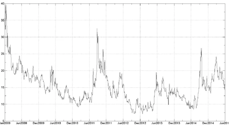
The daily data used in our study consists of USD-BRL currency quotes, where USD is the base currency: In other words, the quotes convention used in this work represents which BRL amount, the quote currency, is equivalent to one unit of USD, the base currency. The period is from January 2nd, 2009 to June 30th, 2015. Given the very low liquidity and, sometimes, absence of data, we had considered only business days in which BM&FBovespa has operated. Also, due to the complete absence of intra-day data on seven intra-days, we have decided to remove these dates from the database as well. In the end, we work with a total of 1,600 trading days.
For each date 𝑡𝑡, four prices were obtained: Open, Close, High and Low
(respectively 𝑂𝑂𝑡𝑡, 𝐶𝐶𝑡𝑡, 𝐻𝐻𝑡𝑡 and 𝐿𝐿𝑡𝑡). Those were captured from Bloomberg da-tabase, ticker <USDBRL Curncy>, PX_OPEN, PX_LAST, PX_HIGH and PX_LOW quotes. Figure 1 illustrates the closing prices evolution through time.
Figure 1 - USD-BRL Currency closing prices: 02Jan2009 - 30Jun2015
3.1.2. Intraday Prices
The intraday data set was obtained from Bloomberg system, using the screen GIT for the same <USDBRL Curncy> ticker used when getting daily data. It consists of USD-BRL quotes with 5-minutes intervals bet-ween 9:00 and 18:00 BRT, encompassing, when a complete daily data set is available, 108 intraday returns observations, and a total 172,601 individual intraday observations: In some dates (242 of the total 1,600), there were some gaps in Bloomberg data, and not all 5-minutes quotes were available. In the cases those gaps occurred between daily first and last quote of the day, we have chosen to interpolate the available data in order to fulfill the gaps. After this procedure, only 28 dates had less than 108 intraday timestamps in our database (days where the first available quote is later than 09:00 or the last one is earlier than 18:00).
The option for the 5-min intervals is based on previous studies, which consider intervals between 5 and 30 minutes as the optimum point that balances the accuracy of the observations with any microstructure pro-blems that can raise from lower frequencies, such as inappropriate
auto-correlation in the series of intraday returns (e.g. Andersen et al. (1999),
Andersen et al. (2001), Martens (2001), Blair et al. (2001), Mota and
Fernandes (2004), Koopman et al. (2005), among several others).
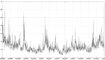
3.1.3. Implied Volatility
The implied volatility data used in this study is the FX Volatility index
(FXVol), calculated by BM&FBovespa and previously described in section
Figure 2 - FXVol Index series: 02Jan2009 - 30Jun2015
The historic series for the index (FXVol) was downloaded from
BM&FBovespa website, from the Information Recovery System. Figure 2 illustrates the evolution of the index for the period we are analyzing. There were eight dates in the period analyzed for which BM&FBovespa did not have the FXVol index information available: We have then decided to linearly interpolate those values using the available data series, in order to fulfill the gaps.
3.2. Analysis of Daily Returns
Figure 3 - USD-BRL Currency daily returns: 02Jan2009 - 30Jun2015
When we perform the augmented Dickey-Fuller test (ADF) in our daily returns database, we have a significant result (p-value: 0.1%; statistic: -43.0585), which supports the stationarity hypothesis of daily returns, as expected.
The autocorrelation (ACF) and partial autocorrelation (PACF) functions
of squared returns series, 𝑟𝑟𝑡𝑡2, indicate relevant serial dependence, as shown
in figure 4, suggesting that the series presents conditional heteroscedastic-ity. Conducting Engle’s test for heteroscedasticity on the residual series (𝜀𝜀𝑡𝑡 = 𝑟𝑟𝑡𝑡− 𝑟𝑟̅), using as alternative hypothesis a 2-lag model, we have a result that strongly rejects the null hypothesis of no ARCH effects on the series, with a statistic value of 174.4, in favor of an ARCH(2) alternative, which supports the adoption of a GARCH(1,1) model in our analysis.
3.3. Realized Volatility
In this section we will describe the steps followed to obtain our estima-tive of realized variance, 𝜎𝜎̃2, and consequently realized volatility, 𝜎𝜎̃ , to be used as an input in our models and as a benchmark to assess those models forecasting accuracy.
Initially, in figure 5 we can see the historical series of the sum of squared intraday returns, 𝜎𝜎̃𝑆𝑆𝑆𝑆𝑆𝑆2 , as described in Equation 8.
Figure 5 - Intraday annualized realized volatility (𝜎𝜎̃(𝑆𝑆𝑆𝑆𝑆𝑆)) series: 02Jan2009 - 30Jun2015
3.4. Models to Be Compared
The first estimate will be simple calculation the standard deviation (SD)
of daily returns, as an estimate for the asset volatility as below:
. 𝜎𝜎̂(𝑆𝑆𝑆𝑆),𝑡𝑡2= (𝑛𝑛 − 1)−1∑𝑛𝑛𝑗𝑗=1 (𝑟𝑟𝑡𝑡−𝑗𝑗− 𝑟𝑟̅𝑡𝑡)2; 𝑟𝑟̅𝑡𝑡= 𝑛𝑛−1∑𝑛𝑛𝑗𝑗=1𝑟𝑟𝑡𝑡−𝑗𝑗 (19)
where . 𝜎𝜎̂(𝑆𝑆𝑆𝑆),𝑡𝑡2 represents the conditional variance forecast for date 𝑡𝑡 and 𝑟𝑟𝑡𝑡
is the daily return as of date 𝑡𝑡. The choice of . 𝑛𝑛 is quite arbitrary, and as
highlighted in Mendes and Duarte (1999), it can impact impact the results obtained. In this work, we compute . 𝜎𝜎̂(𝑆𝑆𝑆𝑆),𝑡𝑡2 , 𝑡𝑡 with a moving window with
the last 20 business days, similar as done in Chang et al. (2002). We had
tested other moving window sizes and, although the results are not pre-cisely the same, they do not impact the overall qualitative results found in this research.
The second estimative will be calculated using an exponentially weighted
moving average (EWMA) forecasting model, as follows:
... 𝜎𝜎̂(𝐸𝐸𝐸𝐸𝐸𝐸𝐸𝐸),𝑡𝑡2 = ∑∞𝑗𝑗=1 [𝑟𝑟𝑡𝑡−𝑗𝑗2 (𝜆𝜆𝑗𝑗−1− 𝜆𝜆𝑗𝑗)] = (1 − 𝜆𝜆)𝑟𝑟𝑡𝑡−12 + 𝜆𝜆𝜎𝜎̂(𝐸𝐸𝐸𝐸𝐸𝐸𝐸𝐸),𝑡𝑡−12 (20)
where ... 𝜆𝜆 will assume the value of 0.94, as commonly used in the literature
such as in Moreira and Lemgruber (2004), among several others.
Similar as Blair et al. (2001), Koopman et al. (2005), Becker et al. (2007)
and Accioly and Mendes (2016), we will use standard GARCH models, including asymmetric returns, realized volatility and implied volatility components on its most comprehensive version. Due to stability pro-blems when estimating models’ coefficients, we had chosen to include the exogenous variables (i.e., implied volatility and realized variance) only in eGARCH model version. The general specification of the models is given as follows:
1𝑟𝑟𝑡𝑡= 𝜇𝜇̂ + 𝜀𝜀𝑡𝑡, 𝜀𝜀𝑡𝑡= 𝜎𝜎̂𝑡𝑡𝑧𝑧𝑡𝑡, 𝑧𝑧𝑡𝑡~𝑁𝑁(0,1) (21a)
𝜎𝜎̂𝑡𝑡2= 𝜔𝜔̂ + (𝛼𝛼̂ + 𝛾𝛾̂𝑁𝑁𝑡𝑡−1)𝜀𝜀𝑡𝑡−12 + 𝛽𝛽̂𝜎𝜎̂𝑡𝑡−12 (21b)
Here 𝑁𝑁𝑡𝑡−1 assumes value of 1 when 𝜀𝜀𝑡𝑡−1< 0 , otherwise is zero; 𝜎𝜎̃𝑡𝑡−12 is the proxy of realized variance, measured from 5-min returns from USD-BRL
currency quotes, as detailed in section 3.3 and 𝐼𝐼𝑉𝑉𝑡𝑡−1 corresponds to the
daily implied volatility index, obtained from annualized FXVol volatility
index.
Equation 21b represents the first two models we will estimate:
I. A GARCH(1,1) model, (GARCH): 𝛾𝛾 = 0.
II. A GJR(1,1) model, (GJR).
Through placing constraints on Equation 21c coefficients, we can represent the remaining 4 variance models we will estimate, as described below:
III. An eGARCH(1,1) model (eGARCH): 𝛿𝛿 = 𝜑𝜑 = 0.
IV. An eGARCH model that includes realized variance as an
exoge-nous variable (eGARCH + RV ): 𝜑𝜑 = 0
V. An eGARCH model that includes implied volatility as an
exoge-nous variable (eGARCH + IV): 𝛿𝛿 = 0
VI. An unrestricted model, that considers both, realized variance and implied volatility, simultaneously (eGARCH + RV+ IV ).
The general parameter vectors 𝜓𝜓𝑘𝑘,𝑡𝑡, for each 𝑘𝑘 model at date 𝑡𝑡, is
𝜔𝜔, 𝛼𝛼, 𝛽𝛽, 𝛾𝛾, 𝛿𝛿, 𝜑𝜑, and those are estimated by maximum likelihood
methodo-logy, using the R software and the rugarch package, which is documented
at Ghalanos (2018).
3.5. Forecasting
Following the same criteria as in Koopman et al. (2005), the forecasting
study is carried based on a rolling window procedure. In each case, the volatility models presented in section 3.4 are estimated 400 times, based on 400 different samples of 1,200 days of observations.
for November 14th, 2013. The second sample starts on January 3rd, 2009 and goes up to November 14th, 2013, such that a forecast is generated for November 18th, 2013 (next business day in Brazil), and so on.
The volatility forecasting evaluation process is an important matter to
determine whether a model 𝑘𝑘 is superior to other. This depends on the
choice of both a proper volatility benchmark and a proper comparison criterion, which are not obvious tasks. In the next subsections we discuss these two issues.
3.6. Volatility Benchmark
Volatility is not directly observable. Consequently, any forecasting error is not observable as well. As we have seen, in several works, the realized variance obtained from intraday returns is often assumed to be an appro-priate proxy for the latent volatility process.
In this study, we will consider the realized volatility as the squared root of the realized variance, as detailed in section 3.3, calculated using the
squared returns of 5-minutes intervals as our proxy for volatility in model
parameter estimation, when applicable, and as our benchmark for model evaluation purposes.
As a robustness exercise, similar to the one performed in Benavides and Capistrán (2012), we will run the evaluation process using, as an alterna-tive benchmark, the estimator proposed in Yang and Zhang (2000) that uses daily range information and is described in section 2.1, Equation 5.
3.7. Comparison Criterion
Several evaluation criteria can be chosen to assess the predictive power or accuracy of a volatility model, and each one is subject to discussion. It is not obvious, as seen in several studies (e.g., Bollerslev et al. (1994) and
Hansen and Lunde (2005b)), which loss function L would be more
Bollerslev et al. (1994) criticizes the widespread use of mean squared er-rors, arguing that it would not properly penalize a given method that pro-vides estimates of zero or even negative volatilities, which are clearly mis-leading and unacceptable. To mitigate this issue, the authors suggest the use of squared percentage errors, absolute percentage error or even the loss function implicit in the Gaussian likelihood, known as Quasi-Likelihood. On the other hand, Koopman et al. (2005) argues that measures like root mean squared percentage errors and mean absolute percentage errors at-tribute relatively less weight to forecast errors associated with high values of realized volatility, when compared to root mean squared error or mean absolute errors. Hence, both of these statistics groups are of interest on their own characteristics. For example, in case of value-at-risk applications, one may be more interested in higher volatility scenarios forecast accuracy than under lower volatility conditions.
Therefore, rather than making a single choice, we will use all the following loss functions in our analysis:
Root Mean Squared Errors (RMSE): 𝐿𝐿1,𝑘𝑘,𝑡𝑡 ≡ √𝑛𝑛−1∑
𝑛𝑛
𝑡𝑡=1
(𝜎𝜎̃𝑡𝑡2− 𝜎𝜎̂𝑘𝑘,𝑡𝑡2 )2
Mean Absolute Errors (MAE): 𝐿𝐿2,𝑘𝑘,𝑡𝑡≡ 𝑛𝑛−1∑
𝑛𝑛
𝑡𝑡=1
|𝜎𝜎̃𝑡𝑡2− 𝜎𝜎̂𝑘𝑘,𝑡𝑡2 |
Root Mean Squared Percentage
Errors (RMSPE):
𝐿𝐿3,𝑘𝑘≡ √𝑛𝑛−1∑
𝑛𝑛
𝑡𝑡=1
(1 − 𝜎𝜎̃𝑡𝑡−2𝜎𝜎̂𝑘𝑘,𝑡𝑡2 )2
Mean Absolute Errors (MAE): 𝐿𝐿4,𝑘𝑘≡ 𝑛𝑛−1∑ 𝑛𝑛
𝑡𝑡=1
|1 − 𝜎𝜎̃𝑡𝑡−2𝜎𝜎̂𝑘𝑘,𝑡𝑡2 |
Median Absolute Percentage 𝐿𝐿5,𝑘𝑘≡(𝑛𝑛 + 1)
2
𝑡𝑡ℎ
termfrom |1 −𝜎𝜎̂𝑘𝑘,𝑡𝑡2
𝜎𝜎̃𝑡𝑡2| term from
𝐿𝐿5,𝑘𝑘 ≡(𝑛𝑛 + 1)2
𝑡𝑡ℎ
termfrom |1 −𝜎𝜎̂𝜎𝜎̃𝑘𝑘,𝑡𝑡2
𝑡𝑡2|
Finally, in order to perform a pairwise comparison between the forecasts and identify which model produces best out-of-sample results, we pro-pose, based on Accioly and Mendes (2016), to use a statistic presented in the seminal work of Diebold and Mariano (1995), which aims to compare predictive accuracy, and we briefly describe it below.
Let’s assume we have two 𝜎𝜎̂𝑡𝑡2 competing models, 𝑖𝑖 and 𝑗𝑗 . Hence, the h-step
ahead forecast errors for the two models on a given forecast date 𝑡𝑡 are:1
𝜀𝜀𝑘𝑘,𝑡𝑡+ℎ|𝑡𝑡 = 𝜎𝜎̃𝑡𝑡+ℎ2 − 𝜎𝜎̂𝑘𝑘,𝑡𝑡+ℎ|𝑡𝑡2 , ; 𝑘𝑘 = 𝑖𝑖, 𝑗𝑗 (22)
It is assumed that the loss associated with a given model 𝑘𝑘 forecast is a
function 𝑔𝑔(𝜀𝜀𝑘𝑘,𝑡𝑡), such as it (1) assumes value zero when no error occur; (2)
is never negative and (3) must necessarily have a positive relation with
er-rors. Typically, 𝑔𝑔(⋅) is the square or the absolute value of errors, and both
those functions will be used in our study.
To determine if a given model predicts better than another, we may test the null hypothesis:
𝐻𝐻0: 𝐸𝐸[𝑔𝑔(𝜀𝜀𝑖𝑖,𝑡𝑡+ℎ|𝑡𝑡)] = 𝐸𝐸[𝑔𝑔(𝜀𝜀𝑗𝑗,𝑡𝑡+ℎ|𝑡𝑡)] (23)
against the alternative hypothesis:
𝐻𝐻1: 𝐸𝐸[𝑔𝑔(𝜀𝜀𝑖𝑖,𝑡𝑡+ℎ|𝑡𝑡)] ≠ 𝐸𝐸[𝑔𝑔(𝜀𝜀𝑗𝑗,𝑡𝑡+ℎ|𝑡𝑡)] (24)
The loss differential between forecasts 𝑖𝑖 and 𝑗𝑗 at time 𝑡𝑡 can be written as
𝑔𝑔(𝜀𝜀𝑖𝑖,𝑡𝑡+ℎ|𝑡𝑡) − 𝑔𝑔(𝜀𝜀𝑗𝑗,𝑡𝑡+ℎ|𝑡𝑡). Hence, in other words, the null hypothesis of equal predictive accuracy can be represented as:
𝐻𝐻0: 𝐸𝐸[𝑑𝑑𝑖𝑖𝑖𝑖,𝑡𝑡] = 0 (25)
The Diebold-Mariano test statistic 𝑆𝑆 is then obtained from:
𝑆𝑆
𝑖𝑖𝑖𝑖 = 𝑑𝑑̅𝑖𝑖𝑖𝑖
√(
𝐿𝐿𝐿𝐿𝑉𝑉̂
𝑑𝑑̅𝑖𝑖𝑖𝑖/𝑛𝑛)
→ 𝑁𝑁(0,1) N(0,1) (26)
where .. 𝑑𝑑̅𝑖𝑖𝑖𝑖= 𝑛𝑛−1∑𝑛𝑛𝑡𝑡=𝑡𝑡0𝑑𝑑𝑖𝑖𝑖𝑖,𝑡𝑡, n stands for the number of loss differential observations and .. 𝐿𝐿𝐿𝐿𝑉𝑉̂𝑑𝑑̅𝑖𝑖𝑖𝑖 represents a consistent estimate for the long-run variance of 𝑑𝑑̅𝑖𝑖𝑖𝑖.
4. Results and Discussion
4.1. In-Sample Results
Table 1 presents the estimated parameters values, p-values, log-likelihoods (lnL), Akaike information criterion (AIC) and Bayesian information crite-rion (BIC) for the models defined in section 3.4. Those results are based on observations for the full sample period, based on 6.5 years of data, between January 2nd, 2009 and June 30th, 2015. It comprises 1,600 daily return observations.
Some conclusions can be drawn from those results. Volatility persistence for all models are estimated as being significant and close to the
uni-ty. For example, in GARCH model we have 𝛼𝛼̂ + 𝛽𝛽̂ = 0.9913 and in GJR
model 𝛼𝛼̂ + 𝛽𝛽̂ + 𝛾𝛾̂/2 = 0.9890 , confirming earlier findings in literature,
such as seen in Koopman et al. (2005), Blair et al. (2001), Accioly and Mendes(2016), among others.
Another interesting observation is related to the non-linearity parameters,
𝛾𝛾̂, on GJR and eGARCH models. As we can see, those are significant
even at a 1% significance level in all cases, and 𝛾𝛾̂ has relevant values, when
compared to 𝛼𝛼̂, suggesting substantial asymmetric affects of returns on
variance. Also, as we can see in Table 1, two of the expanded models pro-posed, 𝑒𝑒𝑒𝑒𝑒𝑒𝑒𝑒𝑒𝑒𝑒𝑒 + 𝑒𝑒𝑅𝑅 and 𝑒𝑒𝑒𝑒𝑒𝑒𝑒𝑒𝑒𝑒𝑒𝑒 + 𝐼𝐼𝑅𝑅 , present significant coefficients at
a 10% significance level on the exogenous variables, 𝛿𝛿̂ and 𝜑𝜑̂, while in the
unrestricted model, 𝑒𝑒𝑒𝑒𝑒𝑒𝑒𝑒𝑒𝑒𝑒𝑒 + 𝑒𝑒𝑅𝑅 + 𝐼𝐼𝑅𝑅 , both exogenous variables
coef-ficients are not significant at a 10% significance level.
When we look at our loglikelihood criterion, we can observe that the unrestricted model presents the best figure, as expected, given that this model is a generalization of the other eGARCH models. However, when
we look the other two criteria, AIC and BIC , we can see an advantage to
Table 1- Models parameters estimation results using the USD-BRL Currency dataset for the period 02 January 2009 to 30 Jun 2015 (1,600 observations)
The complete models specification is: 𝜎𝜎̂𝑡𝑡2= 𝜔𝜔̂ + (𝛼𝛼̂ + 𝛾𝛾̂𝑁𝑁𝑡𝑡−1)𝜀𝜀𝑡𝑡−12 + 𝛽𝛽̂𝜎𝜎̂𝑡𝑡−12 , for models I and II, and
ln(𝜎𝜎̂𝑡𝑡2) = 𝜔𝜔̂ + 𝛼𝛼̂[(|𝜀𝜀𝑡𝑡−1| + 𝛾𝛾̂𝜀𝜀𝑡𝑡−1)/𝜎𝜎̂𝑡𝑡−1] + 𝛽𝛽̂ln(𝜎𝜎̂𝑡𝑡−12 ) + 𝛿𝛿̂ln(𝜎𝜎̃𝑡𝑡−12 ) + 𝜑𝜑̂ln(𝐼𝐼𝑉𝑉𝑡𝑡−12 ) for the remaining models. Parameters estimates we report together with p-values in parenthesis. Those were estima ted maximiz-ing the log likelihood function. The Akaike information criterion (AIC) is calculated as −2 ∗ (ln𝐿𝐿) + 2𝑝𝑝 , where𝑝𝑝is the number of parameters estimated in each model (Akaike 1974). The Bayesian informa-tion criterion (BIC), proposed in Schwarz (1978), is calculated as −2(ln𝐿𝐿) + 𝑝𝑝(ln𝑁𝑁), where 𝑁𝑁 is the sample size. Further discussion on AIC and BIC can be found in Tsay (2005). Numbers in bold indicate statistical significance at the 10% significance level.
4.2. Out-of-Sample Analysis
In the out-of-sample analysis, we compare one day ahead volatility
fore-casts, 𝜎𝜎̂𝑘𝑘, against the benchmarks as previously described in section 3.7,
for the period between November 14th, 2013 to June 30th, 2015. Given the lack of previous studies covering both the same asset and the same me-trics used in this work, it is difficult to be categorical about the results in absolute terms or even to compare the loss functions figures against other studies. Therefore, all comparisons and analysis will be made in relative terms, among the models built here.
Tables 2 and 3 presents the forecasts accuracy figures, introduced in
sec-tion 3.7, using 𝜎𝜎̃ and 𝜎𝜎𝑌𝑌𝑌𝑌 as benchmarks, respectively. Each table contains
loss functions numbers calculated, as previously described. The following five columns ranks each one of the models performance on each criterion separately, from 1 being the best to 8, as the worst performer given a specific criterion. The next two columns consolidate the ranks previously
calculated, summing the relative positions, Sum of Rankings, and ranking
these summation results in the Final Ranking column. As a robustness
check, we also calculated the z-scores for each model loss function re-sult, given each loss function sample average and standard deviation, and obtained an average of those z-scores. The resulting ranking from those
averages is similar to the one presented in column Final Ranking in both
cases, without any significant change.
We can observe in Table 2 that, in terms of RMSPE and MAPE, EWMA
and historical SD models present the best performance when compared
to the GARCH models for this sample, with the 𝑒𝑒𝑒𝑒𝑒𝑒𝑒𝑒𝑒𝑒𝑒𝑒 + 𝑒𝑒𝑅𝑅 + 𝐼𝐼𝑅𝑅 being the third top performer. However, when assessing their performance
through all other criteria, the unrestricted model, 𝑒𝑒𝑒𝑒𝑒𝑒𝑒𝑒𝑒𝑒𝑒𝑒 + 𝑒𝑒𝑅𝑅 + 𝐼𝐼𝑅𝑅 ,
and 𝑒𝑒𝑒𝑒𝑒𝑒𝑒𝑒𝑒𝑒𝑒𝑒 + 𝑒𝑒𝑅𝑅 outperform all other models. In fact, based on the
overall ranking shown in last column, 𝑒𝑒𝑒𝑒𝑒𝑒𝑒𝑒𝑒𝑒𝑒𝑒 + 𝑒𝑒𝑅𝑅 + 𝐼𝐼𝑅𝑅 is the model that presents the most consistent performance, for the sample period analyzed,
followed by 𝑒𝑒𝑒𝑒𝑒𝑒𝑒𝑒𝑒𝑒𝑒𝑒 + 𝐼𝐼𝑅𝑅 and EWMA models.
When using the realized range, 𝜎𝜎𝑌𝑌𝑌𝑌, as benchmark, a slightly
diffe-rent scenario is observed. Once again, our top performer is still model 𝑒𝑒𝑒𝑒𝑒𝑒𝑒𝑒𝑒𝑒𝑒𝑒 + 𝑒𝑒𝑅𝑅 + 𝐼𝐼𝑅𝑅 , however it is seconded now by models 𝑒𝑒𝑒𝑒𝑒𝑒𝑒𝑒𝑒𝑒𝑒𝑒 + 𝐼𝐼𝑅𝑅 and 𝑒𝑒𝑒𝑒𝑒𝑒𝑒𝑒𝑒𝑒𝑒𝑒 + 𝑒𝑒𝑅𝑅, leaving EWMA behind, as shown in Table 3. In fact,
we can see that EWMA relative performance in this case is much more
irregular, given it was ranked as 7th best in three out of five criteria, and
is among the top performers in the remaining two, MAPE and MdAPE. Irrespectively of the benchmark, one conclusion arises: the inclusion of both exogenous variables improved the performance of all GARCH family models. In fact, as it can be observed from both tables, the three GARCH models are performing, on average, not much better than the simple
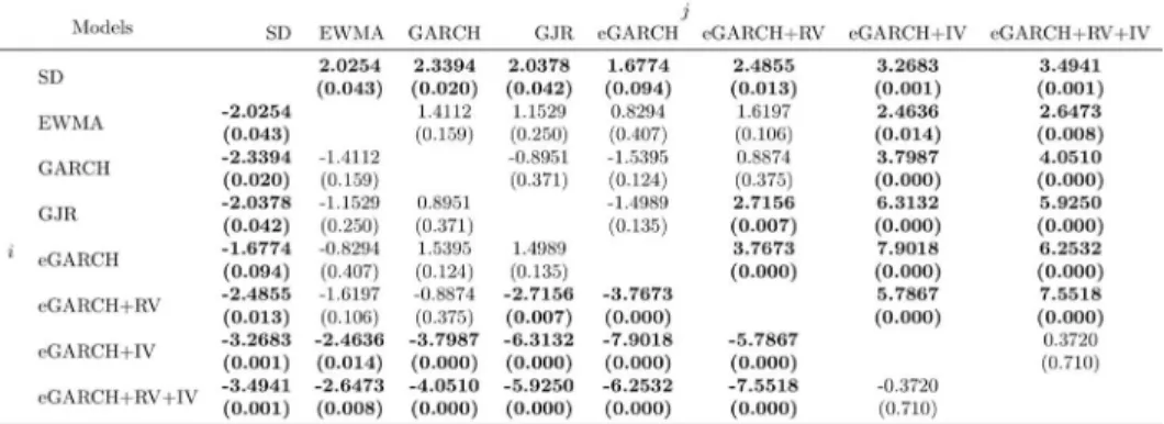
Those results are completely in line with the results of Diebold and Mariano tests shown in Tables 4 and 5. As we can observe, when we
con-sider the squared error as loss function (Table 4), model SD forecasts are
significantly different than all other models, with 10% significance level, being outperformed by all of them. On the other side, we can see model
𝑒𝑒𝑒𝑒𝑒𝑒𝑒𝑒𝑒𝑒𝑒𝑒 + 𝑒𝑒𝑅𝑅 + 𝐼𝐼𝑅𝑅 , which beats all other models at the same significance
level, except for EWMA. Regarding EWMA model, it is worth noticing
that, except for the SD model comparison, it is not possible to reject the
null hypothesis that its errors are, on average, equal to the remaining models, which might undermine its apparent superiority shown in Table 2.
Table 2 - USD-BRL Currency 1-day ahead volatility forecasts, 𝜎𝜎̂𝑘𝑘, comparison against
𝜎𝜎̃ . Evaluation period 14Nov2013 to 30Jun2015 (400 observations)
For a given model 𝑘𝑘, RMSE is defined as . [𝑛𝑛−1∑𝑛𝑛𝑡𝑡=1(𝜎𝜎̃𝑡𝑡2− 𝜎𝜎̂𝑘𝑘,𝑡𝑡2)2] 1/2
, MAE as . 𝑛𝑛−1∑𝑛𝑛𝑡𝑡=1|𝜎𝜎̃𝑡𝑡2− 𝜎𝜎̂𝑘𝑘,𝑡𝑡2|, RMSPE as . [𝑛𝑛−1∑𝑛𝑛
𝑡𝑡=1(1 − 𝜎𝜎̃𝑡𝑡−2𝜎𝜎̂𝑘𝑘,𝑡𝑡2)2] 1/2
, MAPE as
.
𝑛𝑛−1∑𝑛𝑛𝑡𝑡=1|1 − 𝜎𝜎̃𝑡𝑡−2𝜎𝜎̂𝑘𝑘,𝑡𝑡2 | , and MdAPE as the median of . |1 − 𝜎𝜎̃𝑡𝑡−2𝜎𝜎̂𝑘𝑘,𝑡𝑡2|.Table 3 - USD-BRL Currency 1-day ahead volatility forecasts, 𝜎𝜎̂𝑘𝑘, comparison against
. 𝜎𝜎𝑌𝑌𝑌𝑌
. Evaluation period 14Nov2013 to 30Jun2015 (400 observations)For a given model 𝑘𝑘, RMSE is defined as . [𝑛𝑛−1∑𝑛𝑛
𝑡𝑡=1(𝜎𝜎𝑌𝑌𝑍𝑍𝑡𝑡2 − 𝜎𝜎̂𝑘𝑘,𝑡𝑡2)2] 1/2
, MAE as . 𝑛𝑛−1∑𝑛𝑛𝑡𝑡=1|𝜎𝜎𝑌𝑌𝑌𝑌,𝑡𝑡2 − 𝜎𝜎̂𝑘𝑘,𝑡𝑡2|, RMSPE as . [𝑛𝑛−1∑𝑛𝑛
𝑡𝑡=1(1 − 𝜎𝜎𝑌𝑌𝑌𝑌,𝑡𝑡−2𝜎𝜎̂𝑘𝑘,𝑡𝑡2)2] 1/2
, MAPE as . 𝑛𝑛−1∑𝑛𝑛
Table 4 - Diebold and Mariano Test (. ∗and − ) for pairwise comparisons
between volatility forecasts performances (Benchmark: 𝜎𝜎̃ ; . 𝑔𝑔(𝜀𝜀𝑘𝑘) = 𝜀𝜀𝑘𝑘2))
Diebold and Mariano test statistic 𝑆𝑆𝑖𝑖𝑖𝑖 as described in Equation 26. Positive values for 𝑆𝑆𝑖𝑖𝑖𝑖 represent that 𝑔𝑔(𝜀𝜀𝑖𝑖) > 𝑔𝑔(𝜀𝜀𝑗𝑗). In parenthesis, we report the 𝑝𝑝 − 𝑣𝑣𝑣𝑣𝑣𝑣𝑣𝑣𝑣𝑣𝑣𝑣 for a two-tailed Student-t’s test on null
hypothesis 𝐻𝐻0: 𝐸𝐸[𝑔𝑔(𝜀𝜀𝑖𝑖)] = 𝐸𝐸[𝑔𝑔(𝜀𝜀𝑗𝑗)]. Numbers in bold indicate the rejection of null hypothesis at the
10% significance level.
When we analyse the results based on the absolute errors loss function, shown in Table 5, the conclusions are reinforced. Notice that when com-paring SD against GJR and 𝑒𝑒𝑒𝑒𝑒𝑒𝑒𝑒𝑒𝑒𝑒𝑒 + 𝑒𝑒𝑅𝑅, we cannot even reject the null hy-pothesis that those models forecasts are not different from historical stan-dard deviation forecasts. Another change from previous results is that now,
model 𝑒𝑒𝑒𝑒𝑒𝑒𝑒𝑒𝑒𝑒𝑒𝑒 + 𝑒𝑒𝑅𝑅 + 𝐼𝐼𝑅𝑅 is significantly superior even to EWMA model
at a 10% significance level.
When we look at Diebold and Mariano test results using
.
𝜎𝜎
𝑌𝑌𝑌𝑌 and 𝜀𝜀𝑘𝑘2 asloss function, presented in Table 6, we can see a clear superiority of mo-dels 𝑒𝑒𝑒𝑒𝑒𝑒𝑒𝑒𝑒𝑒𝑒𝑒 + 𝑒𝑒𝑅𝑅 + 𝐼𝐼𝑅𝑅 and 𝑒𝑒𝑒𝑒𝑒𝑒𝑒𝑒𝑒𝑒𝑒𝑒 + 𝐼𝐼𝑅𝑅 , since they outperform all other
models. On the other hand, we see again model SD being outperformed,
as well as we can see the poor performance of EWMA model in this
sce-nario. The same results are reinforced when we use |𝜀𝜀𝑘𝑘| as loss function,
as shown in Table 7.
have run the same analysis for forecasts up to 21 days ahead (results available with the authors upon request). The results are in line with the ones presented her, such that the conclusion above remains true (and, in fact, even stronger).
Table 5 - Diebold and Mariano Test(. ∗ and − ) for pairwise comparisons
between volatility forecasts performances (Benchmark: 𝜎𝜎̃ ; 𝑔𝑔(𝜀𝜀𝑘𝑘) = |𝜀𝜀𝑘𝑘|)
Modified Diebold and Mariano test statistic 𝑆𝑆𝑖𝑖𝑖𝑖 as described in Equation 26. Positive values for 𝑆𝑆𝑖𝑖𝑖𝑖 represent that 𝑔𝑔(𝜀𝜀𝑖𝑖) > 𝑔𝑔(𝜀𝜀𝑗𝑗). In parenthesis, we report the 𝑝𝑝 − 𝑣𝑣𝑣𝑣𝑣𝑣𝑣𝑣𝑣𝑣𝑣𝑣 for a two-tailed Student-t’s test on null hypothesis 𝐻𝐻0: 𝐸𝐸[𝑔𝑔(𝜀𝜀𝑖𝑖)] = 𝐸𝐸[𝑔𝑔(𝜀𝜀𝑗𝑗)]. Numbers in bold indicate the rejection of null hypothesis at the 10% significance level.
Table 6 - Diebold and Mariano Test (. ∗and − ) for pairwise comparisons
be-tween volatility forecasts performances (Benchmark:
. 𝜎𝜎
𝑌𝑌𝑌𝑌; . 𝑔𝑔(𝜀𝜀𝑘𝑘) = 𝜀𝜀𝑘𝑘2))Modified Diebold and Mariano test statistic 𝑆𝑆𝑖𝑖𝑖𝑖 as described in Equation 26. Positive values for 𝑆𝑆𝑖𝑖𝑖𝑖 represent that 𝑔𝑔(𝜀𝜀𝑖𝑖) > 𝑔𝑔(𝜀𝜀𝑗𝑗). In parenthesis, we report the 𝑝𝑝 − 𝑣𝑣𝑣𝑣𝑣𝑣𝑣𝑣𝑣𝑣𝑣𝑣 for a two-tailed Student-t’s test
on null hypothesis 𝐻𝐻0: 𝐸𝐸[𝑔𝑔(𝜀𝜀𝑖𝑖)] = 𝐸𝐸[𝑔𝑔(𝜀𝜀𝑗𝑗)]. Numbers in bold indicate the rejection of null hypothesis
Table 7 - Diebold and Mariano Test (. ∗ and − ) for pairwise comparisons
between volatility forecasts performances (Benchmark:
. 𝜎𝜎
𝑌𝑌𝑌𝑌; 𝑔𝑔(𝜀𝜀𝑘𝑘) = |𝜀𝜀𝑘𝑘|)Modified Diebold and Mariano test statistic 𝑆𝑆𝑖𝑖𝑖𝑖 as described in Equation 26. Positive values for 𝑆𝑆𝑖𝑖𝑖𝑖 represent that 𝑔𝑔(𝜀𝜀𝑖𝑖) > 𝑔𝑔(𝜀𝜀𝑗𝑗). In parenthesis, we report the 𝑝𝑝 − 𝑣𝑣𝑣𝑣𝑣𝑣𝑣𝑣𝑣𝑣𝑣𝑣 for a two-tailed Student-t’s test
on null hypothesis 𝐻𝐻0: 𝐸𝐸[𝑔𝑔(𝜀𝜀𝑖𝑖)] = 𝐸𝐸[𝑔𝑔(𝜀𝜀𝑗𝑗)]. Numbers in bold indicate the rejection of null hypothesis
at the 10% significance level.
5. Conclusion
This study investigated the inclusion of exogenous variables in GARCH type models on USD-BRL currency volatility forecasts. More specifically, we included in the standard 𝑒𝑒𝑒𝑒𝑒𝑒𝑒𝑒𝑒𝑒𝑒𝑒 + 𝑒𝑒𝑅𝑅 + 𝐼𝐼𝑅𝑅 model specification two variables:
the USD-BRL Currency implied volatility, IV, represented here by the
FXVol index calculated by BM&FBovespa; and the realized volatility,
𝜎𝜎̃
,obtained from high frequency data. We then assessed the performance of those extended models forecasts against those produced from unmodified models as well as standard models such as historical standard deviation
and the EWMA model.
The evidence found in our study supports the conclusion that both, im-plied and realized volatilities, provide useful information when modelling volatility for the local USD-BRL currency market. The extended models outperformed the standard GARCH models as well as the historical
stan-dard deviation and the EWMA model. This result is robust when using
volatility is the volatility in the past: (expected) future and past seem to be important!
One limitation of this work is related to the studied models’ bias. Hence, this leads to our first suggestion for future research, which would be to in-vestigate the impact of implied volatility and high frequency intraday data on different volatility forecasting models’ specifications, such as regime switching ARCH (SWARCH) or stochastic volatility models, for instance. Another topic for future development relates to the models performance evaluation. One could try to use different frameworks to assess models performance, such as the superior predictive ability (SPA) test, as used in Hansen and Lunde (2005b) and Koopman et al (2005).
Another suggestion for future research is related to the benchmarks used. One could investigate different aspects of realized variance as the proper measure for USD-BRL Currency latent volatility process, such as diffe-rent intraday quotes sampling frequency and microstructure effects, or overnight jumps and what is the best approach to integrate those, as well as investigate alternative sources for the USD-BRL currency data, such as the BM&FBovespa DOL Futures. Regarding the use of the FXVol index as a benchmark for implied volatility, one promising research possibility would be to investigate other methodologies to incorporate the observed volatility smile trend. It is important to remember this is a subject with a wide range of possible approaches, where both worlds, academic and practitioners, certainly have a lot to contribute with. Hopefully, the con-clusions and ideas from this work will concur to the future development of new studies, which will help us to achieve a better understanding of how our local market volatility works, fostering the local development of new products and helping policymakers and, ultimately, the whole society.
References
Akaike, Hiroyuki. 1974. “A New Look at the Statistical Model Identification.” IEEE Transactions on Automatic Control 19 (6): 716–23. https://doi.org/10.1109/TAC.1974.1100705. Accessed on August 22st, 2018
Andersen, T G, Tim Bollerslev, F X Diebold, and Paul Labys. 1999. “The Distribution of Exchange Rate Vo
-latility.” Social Science Research Network 96 (453). Cambridge, MA: 42–55. https://doi.org/10.3386/w6961.
Andersen, Torben G., and Tim Bollerslev. 1997. “Intraday Periodicity and Volatility Persistence in Financial Markets.” Journal of Empirical Finance 4 (2–3). North-Holland: 115–58.
https://doi.org/10.1016/S0927-5398(97)00004-2. Accessed on August 22st, 2018
Andersen, Torben G., Tim Bollerslev, Francis X. Diebold, and Heiko Ebens. 2001. “The Distribution of Realized Stock Return Volatility.” Journal of Financial Economics 61 (1). North-Holland: 43–76. https://doi.org/10.1016/ S0304-405X(01)00055-1. Accessed on August 22st, 2018
Andrade, Sandro Canesso de, Eui Jung Chang, and Benjamin Miranda Tabak. 2002. “Forecasting Exchange Rate Volatility.” In XXIV Encontro Brasileiro de Econometria, 18. Nova Friburgo. http://fmwww.bc.edu/repec/ esFEAM04/up.29425.1077122782.pdf. Accessed on August 22st, 2018
Andrade, Sandro Canesso De, and Benjamin Miranda Tabak. 2001. “Working Paper Series Is It Worth Tracking Dollar/Real Implied Volatility?” Working Paper Series Do Banco Central 1 (fig(15)): 1–25. http://www.bcb.gov. br. Accessed on August 22st, 2018
Becker, Ralf, Adam E. Clements, and Andrew McClelland. 2009. “The Jump Component of S&P 500 Volatility and the VIX Index.” Journal of Banking & Finance 33 (6). North-Holland: 1033–38. https://doi. org/10.1016/J.JBANKFIN.2008.10.015. Accessed on August 22st, 2018
Becker, Ralf, Adam E. Clements, and Scott I. White. 2006. “On the Informational Efficiency of S&P500 Implied Volatility.” The North American Journal of Economics and Finance 17 (2). North-Holland: 139–53. https://doi.org/10.1016/J.NAJEF.2005.10.002. Accessed on August 22st, 2018
———. 2007. “Does Implied Volatility Provide Any Information beyond That Captured in Model-Based Vo
-latility Forecasts?” Journal of Banking & Finance 31 (8). North-Holland: 2535–49. https://doi.org/10.1016/J. JBANKFIN.2006.11.013. Accessed on August 22st, 2018
Bello Accioly, Victor, Beatriz Vaz, and Melo Mendes. 2016. “Assessing the Impact of the Realized Range on the (E)GARCH Volatility: Evidence from Brazil.” Brazilian Business Review 13 (2): 1–26. http://sbfin.org.br/ files/econometria-artigo-xv-ebfin-4855.pdf. Accessed on August 22st, 2018
Benavides, Guillermo, and Carlos Capistrán. 2012. “Forecasting Exchange Rate Volatility: The Superior Perfor
-mance of Conditional Combinations of Time Series and Option Implied Forecasts.” Journal of Empirical Finance 19 (5). North-Holland: 627–39. https://doi.org/10.1016/J.JEMPFIN.2012.07.001. Accessed on August 22st, 2018
Bentes, Sónia R. 2015. “A Comparative Analysis of the Predictive Power of Implied Volatility Indices and GAR
-CH Forecasted Volatility.” Physica A: Statistical Mechanics and Its Applications 424 (April). North-Holland: 105–12. https://doi.org/10.1016/J.PHYSA.2015.01.020. Accessed on August 22st, 2018
Blair, Bevan J., Ser-Huang Poon, and Stephen J. Taylor. 2001. “Forecasting S&P 100 Volatility: The Incre
-mental Information Content of Implied Volatilities and High-Frequency Index Returns.” Journal of Econometrics
105 (1). North-Holland: 5–26. https://doi.org/10.1016/S0304-4076(01)00068-9. Accessed on August 22st, 2018
Bollen, Bernard, and Brett Inder. 2002. “Estimating Daily Volatility in Financial Markets Utilizing Intraday Data.” Journal of Empirical Finance 9 (5). North-Holland: 551–62. https://doi.org/10.1016/S0927-5398(02)00010-5.
Accessed on August 22st, 2018
Bollerslev, Tim. 1986. “Generalized Autoregressive Conditional Heteroskedasticity.” Journal of Econometrics
31 (3). North-Holland: 307–27. https://doi.org/10.1016/0304-4076(86)90063-1. Accessed on August 22st, 2018
Bollerslev, Tim, Robert F. Engle, and Daniel B. Nelson. 1994. “Arch Models.” In Handbook of Econometrics, 4:2959–3038. Elsevier. https://doi.org/10.1016/S1573-4412(05)80018-2. Accessed on August 22st, 2018 CBOE. 2014. “The CBOE Volatility Index - VIX ® The Powerful and Flexible Trading and Risk Managment Tool from the Chicago Board Options Exchange.” Chicago. https://www.cboe.com/micro/vix/vixwhite.pdf.
Accessed on August 22st, 2018
Christensen, B.J., and N.R. Prabhala. 1998. “The Relation between Implied and Realized Volatility.” Journal
of Financial Economics 50 (2). North-Holland: 125–50. https://doi.org/10.1016/S0304-405X(98)00034-8. Ac
Clark, Todd, and Michael McCracken. 2013. “Advances in Forecast Evaluation.” In Handbook of Economic Forecasting, 2:1107–1201. Elsevier. https://doi.org/10.1016/B978-0-444-62731-5.00020-8. Accessed on August
22st, 2018
Diebold, Francis X. 2015. “Comparing Predictive Accuracy, Twenty Years Later: A Personal Perspective on the Use and Abuse of Diebold–Mariano Tests.” Journal of Business & Economic Statistics 33 (1). Taylor & Francis:
1–24. https://doi.org/10.1080/07350015.2014.983236. Accessed on August 22st, 2018
Diebold, Francis X., and Roberto S. Mariano. 1995. “Comparing Predictive Accuracy.” Journal of Business & Economic Statistics 13 (3): 253–63. https://doi.org/10.1080/07350015.1995.10524599. Accessed on August
22st, 2018
Engle, Robert F. 1982. “Autoregressive Conditional Heteroscedasticity with Estimates of the Variance of United Kingdom Inflation.” Econometrica 50 (4). The Econometric Society: 987–1007. https://doi.org/10.2307/1912773.
Accessed on August 22st, 2018
Fleming, Jeff, Barbara Ostdiek, and Robert E. Whaley. 1995. “Predicting Stock Market Volatility: A New Mea
-sure.” Journal of Futures Markets 15 (3). Wiley-Blackwell: 265–302. https://doi.org/10.1002/fut.3990150303.
Accessed on August 22st, 2018
Garman, M., and M. Klass. 1980. “On the Estimation of Security Price Volatilities from Historical Data.” The Journal of Business 53 (1). The University of Chicago Press: 67–68. https://doi.org/10.1086/296072. Accessed
on August 22st, 2018
Genaro, Alan De Dario. 2006. “Apreçamento de Ativos Referenciados Em Volatilidade.” Revista Brasileira de Finanças 4 (2): 203–28. http://bibliotecadigital.fgv.br/ojs/index.php/rbfin/article/viewFile/1162/363. Accessed
on August 22st, 2018
———. 2007. “Índice de Volatilidade Para o Mercado Brasileiro de câMbio: FXvol.” Resenha BM&F 172: 68–76. Ghalanos, Alexios. 2018. “Package ‘Rugarch.’” CRAN-R Project. https://cran.r-project.org/web/packages/rugarch/ rugarch.pdf. Accessed on August 22st, 2018
Glosten, Lawrence, Ravi Jagannathan, and David Runkle. 1993. “On the Relation between the Expected Value
and the Volatility of the Nominal Excess Return on Stocks.” TheJournal of Finance 48 (5). Wiley/Blackwell
(10.1111): 1779–1801. https://doi.org/10.1111/j.1540-6261.1993.tb05128.x. Accessed on August 22st, 2018 Granger, Clive W. J., and Ser-Huang Poon. 2001. “Forecasting Financial Market Volatility: A Review.” Journal of Economic Literature 41 (June): 478–539. https://doi.org/10.2139/SSRN.268866. Accessed on August 22st, 2018
Hansen, Peter Reinhard, and Asger Lunde. 2005a. “A Realized Variance for the Whole Day Based on Intermit
-tent High-Frequency Data.” Journal of Financial Econometrics 3 (4): 525–54. https://doi.org/10.1093/jjfinec/ nbi028. Accessed on August 22st, 2018
———. 2005b. “A Forecast Comparison of Volatility Models: Does Anything Beat a GARCH(1,1)?” Journal of Applied Econometrics 20 (7). Wiley-Blackwell: 873–89. https://doi.org/10.1002/jae.800. Accessed on August
22st, 2018
Jorion, Philippe. 1995. “Predicting Volatility in the Foreign Exchange Market.” The Journal of Finance 50 (2). WileyAmerican Finance Association: 507–28. https://doi.org/10.2307/2329417. Accessed on August 22st, 2018 Koopman, Siem Jan, Borus Jungbacker, and Eugenie Hol. 2005. “Forecasting Daily Variability of the S&P 100 Stock Index Using Historical, Realised and Implied Volatility Measurements.” Journal of Empirical Finance 12 (3). North-Holland: 445–75. https://doi.org/10.1016/J.JEMPFIN.2004.04.009. Accessed on August 22st, 2018
Maciel, Leandro. 2012. “A Hybrid Fuzzy GJR-GARCH Modeling Approach for Stock Market Volatility Forecast
-ing.” Brazilian Review of Finance 10 (3). Sociedade Brasileira de Finanças: 337–67. http://bibliotecadigital.fgv. br/ojs/index.php/rbfin/article/view/3871. Accessed on August 22st, 2018
Martens, Martin. 2001. “Forecasting Daily Exchange Rate Volatility Using Intraday Returns.” Journal of Inter
-national Money and Finance 20 (1). Pergamon: 1–23. https://doi.org/10.1016/S0261-5606(00)00047-4. Accessed