The hydrological response of the Ourthe catchment to climate change as modelled by the HBV model

(1)

HESSD

6, 7143–7178, 2009

The hydrological response of the Ourthe catchment to

climate change

T. L. A. Driessen et al.

Title Page

Abstract Introduction

Conclusions References

Tables Figures

◭ ◮

Back Close

Full Screen / Esc

Printer-friendly Version

Interactive Discussion

Hydrol. Earth Syst. Sci. Discuss., 6, 7143–7178, 2009 www.hydrol-earth-syst-sci-discuss.net/6/7143/2009/ © Author(s) 2009. This work is distributed under the Creative Commons Attribution 3.0 License.

Hydrology and Earth System Sciences Discussions

This discussion paper is/has been under review for the journal Hydrology and Earth System Sciences (HESS). Please refer to the corresponding final paper in HESS if available.

The hydrological response of the Ourthe

catchment to climate change as modelled

by the HBV model

T. L. A. Driessen, R. T. W. L. Hurkmans, W. Terink, P. Hazenberg, P. J. J. F. Torfs, and R. Uijlenhoet

Hydrology and Quantitative Water Management Group, Wageningen University, Wageningen, The Netherlands

Received: 10 November 2009 – Accepted: 11 November 2009 – Published: 19 November 2009

Correspondence to: R. T. W. L. Hurkmans (ruud.hurkmans@wur.nl)

(2)

HESSD

6, 7143–7178, 2009

climate change

Title Page

Tables Figures

◭ ◮

Back Close

Full Screen / Esc

Abstract

The Meuse is an important river in western Europe, and almost exclusively rain-fed. Projected changes in precipitation characteristics due to climate change, therefore, are expected to have a considerable effect on the hydrological regime of the river Meuse. We focus on an important tributary of the Meuse, the Ourthe, measuring about 5

1600 km2. The well-known hydrological model HBV is forced with three high-resolution (0.088◦) regional climate scenarios, each based on one of three different IPCC CO₂ emission scenarios: A1B, A2 and B1. To represent the current climate, a reference model run at the same resolution is used. Prior to running the hydrological model, the biases in the climate model output are investigated and corrected for. Different 10

approaches to correct the distributed climate model output using single-site observa-tions are compared. Correcting the spatially averaged temperature and precipitation is found to give the best results, but still large differences exist between observations and simulations. The bias corrected data are then used to force HBV. Results indicate a small increase in overall discharge for especially the B1 scenario during the beginning 15

of the 21st century. Towards the end of the century, all scenarios show a decrease in summer discharge, partially because of the diminished bu_ffering e_ffect by the snow pack, and an increased discharge in winter. It should be stressed, however, that we used results from only one GCM (the only one available at such a high resolution). It would be interesting to repeat the analysis with multiple models.

20

1 Introduction

An important river in Northwestern Europe is the river Meuse. Although its catch-ment covers only about 33 000 km2, six million people in The Netherlands and Belgium depend on it for their water supply. Besides, it is important for navigation, and its catchment is densely inhabited (de Wit et al., 2007). The Meuse is a typical rain-fed 25

(3)

HESSD

6, 7143–7178, 2009

climate change

Title Page

Tables Figures

◭ ◮

Back Close

Full Screen / Esc

aquifers that are recharged during winter (de Wit et al., 2001). If the summer discharge becomes too low, this has consequences for both water quantity and quality, as well as for example for water supply, navigation, and agriculture. Extremely high discharges, on the other hand, may cause large damage as well: the near floods of 1993 and 1995 for example, caused several hundreds of thousands of people in The Netherlands to 5

be evacuated (Chbab, 1995).

It is widely recognized that the increasing trend in temperature over the past decades is likely to continue during the coming century (IPCC, 2007). With this warming, pre-cipitation characteristics are also expected to change (Trenberth et al., 2003): more precipitation is expected to fall in the form of extreme events. For an adequate man-10

agement of the water resources in rainfed river basins, such as the Meuse, therefore, it is important to have an idea of how precipitation characteristics will change and how the basin will respond to that. Global Climate Models (GCMs) are widely used tools to create projections of future climate (IPCC, 2007). Because their spatial resolution is too low for hydrological applications, their output should be downscaled to a higher spatial 15

resolution. One way to do this is by nesting a Regional Climate Model (RCM) in the GCM over the domain of interest (Lorenz and Jacob, 2005). In this study, we use data from the well-known GCM ECHAM5/MPIOM (e.g., Arpe et al., 2005), downscaled with the RCM REMO (Jacob, 2001), provided by the Max Planck Institut f ¨ur Meteorologie in Hamburg, Germany. The final resolution of the data is very high (0.088 degrees or 20

about 10 km) compared to other similar studies (e.g., Shabalova et al., 2003; Lenderink et al., 2007; van Pelt et al., 2009). Because of the typical low spatial resolution, even after downscaling, climate change impact assessments are usually carried out over large river basins, such as the Rhine (e.g., Kwadijk and Rotmans, 1995; Hurkmans et al., 2009b; Shabalova et al., 2003), or the entire Meuse (e.g., de Wit et al., 2007; 25

van Pelt et al., 2009; Booij, 2005).

(4)

HESSD

6, 7143–7178, 2009

climate change

Title Page

Tables Figures

◭ ◮

Back Close

Full Screen / Esc

and is, due to its hydraulic gradient, a fast responding river that contributes significantly to the discharge peak when a precipitation event forces the Meuse river basin. It has been the subject of hydrological modelling studies in various previous investigations (e.g., Leander and Buishand, 2009; Berne et al., 2005; Hazenberg et al., 2009), mostly involving the hydrological model HBV (Hydrologiska Byr ˚ans Vattenbalansavdelning; 5

Bergstr ¨om and Forsman, 1973). In this study, the HBV version HBV Light 2.0 (Seibert, 2005) is employed, which is explained in more detail in Sect. 2.2.

In order to get an idea of the hydrological changes in the Ourthe catchment as a result of climate change, we will use the high-resolution climate model output data to force the HBV model. An important step before running the hydrological model is the 10

correction of any structural errors that are usually present in the climate model output (Lenderink et al., 2007), for example as a result of the coarse resolution of GCMs and the downscaling process. More details about this bias and the correction process are provided in Sect. 3.1. In Sect. 4, the climate change e_ffects on the hydrology of the Ourthe will be discussed in terms of average fluxes and storages, as well as 15

extreme peak flows and stream flow droughts. In Sect. 5, finally, the conclusions will be presented.

2 Study area, model and data

2.1 Study area

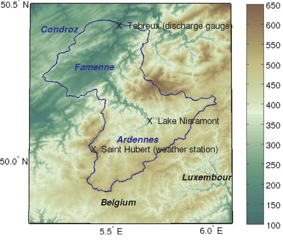
The Ourthe catchment is situated in the south-eastern part of Belgium and is partly 20

adjacent to North-West Luxembourg (Fig. 1). Near the city of Nisramont, the Ourthe Occidentale (Western branch) and the Ourthe Orientale (Eastern branch) join and form the river Ourthe. The catchment area south of this location is located in the Ardennes mountain range, which mainly consists of sandstone. From this point the river flows in a North-Westerly direction through a Middle-Devonian limestone area into the flat Fa-25

(5)

Con-HESSD

6, 7143–7178, 2009

climate change

Title Page

Tables Figures

◭ ◮

Back Close

Full Screen / Esc

droz region, which has Late-Devonian sandstone anticlines and Early-Carboniferous limestone synclines on top of the earlier mentioned shale. Since the higher Condroz region acts as a natural boundary, the Ourthe flows in a northerly direction, where several smaller tributaries, such as the Vesdre and the Ambl `eve, join the Ourthe river along its way towards Li `ege, where it eventually joins the river Meuse. This study only 5

addresses the catchment area upstream of Tabreux (Fig. 1). The Vesdre and Ambl `eve sub-catchments are, therefore, not taken into account. There are two main reasons to look at these systems separately: (1) the Ambl `eve and Vesdre are joining the Ourthe just before its outlet in the river Meuse and therefore do not affect much of the Ourthe catchment and (2) there is uncertainty in the discharge measurements just before the 10

confluence point of the Ourthe with the Meuse, because water levels depend on the setting of the weir at Angleur (Velner, 2000).

The Ourthe is a rain-fed river that is situated in a particularly hilly region and therefore has a fast discharge component in its hydrological system. This is especially the case in the upstream part of the catchment, where limited groundwater storage and steep 15

sandstone slopes are present. Altitudes vary roughly between 100 and 650 m a.s.l. With a length of 175 kilometers measured from the source of the Ourthe Occidentale it has an average hydraulic gradient of about 3 m km−1. The Ourthe catchment upstream of Tabreux, as defined in this study, has a surface area of about 1597 km2.

In the period between 1969 and 1998 the average yearly precipitation sum was 20

970 mm with a minimum of 680 mm and a maximum of 1230 mm measured at the weather station of St. Hubert. The average yearly evapotranspiration at St. Hubert was 590 mm and the average yearly discharge, as a result, 380 mm.

2.2 HBV model

The hydrological model used in this study to simulate the hydrological response of 25

(6)

suit-HESSD

6, 7143–7178, 2009

climate change

Title Page

Tables Figures

◭ ◮

Back Close

Full Screen / Esc

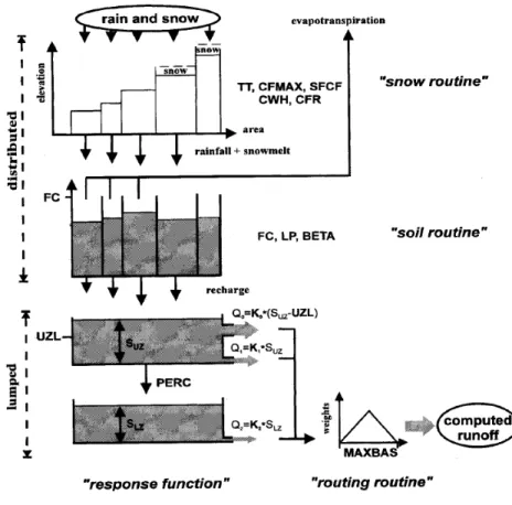
able for different purposes, such as simulation of long streamflow records, streamflow forecasting and hydrological proces research. It has been applied in many di_fferent catchments including the Rhine (te Linde et al., 2008; Hundecha and B ´ardossy, 2004) and the Meuse (Leander and Buishand, 2007; Booij, 2005). The model’s parameters are either measurable or significantly correlated to easily measurable catchment char-5

acteristics (Bergstr ¨om and Forsman, 1973). As can be seen schematically in Fig. 2, the HBV model describes the water balance using three storage reservoirs: a soil moisture zone, an upper zone storage (for sub-surface stormflow) and a lower zone storage. Including an algorithm for snow accumulation and melt (based on the degree-day method) and an algorithm accounting for lakes the general water balance equation 10

becomes the following:

P−E−Q₌ d

d t[SP+SM+U Z+LZ+l akes] (1)

whereP, E andQ refer to precipitation, evaporation and discharge, respectively. SP andSMstand for snow pack and soil moisture andU Z andLZ are related to the upper and lower groundwater zone. A subroutine for meteorological interpolation is available 15

to represent the spatial distribution of temperature and precipitation. The model re-quires precipitation, temperature and potential evapotranspiration as input (Seibert, 2005). For more details about the HBV model, see Bergstr ¨om and Forsman (1973) and Seibert (2005).

2.3 Datasets

20

As atmospheric forcing for the HBV model, daily observations of the weather station at St. Hubert (Fig. 1) are available, although all are spanning different periods: precipi-tation is available for 1968–2005 and temperature and potential evapotranspiration for 1968–1999. In addition, daily observed discharge at Tabreux is available for the period 1968–2005. Beside the observations, climate model output is available from the Max 25

(7)

HESSD

6, 7143–7178, 2009

climate change

Title Page

Tables Figures

◭ ◮

Back Close

Full Screen / Esc

(RCM) REMO (Jacob, 2001) is used to downscale data from either a Global Climate Model (GCM) or a re-analysis dataset, ERA15. For the ERA15 reanalysis dataset, as many global observations as possible have been collected for the period 1979–1993. In areas where the density of observation was sparse, satellite-based observations have been used. A data assimilation scheme and a numerical weather prediction model 5

propagated information about the state of the global atmosphere. This model output together with the observations and forcing fields were used as input for the reanalysis (Gibson et al., 1999). The ERA15 dataset is therefore a mixture of in-situ and satellite observations and modelled data. For this research, a version of the ERA15 dataset extended with operational analyses has been used. This dataset, spanning the period 10

1979–2003, downscaled using REMO to a horizontal resolution of 0.088◦(Jacob et al., 2008), is referred to as ERA hereafter.

Regional climate scenarios are used to force the HBV model to extract the effect of climate change. Three scenarios are available from the GCM ECHAM5/MPIOM, each spanning the period 2001–2100. The three climate scenarios are based on the A1B, A2 15

and B1 carbon-emission scenarios as they are defined by the IPCC (IPCC, 2000). The ECHAM5/MPIOM data, with a spatial resolution of about 400 km is downscaled in two steps by REMO (first to 0.44◦and then to 0.088◦; Jacob et al., 2008), similar to the ERA dataset. In addition, a reference dataset is available spanning the period 1951–2000, which also consists of downscaled ECHAM5/MPIOM data. Hereafter, the scenarios 20

and reference data from ECHAM5/MPIOM, downscaled with the REMO model, will be referred to as the ECHAM5 reference and scenario datasets. Although the ECHAM5 reference run resembles the current climate in a statistical sense, it cannot be used for model calibration because it does not represent the actual time series. The ERA dataset, on the other hand, contains observations and can, therefore, be used for 25

(8)

HESSD

6, 7143–7178, 2009

climate change

Title Page

Tables Figures

◭ ◮

Back Close

Full Screen / Esc

HBV model in order to extract the climate change signal.

3 Methodology

3.1 Bias correction

Because of the very low spatial resolution of a GCM, precipitation cannot be modelled explicitly but needs to be parameterized. This is one of the sources of structural model 5

errors in precipitation as modelled by GCMS (Lenderink et al., 2007). An extra error is added by the RCM in the downscaling process (Leander and Buishand, 2007). Before any hydrological application, the model biases need to be corrected for. However, there is only a long observational time series available for one weather station in the catch-ment, Saint Hubert (Fig. 1), which is situated at a relatively high altitude and close to 10

the boundary of the catchment. The first step is to compare di_fferent ways of correcting for the bias to assess which one results in the best representation of the observa-tions. To this end, an assessment of different bias correction methods is performed using the ERA dataset in order to find the best available method that can be applied to the ECHAM5 datasets. All atmospheric datasets contain three-hourly time series 15

for temperature, precipitation, atmospheric pressure, vapour pressure, shortwave and longwave incoming radiation and wind speed. However, corrections will only be applied to temperature and precipitation, since there are only observations available for these two parameters.

Several approaches to correct for model bias have been proposed (e.g., Leander 20

and Buishand, 2007; Shabalova et al., 2003; Hay et al., 2002). Leander and Buishand (2007) propose a power transformation, which corrects non-linearly for the coefficient of variation (CV) as well as the mean of the precipitation:

P∗₌a×Pb, (2)

(9)

HESSD

6, 7143–7178, 2009

climate change

Title Page

Tables Figures

◭ ◮

Back Close

Full Screen / Esc

a and b are parameters that define the correction. The parameters are iteratively estimated for each five-day period in a window including the 30 days before and after the five-day block over all years of the dataset, resulting in a 65-day window for each block. The value ofb is determined per block by matching the coefficient of variation (CV) of the corrected daily precipitation with the observed daily precipitation. The value 5

ofais then determined such that the mean of the transformed daily precipitation values matches the mean of the observed precipitation values. Thus, parameterb depends only on the CV and its determination is independent of parametera.

The bias correction of the temperature uses 73 blocks as well and involves shifting and scaling to adjust the mean and variance, respectively, according to:

10

T∗₌T_obs₊σ(Tobs) σ(T_cal)

T_uncor−T_obs₊T_obs−T_cal, (3)

where T_uncor and T∗ represent the uncorrected daily temperature and the corrected daily temperature, respectively. T_obs andσ(T_obs) are the mean and standard deviation of the observed daily temperature for the considered five-day period. Similarly, T_cal andσ(T_cal) are the mean and standard deviation of the uncorrected temperature for the 15

considered five-day period. The same bias correction methodology was also applied to the Rhine basin by Hurkmans et al. (2009b), and was investigated in detail by Terink et al. (2009). They show that after the correction not only the estimation of average precipitation was improved, but also for example that of extreme values, 10-day sums and the first order autocorrelation.

20

Because the spatial resolution of the climate model data is 0.088◦(about 10 km), and the observations are only available for one location, different approaches are possible to perform the bias correction. Parameters a and b can, for example, be calculated based on the grid cell corresponding to Saint Hubert, or based on the spatial average (assuming that the observation is representative for the entire catchment). Four ap-25

(10)

HESSD

6, 7143–7178, 2009

climate change

Title Page

Tables Figures

◭ ◮

Back Close

Full Screen / Esc

observation. The second method averages the uncorrected data of all the grid cells into one spatially averaged time series and compares it with the Saint Hubert observation. The set of calculated parameters is then applied to all the grid cells. The third method calculates one set of correction parameters by comparing the uncorrected data of the grid cell corresponding to Saint Hubert (denoted as cell 90) and applies this set to all 5

the grid cells. The fourth and last method is similar to the third method, but employs a neighbouring grid cell (denoted as cell 80), that better represents the observations at Saint Hubert in terms of monthly precipitation sums than cell 90.

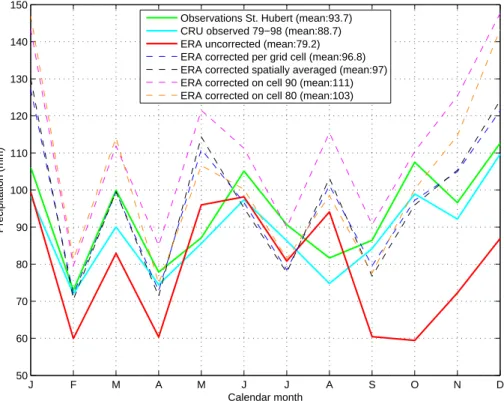
The correction parameters for precipitation are based on the time period 1979–2003, whereas those for temperature are based on the time period 1979–1996. Figure 3 10

shows the temporal distribution of mean monthly precipitation sums averaged over all the grid cells. A dataset of the Climate Research Unit (CRU) that contains observed monthly averages is plotted as well in order to compare to what extent the Saint Hubert weather station approximates the spatial average. This dataset is also used to repre-sent the average precipitation sums for the Ourthe catchment and shows a very similar 15

climatology compared to the Saint Hubert observation. Therefore, it can be argued that the single observation of Saint Hubert is close to representing the entire catchment at the monthly time scale. In terms of mean monthly precipitation sums, the observations are closest to the correction per grid cell and the spatially averaged correction method. Figure 4 shows the temporal distribution of mean monthly temperature averaged over 20

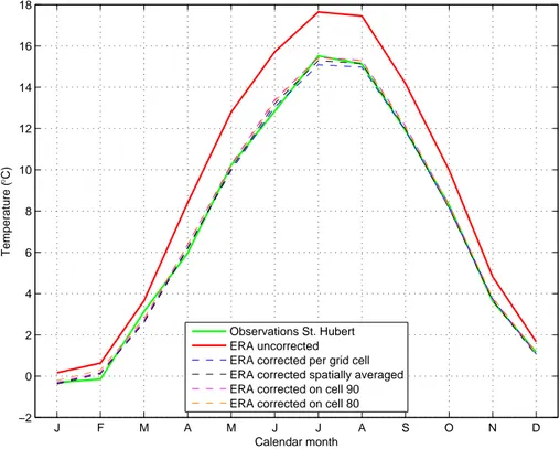
all the grid cells. It can be seen directly that the bias corrections for temperature are very solid for practically every method. Furthermore, the error of the uncorrected ERA dataset with respect to the observations appears to be larger in summertime than in wintertime.

The overall mean of the uncorrected ERA dataset is lower than that of the observa-25

(11)

maxi-HESSD

6, 7143–7178, 2009

climate change

Title Page

Tables Figures

◭ ◮

Back Close

Full Screen / Esc

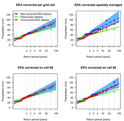
mum daily precipitation sums of cell 90 versus their return period over 25 years and fits a Gumbel distribution through the data points. Each subplot consists of three datasets of which the observations, the green line, and the uncorrected dataset, the red line, are shown in every plot to put the bias-corrected dataset, that is plotted in blue, in perspective.

5

Furthermore, the four subplots each contain a corresponding 95%-confidence-interval of the bias-corrected dataset that is produced using the profiling log-likelihood method (Smith, 1985). This is a method to take into account the uncertainty in the fitted Gumbel distribution without making additional assumptions. At every quantile of the dataset of annual discharge maxima, corresponding to the return period in Fig. 5 10

(q_(0.02),q_(0.03),q_(0.05),q_(0.10),q_(0.25),q_(0.50),q_(1.00)), the GEV or Gumbel distribution is reparameterized such that the specific quantile becomes one of the parameters (Coles, 2001). At each quantile (or return period), the 95%-confidence-interval is then es-timated from the resulting likelihood function using an iterative method (Venzon and Moolgavkar, 1988).

15

Figure 5 also shows that the Gumbel fit of the uncorrected dataset is on a higher level than the fits corresponding to the observation dataset. It indicates that the method that corrects per grid cell and the method that corrects on cell 90 both show a fit that is situated between the observed and uncorrected dataset, while the other methods both have a Gumbel fit that is situated above those of the observation dataset as well as the 20

uncorrected dataset.

Based on the performance of the different methods, one should be selected to force the hydrological model. The analysis above shows that there are big differences be-tween the observation dataset and the uncorrected dataset with respect to precipitation sums and climatologies. The bias correction per grid cell and on spatially averaged 25

(12)

HESSD

6, 7143–7178, 2009

climate change

Title Page

Tables Figures

◭ ◮

Back Close

Full Screen / Esc

shown). In contrast to the correction of precipitation, the correction of the temperature time series is successful for all the four methods and results in bias corrected datasets that show the same magnitude and timing as the observed temperature time series.

The bias correction based on a spatially averaged precipitation time series produces a dataset that has a mean which is closest to the observation dataset. The extreme 5

value analysis of the yearly precipitation maxima of cell 90, where Saint Hubert is lo-cated, shows not much deviation between the datasets. The largest difference between the datasets at a return period of 100 years based on a Gumbel distribution is about 15 mm. The di_fference between the uncorrected ERA dataset and the observation dataset is small and their trend lines cross each other at a return period of approxi-10

mately two years. It is likely that the Gumbel plot representing the Ourthe catchment the best on average should be situated between the green and red trend lines. Figure 3 shows that the mean of the uncorrected dataset is significantly less than they are in the observation dataset. Thus, when putting these graphs next to Fig. 5 it can be stated that the uncorrected ERA dataset underestimates the total volume of precipitation, but 15

it slightly overestimates the extremes for return periods larger than 2 years with respect to the observations of Saint Hubert. Based on the interpretations above the bias cor-rection method that corrects spatially averaged data is chosen as the best method to correct the ERA dataset.

Throughout the analyses the bias correction method that corrects per grid cell and 20

the method that corrects spatially averaged times series have shown reasonable re-sults. The strongest argument to choose the latter is based on the preservation of the spatial distribution of precipitation and the fact that less weight is put on the overes-timation of extreme precipitation. A strong emphasis should be put on the fact that the method that corrects on spatially averaged time series is the best method of the 25

(13)

HESSD

6, 7143–7178, 2009

climate change

Title Page

Tables Figures

◭ ◮

Back Close

Full Screen / Esc

Before forcing the HBV model, the ECHAM5 reference and scenario datasets have to be bias-corrected using the observations. The reference period is corrected for the period 1961–2000, where the parameter values for temperature are based on the the period 1968–1996, and those for precipitation are based on the period 1968–2000. The same parameter values are then applied to correct the three ECHAM5 scenario 5

datasets for the period 2001–2100, assuming that the bias is stationary and will not change under future conditions. This is a common assumption to make as there is often no information about the stationarity of the bias (e.g., Hurkmans et al., 2009b; van Pelt et al., 2009; Leander and Buishand, 2007). However, it may not be completely valid as the bias tends to increase with increasing temperatures (Christensen et al., 10

2008).

3.2 Model calibration

The HBV model requires precipitation, temperature and potential evaporation as input. As already mentioned, the observations are available for the time period 1968–1996 and are suitable to calibrate the model with. Before the calibration is started, the catch-15

ment is divided into five elevation zones, each with its own areal fraction. The elevation zones are used to lapse precipitation and temperature with elevation: precipitation is assumed to increase by 10% with every increase of 100 m and temperature is assumed to decrease with 0.61◦C per 100 m increase in elevation. The fraction of lakes is set to 0.0003, due to the presence of the Lake of Nisramont which has a surface area of 20

0.47 km2, and the elevation of the precipitation and temperature measurements is fixed at 553 m, because this corresponds with the altitude of Saint Hubert.

Fifteen parameters are included in the calibration, see Seibert (2000) for details and parameter ranges. The calibration is carried out using the GAP optimization tool (Genetic Algorithm andPowell), that refers to a genetic algorithm to approximate the 25

(14)

gen-HESSD

6, 7143–7178, 2009

climate change

Title Page

Tables Figures

◭ ◮

Back Close

Full Screen / Esc

erated parameter sets that are located within the given ranges. These sets are being evaluated by running the model and thus the goodness of fit of each set is determined by the value of the employed objective function. Parameter sets with a good value are given a higher probability to generate new sets than those sets that gave poorer results (Seibert, 2000). The multi-criteria objective function used in this research is a combi-5

nation of the well-known Nash-Sutcli_ffe modelling e_fficiency R_e_ff (Nash and Sutcli_ffe, 1970), and the absolute value of the volume error,|V E|, in mm per year.

Calibration is carried out for the time period 1969–1988, i.e. 20 years, whereas 1968 is used to initialize the system. For validation, the time period 1989–1996 will be used. The calibration period is substantially larger than the validation period, because after 10

the model has been calibrated and validated it has to be able to run large scenario datasets of 100 years. It is expected that calibration on a long time period is beneficial in order to reach this ability. In this calibration and forecasting process the assumption is made that calibrated parameters stay constant over time. The results of calibration and validation runs showed the best performance for the validation period with aR_e_ff of 15

0.89, a|V E| of 8 mm and a correlation coefficient of 0.90, while the calibration period showed aR_e_ffof 0.84, a|V E|of 34 mm and a correlation coefficient of 0.86.

3.3 Calculation of potential evaporation

Potential evaporation is not included in the forcing dataset, therefore it needs to be cal-culated based on the available forcing parameters to make the reference and scenario 20

datasets suitable as HBV input. For this purpose the simplified Makkink equation is used (Makkink, 1957):

Lv×E T_ref₌0.65× s s₊γ×K

↓ ₍₄₎

(15)

HESSD

6, 7143–7178, 2009

climate change

Title Page

Tables Figures

◭ ◮

Back Close

Full Screen / Esc

is the parameter that has to be calculated in order to obtain the potential evapotran-spiration;s is the slope of the saturated water vapour pressure curve in kPa K−1;K↓is the incoming solar radiation in W m−2;γ the psychrometric constant in kPa K−1. Once the reference evapotranspiration is calculated the potential evapotranspiration,E T_p, is calculated with use of the crop factor,k_c:

5

E T_p₌k_c×E T_ref (5)

The crop factor is based on the vegetation cover of the Ourthe catchment, which is provided by the PELCOM database (M ¨ucher et al., 2000). The Ourthe is divided into six land cover types, each with a specific crop factor (given within parentheses; Makkink, 1957): coniferous (1.30), deciduous (1.04) and mixed forest (1.17), grass (1.0), arable 10

rain-fed crops (1.0) and urban area (1.0). Multiplying the crop factor of each land cover type with the corresponding surface fraction results in the average crop factor of 1.06. With this general correction reasonable evapotranspiration values are created using the incoming solar radiation, air temperature and atmospheric pressure of the bias-corrected ECHAM5 dataset.

15

4 Results and discussion

The calibrated HBV model is then used to simulate discharges at Tabreux for the ECHAM5 reference period and the three ECHAM5 climate scenarios. Time periods of 39 years are selected in order to enable a fair comparison between the reference period and the climate scenarios. The reference period uses one year as warming-up 20

period for initialization and thus simulates the period 1962–2000. The climate scenario datasets contain forcing input for 100 years, while the maximum number of timesteps accepted by HBV Light is 20 000. Therefore two consecutive model runs are needed to capture a 100-year scenario. In the time series that are now created (2002–2100) two periods are isolated, so that clear climate signals can be distinguished: the be-25

(16)

HESSD

6, 7143–7178, 2009

climate change

Title Page

Tables Figures

◭ ◮

Back Close

Full Screen / Esc

The ECHAM5 reference and scenario forcing data are averaged over the catchment and, therefore, the model parameter indicating the elevation of the temperature and precipitation measurement needs to be set at 250.64 m, which is the average elevation of the Ourthe catchment.

4.0.1 Mean outflow

5

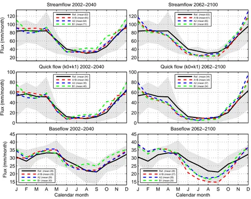
First, the average monthly values of the individual discharge components are investi-gated. For the beginning and end of the 21st century, Fig. 6 shows the quick upper zone outflux, created by the sum of Q₀ and Q₁ (Fig. 2), the slower outflux from the lower zone,Q₂, and the total streamflow, i.e. the sum of all fluxes. In the first part of the century the scenarios have a monthly climatology that is similar to the reference, 10

but the average total discharge is somewhat higher. Especially the B1 scenario has a high monthly mean of 71 mm and produces the highest discharges in the period from August to January. This increase is strongest in the months January, October and De-cember, when it is ranging between 20% and 54%. The higher discharge of the B1 scenario can be explained due to the increased precipitation for this scenario. In the 15

second part of the century, all the scenario curves have evolved in a more pronounced way. All scenarios indicate less discharge for the months April until September, while in the months December and January discharge is 27% to 38% higher compared to the reference. The overall mean of the scenario discharge has further increased for the A2 scenario, while the discharges for the A1B and B1 scenarios decrease with respect to 20

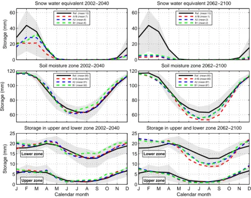
the beginning of the century and the reference discharge. The total streamflow graphs also show the almost constant discharge of the reference dataset for the months De-cember until April, which can be explained by the buffering effect due to the presence of snow in the catchment. The volume of the snowpack is shown in the upper two plots of Fig. 7, which show very clearly that the storage of snow is diminishing with time. 25

(17)

HESSD

6, 7143–7178, 2009

climate change

Title Page

Tables Figures

◭ ◮

Back Close

Full Screen / Esc

and results in a discharge climatology that shows hardly any buffering effect by the snowpack.

The quick flow and baseflow plots in Fig. 6 show similar trends compared the total streamflow of the Ourthe. In winter, the quick flow component is almost twice as large as the baseflow component, while in summer the baseflow is larger than the quick flow 5

component. This e_ffect occurs mainly due to the large variation in the mean monthly quick flow, which can differ 70 mm on a monthly basis throughout the year. The gray shaded areas in Fig. 6 indicate the range between the 25th and 75th percentile of the reference dataset and show the variation of mean discharges in the 39-year reference period. From these ranges, it can be concluded that the mean monthly discharge of 10

total streamflow during winter has a larger variation than the mean monthly discharge during summer.

4.0.2 Mean storages

The changes in streamflow are in the first place produced by a change in forcing. How-ever, this change is also a_ffecting the storage in the catchment reservoirs. Assessing 15

the di_fferent reservoirs gives a further insight why changes in the streamflow occur. On average, the reference period is characterized by snow in the months December until April and a snow storage peak in February of about 44 mm (Fig. 7). All the climate scenarios show a decrease in snow storage in the beginning of the century that ex-tends towards the end of the century. The mean monthly storages in the soil moisture 20

zone are also plotted in Fig. 7 and show that in the winter months December, January and February the soil moisture zone is nearly saturated until the field capacity value of 119.9 mm. At the end of the 21th century, the mean storage in the soil moisture zone is clearly less than during the reference period, which is mainly due to the decreased water storage in the summer months. This decrease is most pronounced for the A1B 25

(18)

HESSD

6, 7143–7178, 2009

climate change

Title Page

Tables Figures

◭ ◮

Back Close

Full Screen / Esc

be explained by the fact that the outflow of the lower reservoir is smaller due to its re-cession coe_fficient,K₂, that is three to five times smaller than the recession coe_fficients for the upper zone outflow. Structural changes in storage become more distinctive to-wards the end of the century, especially in the lower zone storage. During the months May until October, less water is stored in this reservoir and the opposite is true for the 5

months November until April. Thus, the seasonal e_ffect in storage becomes stronger for all scenarios.

4.0.3 Streamflow droughts

In this study, a drought occurs when the discharge drops below a certain threshold. This threshold is arbitrary and is in this case defined as the 75th percentile of the 10

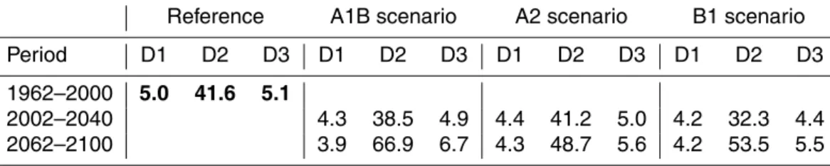
reference period, i.e., the discharge that is exceeded for 75% of the time. Thus, the lower 25% of the daily discharges are considered as belonging to a drought (Fleig et al., 2006; Hurkmans et al., 2009a,b). For the Ourthe this comes down to a threshold discharge of 14.05 m3s−1. In Table 1 drought statistics are shown for the reference period as well as for the several scenarios for the two time periods that have been 15

considered.

The results presented in Table 1 differ strongly throughout the 21st century. In the beginning of the century, all three indicators decrease for all scenarios. The B1 sce-nario in particular is characterized by an average annual maximum duration of about 32 days, which represents a decrease of 25% with respect to this statistic during the ref-20

erence period. At the end of the century, the average number of events has decreased even further, but the average of annual maximum durations shows large increases with respect to the beginning of the century, especially for the A1B and B1 scenarios. The difference of the A1B and B1 scenarios with respect to the reference period is about 25 and 12 days, respectively. Remarkable is also that all scenarios show a significantly 25

(19)

HESSD

6, 7143–7178, 2009

climate change

Title Page

Tables Figures

◭ ◮

Back Close

Full Screen / Esc

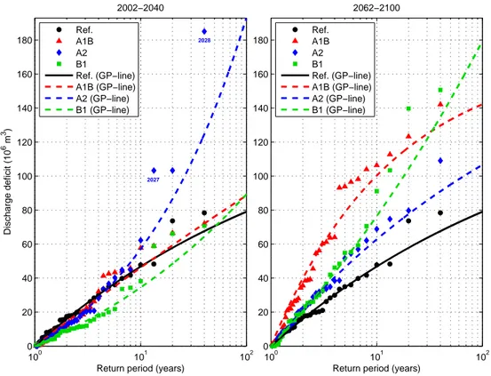
Streamflow droughts can also be analyzed by plotting the distribution of the annual maximum cumulative deficit volumes as a function of their return period (Hurkmans et al., 2009b), as can be seen in Fig. 8. A Generalized Pareto (GP) distribution is fitted through the data points. For the beginning of the century, not much difference can be seen between the A1B scenario and the reference period. The B1 scenario 5

clearly indicates, through its data points as well as through its fitted distribution, that smaller discharge deficit volumes are expected for the same return period with respect to the reference period, while the A2 scenario follows the same curve as the reference period until a return period of about six years. For higher return periods, the data points and the fitted distribution are situated above the data points and distribution of 10

the reference. However, it should be stressed that mainly the three highest discharge deficits of the A2 scenario play a role in producing the convex shape of the fitted line. Not too much emphasis should be put on this peculiar shape, because the number of available data points for high return periods is small. At the end of the century, all the data points and fitted distributions of the scenarios indicate significantly larger annual 15

maximum discharge deficit volumes than the reference for the same return periods. The di_fference with respect to the reference becomes larger with increasing return periods for the A2 and B1 scenarios. This increase is larger for the B1 scenario than for the A2 scenario. Still, the A1B scenario shows already large differences at low return periods. The increased discharge deficit volumes of the A1B scenario was expected, 20

since Table 1 also showed a considerable increase in annual maximum duration and intensity.

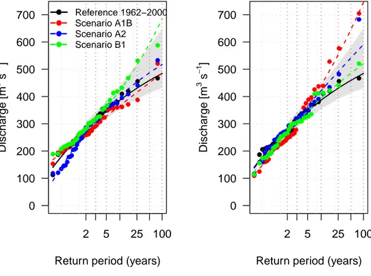
4.1 Peak discharges

For water management purposes, an analysis of the maximum daily discharge is also of importance. In Fig. 9, two graphs show the extreme peak discharges of the scenar-25

(20)

HESSD

6, 7143–7178, 2009

climate change

Title Page

Tables Figures

◭ ◮

Back Close

Full Screen / Esc

are situated between a return period of 5 and 15 years and have nearly the same dis-charge level. The A2 scenario has lower peak disdis-charges at low return periods, but follows the reference period quite closely for return periods above two years. In con-trast, the B1 scenario has higher peak discharges for return periods above five years with respect to the reference. Towards the end of the century, the A1B scenario shows 5

lower peak discharges than the reference for return periods lower than 3 years, but higher peak discharges than the reference for higher return periods. Furthermore, five of the six highest peak discharges are situated above the 95%-confidence interval of the reference, meaning that under the A1B scenario it is even more likely that higher peak discharges occur.

10

5 Summary and conclusions

By means of high-resolution regional climate scenarios and a well-known hydrological model, we have obtained projections of the hydrological behaviour of the Ourthe catch-ment during the 21st century. In addition, an important step in this process, the bias correction of the climate model output has been investigated extensively. Although 15

ERA15 is often used to represent data (e.g., Kotlarski et al., 2005; Hurkmans et al., 2008), for precipitation large di_fferences with respect to the observations appear when considering a relatively small catchment such as the Ourthe. Because the bias merely corrects for mean and variability of the precipitation, after bias correction still consider-able di_fferences exist between modelled and observed precipitation time series. This 20

should be kept in mind when interpreting our results. Four di_fferent bias correction methods have been assessed by looking at the mean monthly values and the spatial distribution for temperature and precipitation, as well as extreme precipitation events. It can be concluded that determination of the bias correction parameters of a spatially averaged dataset after which the same parameters are applied to each grid cell, yields 25

(21)

HESSD

6, 7143–7178, 2009

climate change

Title Page

Tables Figures

◭ ◮

Back Close

Full Screen / Esc

By comparing the beginning, 2002–2040, and the end, 2062–2100, of the 21st cen-tury with the reference period, 1962–2000, changes in various hydrological variables are investigated. For many variables, the change in the beginning is not so pronounced as it is towards the end of the century. This is true for practically every scenario. In general, the discharge of the Ourthe is characterized by a growing contrast between 5

seasons, meaning that the winters become wetter and the summers become drier. This holds for all three scenarios that were investigated. The overall annual streamflow increases during the entire century according to all scenarios. Only the A1B scenario projects a small decrease towards the end of the century. All scenarios, A1B being the most extreme, project a decrease in baseflow in the summer months, associated with 10

declining soil moisture and groundwater storages in the summer. Especially in the A2 and A1B scenarios, snow storage is declining throughout the century and practically disappearing towards the end of the century. Also in the B1 scenario it is decreasing, but not as dramatic as in the other two scenarios due to the relatively small temper-ature increase in the B1 scenario. Streamflow droughts typically decrease during the 15

beginning of the century due to the increase of precipitation and discharge. In con-trast, more extreme streamflow droughts are projected to occur towards the end of the century. This holds for all scenarios, again the A1B scenario being the most extreme. Peak flows are not projected to change dramatically or even decrease slightly, except for the B1 scenario in the beginning of the century, where the extreme peak flows are 20

somewhat higher than in the reference situation. The same holds for the A1B scenario at the end of the century.

A drawback of the employed bias correction is the availability of data at only one lo-cation. If available, future research should therefore incorporate multiple observations points in order to get a better representation of average precipitation and temperature 25

(22)

HESSD

6, 7143–7178, 2009

climate change

Title Page

Tables Figures

◭ ◮

Back Close

Full Screen / Esc

forcing input. Experiments where GCMs have been compared (e.g., Covey et al., 2003; Reichler and Kim, 2008) indicated a large range even in simulations of the current cli-mate, let alone for a future climate. See Hurkmans et al. (2009b) for a more extensive discussion regarding this problem. Using multiple or other models would take into ac-count such a range. Similar comparisons, however, showed that the GCM that was 5

used in this study very well simulates the current climate and is relatively close to the multi-model mean in ensemble projections (IPCC, 2007).

Acknowledgements. This research was financially supported by the European Commission

through the FP6 Integrated Project NeWater and the BSIK ACER project of the Dutch Climate Changes Spatial Planning Programme. The authors would like to thank Roel Velner and the

10

KMI for making available observed data for the Ourthe catchment. Daniela Jacob from the Max Planck Institut f ¨ur Meteorologie in Hamburg, Germany is kindly acknowledged for making available the downscaled climate scenarios.

References

Arpe, K., Hagemann, S., Jacob, D., and Roeckner, E.: The realism of the ECHAM5 models to

15

simulate the hydrological cycle in the Arctic and North European area, Nordic Hydrology, 36, 349–367, 2005. 7145

Bergstr ¨om, S. and Forsman, A.: Development of a conceptual deterministic rainfall-runoff

model, Nord. Hydrol., 4, 147–170, 1973. 7146, 7147, 7148

Berne, A., ten Heggeler, M., Uijlenhoet, R., Delobbe, L., Dierickx, P., and de Wit, M.: A

prelimi-20

nary investigation of radar rainfall estimation in the Ardennes region and a first hydrological application for the Ourthe catchment, Nat. Hazards Earth Syst. Sci., 5, 267–274, 2005, http://www.nat-hazards-earth-syst-sci.net/5/267/2005/. 7146

Booij, M. J.: Impact of Climate Change on River Flooding Assessed with Different Spatial Model Resolutions, J. Hydrol., 303, 176–198, doi:10.1016/J.Hydrol.2004.07.013, 2005. 7145, 7148

25

Chbab, E. H.: How extreme were the 1995 flood waves on the rivers Rhine and Meuse?, Phys. Chem. Earth, 20, 455–458, 1995. 7145

(23)

HESSD

6, 7143–7178, 2009

climate change

Title Page

Tables Figures

◭ ◮

Back Close

Full Screen / Esc

Interactive Discussion correction of regional climate change projections of temperature and precipitation, Geophys.

Res. Lett., 35, L20709, doi:10.1029/2008GL035694, 2008. 7155

Coles, S.: An introduction to statistical modeling of extreme values, Springer series in statistics, Springer Verlag, 2001. 7153

Covey, C., AchutaRao, K. M., Cubasch, U., Jones, P., Lambert, S. J., Mann, M. E., Philips, T. J.,

5

and Taylor, K. E.: An overview of results from the Coupled Model Intercomparison Project, Global Planet. Change, 37, 103–133, doi:10.1016/S092108181(02)00193-5, 2003. 7164 de Wit, M., Warmerdam, P., Torfs, P., Uijlenhoet, R., E.Roulin, Cheymol, A., van Deursen, W.,

van Walsum, P., Ververs, M., Kwadijk, J., and Buiteveld, H.: Effect of climate change on the hydrology of the river Meuse, Tech. Rep. 410 200 090, Dutch National Research Programme

10

on Global Air Pollution and Climate Change, 2001. 7145

de Wit, M. J. M., van den Hurk, B., Warmerdam, P. M. M., Torfs, P. J. J. F., Roulin, E., and van Deursen, W. P. A.: Impact of climate change on low-flows in the river Meuse, Clim. Change, 82, 351–372, doi:10.1007/S10584-006-9195-2, 2007. 7144, 7145

Fleig, A. K., Tallaksen, L. M., Hisdal, H., and Demuth, S.: A global evaluation of streamflow

15

drought characteristics, Hydrol. Earth Syst. Sci., 10, 535–552, 2006, http://www.hydrol-earth-syst-sci.net/10/535/2006/. 7160

Gibson, J., Kallberg, P., Uppala, S., Hernandez, A., Nomura, A., and Serrano, E.: ECMWF Re-Analysis Project Report Series: 1. ERA-15 Description (version 2), Tech. rep., ECMWF, 1999. 7149

20

Hay, L. E., Clark, M. P., Wilby, R. L., Jr., W. J. G., Leavesly, G. H., Pan, Z., Arritt, R. W., and Takle, E. S.: Use of regional climate model output for hydrologic simulations, J. Hydromete-orol., 3, 571–590, 2002. 7150

Hazenberg, P., Weerts, A., Reggiani, P., Delobbe, L., Leijnse, H., and Uijlenhoet, R.: Weather radar estimation of large scale stratiform winter precipitation in a hilly environment and its

25

implications for rainfall runoffmodeling, Water Resour. Res., in review, 2009. 7146

Hundecha, Y. and B ´ardossy, A.: Modeling of the effect of land use changes on the runoff gen-eration of a river basin through parameter regionalization of a watershed model, J. Hydrol., 292, 281–295, doi:10.1016/j.jhydrol.2004.01.002, 2004. 7148

Hurkmans, R. T. W. L., de Moel, H., Aerts, J. C. J. H., and Troch, P. A.: Water balance versus

30

land surface model in the simulation of Rhine river discharges, Water Resour. Res., 44, W01418, doi:10.1029/2007WR006168, 2008. 7162

(24)

HESSD

6, 7143–7178, 2009

climate change

Title Page

Tables Figures

◭ ◮

Back Close

Full Screen / Esc

Interactive Discussion Effects of land use changes on streamflow generation in the Rhine basin, Water Resour.

Res., 45, W06405, doi:10.1029/2008WR007574, 2009a. 7160

Hurkmans, R. T. W. L., Terink, W., Uijlenhoet, R., Torfs, P. J. J. F., Jacob, D., and Troch, P. A.: Changes in streamflow dynamics in the Rhine basin under three high-resolution climate scenarios, J. Climate, in press, doi:10.1175/2009JCLI3066.1, 2009b. 7145, 7151, 7155,

5

7160, 7161, 7164

IPCC: Special report on emissions scenarios - a special report of working group III of the In-tergovernmental Panel on Climate Change, http://www.grida.no/climate/ipcc/emission/index. htm, 2000. 7149

IPCC: Fourth assessment report: Climate change 2007: Climate change impacts, adaptation

10

and vulnerability. Summary for policy makers., 2007. 7145, 7164

Jacob, D.: A note to the simulation of the annual and inter-annual variability of the water budget over the Baltic Sea drainage basin, Meteorol. Atmos. Phys., 77, 61–73, 2001. 7145, 7149 Jacob, D., G ¨ottel, H., Kotlarski, S., Lorenz, P., and Sieck, K.: Klimaauswirkungen und

An-passung in Deutschland – Phase 1: Erstellung regionaler Klimaszenarien f ¨ur Deutschland,

15

Forschungsbericht 204 41 138 UBA-FB 000969, Umweltbundesamt, Dessau, Germany, 2008. 7149

Kotlarski, S., Block, A., B ¨ohm, U., Jacob, D., Keuler, K., Knoche, R., Rechid, D., and Walter, A.: Regional climate model simulations as input for hydrological applications: evaluation of uncertainties, Adv. Geosci., 5, 119–125, 2005,

20

http://www.adv-geosci.net/5/119/2005/. 7162

Kwadijk, J. and Rotmans, J.: The impact of climate change on the river Rhine: a scenario study, Clim. Change, 30, 397–425, 1995. 7145

Leander, R. and Buishand, T. A.: Resamping of regional climate model output for the simulation of extreme river flows, J. Hydrol., 332, 487–496, doi:10.1016/j.jhydrol.2006.08.006, 2007.

25

7148, 7150, 7155

Leander, R. and Buishand, T. A.: A weather generator based on a two-stage resampling algo-rithm, J. Hydrol., 374, 185–195, doi:10.1016/j.jhydrol.2009.06.010, 2009. 7146

Lenderink, G., Buishand, T. A., and van Deursen, W. P.: Estimates of future discharges of the river Rhine using two scenario methodologies: direct versus delta appraoch, Hydrol. Earth

30

Syst. Sci., 11, 1145–1159, 2007,

http://www.hydrol-earth-syst-sci.net/11/1145/2007/. 7145, 7146, 7150

(25)

circula-HESSD

6, 7143–7178, 2009

climate change

Title Page

Tables Figures

◭ ◮

Back Close

Full Screen / Esc

Interactive Discussion tion: a two-way nesting climate simulation, Geophys. Res. Lett., 32, L18706, doi:10.1029/

2005GL023351, 2005. 7145

Makkink, G.: Testing the Penman formula by means of lysimeters, International J. Water Eng., 11, 277–288, 1957. 7156, 7157

M ¨ucher, S., Steinnocher, K., Champeaux, J.-L., Griguolo, S., Wester, K., Heunks, C., and van

5

Katwijk, V.: Establishment of a 1-km Pan-European Land Cover database for environmental monitoring, in: Proceedings of the Geoinformation for All XIXth Congress of the International Society for Photogrammetry and Remote Sensing (ISPRS), edited by: Beek, K. J. and Mole-naar, M., vol. 33 of Int. Arch. Photogramm. Remote Sens., 702–709, GITC, Amsterdam., 2000. 7157

10

Nash, J. E. and Sutcliffe, I. V.: River flow forecasting through conceptual models. Part I – A discussion of principles, J. Hydrol., 10, 282–290, 1970. 7156

Press, W., Flannery, B., Teukolsky, S., and Vetterling, W.: Numerical recipes in FORTRAN: The art of scientific computing, Cambridge University Press, Cambridge, Great Britain, 2nd edition edn., 1992. 7155

15

Reichler, T. and Kim, J.: How well do coupled models simulate today’s climate?, Bull. Amer. Meteor. Soc., 89, 303–311, doi:10.1175/BAMS-89-3-303, 2008. 7164

Seibert, J.: Multi-criteria calibration of a conceptual runoff model using a genetic algorithm, Hydrol. Earth Syst. Sci., 4, 215–224, 2000,

http://www.hydrol-earth-syst-sci.net/4/215/2000/. 7155, 7156, 7171

20

Seibert, J.: HBV light version 2, User’s manual, Dept. of Physical Geography and Quaternary Geology, Stockholm University, 2005. 7146, 7147, 7148

Shabalova, M. V., van Deursen, W. P. A., and Buishand, T. A.: Assessing future discharge of the river Rhine using regional climate model integrations and a hydrological model, Climate Res., 23, 233–246, 2003. 7145, 7150

25

Smith, R. L.: Maximum likelihood estimation in a class of nonregular cases, Biometrika, 72, 67–90, 1985. 7153

te Linde, A. H., Aerts, J. C. J. H., Hurkmans, R. T. W. L., and Eberle, M.: Comparing model performance of two rainfall-runoff models in the Rhine basin using different atmospheric forcing data sets, Hydrol. Earth Syst. Sci., 12, 943–957, 2008,

30

http://www.hydrol-earth-syst-sci.net/12/943/2008/. 7148

(26)

HESSD

6, 7143–7178, 2009

climate change

Title Page

Tables Figures

◭ ◮

Back Close

Full Screen / Esc

Interactive Discussion Hydrol. Earth Syst. Sci. Discuss., 6, 5377–5413, 2009,

http://www.hydrol-earth-syst-sci-discuss.net/6/5377/2009/. 7151

Trenberth, K. E., Dai, A., Rasmussen, R. M., and Parsons, D. B.: The changing character of precipitation, Bull. Amer. Meteor. Soc., 84, 1205–1217, doi:10.1175/BAMS-84-9-1205, 2003. 7145

5

van Pelt, S. C., Kabat, P., ter Maat, H. W., van den Hurk, B. J. J. M., and Weerts, A. H.: Discharge simulations performed with a hydrological model using bias corrected regional climate model input, Hydrol. Earth Syst. Sci. Discuss., 6, 4589–4618, 2009,

http://www.hydrol-earth-syst-sci-discuss.net/6/4589/2009/. 7145, 7155

Velner, R.: Neerslag-afvoer modellering van het stroomgebeid van de Ourthe met het HBV

10

model: een studie ten behoeve van verlenging van de zichttijd van hoogwatervoorspelling op de Maas, Master’s thesis, Wageningen University, 2000. 7147

(27)

HESSD

6, 7143–7178, 2009

climate change

Title Page

Tables Figures

◭ ◮

Back Close

Full Screen / Esc

Table 1.Statistics of drought events for the reference period and the climate scenarios for the

period 2002–2040 and 2062–2100. A drought event is calculated with respect to a specific threshold discharge. The statistical parameters are indicated with D1, D2 and D3, where D1 is the average number of events per year, D2 is the average of the yearly maximum durations of a drought in days, and D3 is the average of yearly maximum intensities, where the intensity is defined as the deficit volume divided by duration, in m3s−1.

Reference A1B scenario A2 scenario B1 scenario

Period D1 D2 D3 D1 D2 D3 D1 D2 D3 D1 D2 D3

1962–2000 5.0 41.6 5.1

(28)

HESSD

6, 7143–7178, 2009

climate change

Title Page

Tables Figures

◭ ◮

Back Close

Full Screen / Esc

Fig. 1. Digital elevation model of the Ourthe catchment. Also shown are the discharge

(29)

HESSD

6, 7143–7178, 2009

climate change

Title Page

Tables Figures

◭ ◮

Back Close

Full Screen / Esc

(30)

HESSD

6, 7143–7178, 2009

climate change

Title Page

Tables Figures

◭ ◮

Back Close

Full Screen / Esc

J F M A M J J A S O N D

50 60 70 80 90 100 110 120 130 140 150

Calendar month

Precipitation (mm)

Observations St. Hubert (mean:93.7) CRU observed 79−98 (mean:88.7) ERA uncorrected (mean:79.2) ERA corrected per grid cell (mean:96.8) ERA corrected spatially averaged (mean:97) ERA corrected on cell 90 (mean:111) ERA corrected on cell 80 (mean:103)

Fig. 3.Mean monthly precipitation sums of the observations and (un)corrected datasets for the

(31)

HESSD

6, 7143–7178, 2009

climate change

Title Page

Tables Figures

◭ ◮

Back Close

Full Screen / Esc

J F M A M J J A S O N D

−2 0 2 4 6 8 10 12 14 16 18

Calendar month

Temperature (

°

C)

Observations St. Hubert ERA uncorrected ERA corrected per grid cell ERA corrected spatially averaged ERA corrected on cell 90 ERA corrected on cell 80

Fig. 4.Mean monthly temperature of the observations and (un)corrected datasets for the period

(32)

HESSD

6, 7143–7178, 2009

climate change

Title Page

Tables Figures

◭ ◮

Back Close

Full Screen / Esc

Return period (years)

Precipitation (mm)

2 3 5 10 25 100 0

20 40 60 80 100

120 Bias corrected ERA dataset Observation dataset Uncorrected ERA dataset

ERA corrected per grid cell

Precipitation (mm)

2 3 5 10 25 100 0

20 40 60 80 100 120

ERA corrected spatially averaged

Precipitation (mm)

2 3 5 10 25 100 0

20 40 60 80 100 120

ERA corrected on cell 90

Precipitation (mm)

2 3 5 10 25 100 0

20 40 60 80 100 120

ERA corrected on cell 80

Fig. 5. Gumbel plots of annual maxima of daily precipitation sums of cell 90 for the period

(33)

HESSD

6, 7143–7178, 2009

climate change

Title Page Abstract Introduction Conclusions References Tables Figures ◭ ◮ ◭ ◮ Back Close

Full Screen / Esc

Printer-friendly Version Interactive Discussion Streamflow 2002−2040 Flux (mm/month) 20 40 60 80 100

120 Ref. (mean:63)

A1B (mean:65) A2 (mean:64) B1 (mean:71) Streamflow 2062−2100 20 40 60 80 100

120 Ref. (mean:63)

A1B (mean:61) A2 (mean:65) B1 (mean:63)

Quick flow (k0+k1) 2002−2040

Flux (mm/month) 0 20 40 60 80 100 Ref. (mean:34) A1B (mean:36) A2 (mean:35) B1 (mean:40)

Quick flow (k0+k1) 2062−2100

0 20 40 60 80 100 Ref. (mean:34) A1B (mean:34) A2 (mean:37) B1 (mean:34) Baseflow 2002−2040 Calendar month Flux (mm/month)

J F M A M J J A S O N D 15 20 25 30 35 40 45 Ref. (mean:28) A1B (mean:29) A2 (mean:29) B1 (mean:30) Baseflow 2062−2100 Calendar month

J F M A M J J A S O N D 15 20 25 30 35 40 45 Ref. (mean:28) A1B (mean:27) A2 (mean:28) B1 (mean:29)

Fig. 6. Mean monthly sums of streamflow, quick flow from the upper zone and baseflow from

(34)

HESSD

6, 7143–7178, 2009

climate change

Title Page Abstract Introduction Conclusions References Tables Figures ◭ ◮ ◭ ◮ Back Close

Full Screen / Esc

Interactive Discussion Snow water equivalent 2002−2040

Storage (mm)

0 20 40

60 Ref. (mean:12)

Snow water equivalent 2062−2100

0 20 40

60 Ref. (mean:12)

Soil moisture zone 2002−2040

Storage (mm) 60 80 100 120 Ref. (mean:90) A1B (mean:90) A2 (mean:91) B1 (mean:92)

Soil moisture zone 2062−2100

60 80 100 120 Ref. (mean:90) A1B (mean:85) A2 (mean:87) B1 (mean:87)

Storage in upper and lower zone 2002−2040

Calendar month

Storage (mm)

Lower zone

Upper zone

J F M A M J J A S O N D 0 5 10 15 20 25

Storage in upper and lower zone 2062−2100

Calendar month

Lower zone

Upper zone

J F M A M J J A S O N D 0 5 10 15 20 25

Fig. 7. Mean monthly storages of the snow water equivalent, soil moisture, upper zone and

(35)

HESSD

6, 7143–7178, 2009

climate change

Title Page

Tables Figures

◭ ◮

Back Close

Full Screen / Esc

100 101 102

0 20 40 60 80 100 120 140 160 180

2027

2028 2002−2040

Discharge deficit (10

6 m 3)

Ref. A1B A2 B1

Ref. (GP−line) A1B (GP−line) A2 (GP−line) B1 (GP−line)

100 101 102

0 20 40 60 80 100 120 140 160 180

2062−2100

Return period (years) Ref.

A1B A2 B1

Ref. (GP−line) A1B (GP−line) A2 (GP−line) B1 (GP−line)

Fig. 8.Annual maximum cumulative deficit of streamflow with respect to a threshold versus its

(36)

HESSD

6, 7143–7178, 2009

climate change

Title Page

Tables Figures

◭ ◮

Back Close

Full Screen / Esc

Discharge [m

3 s

−

1 ]

2 5 25 100

0 100 200 300 400 500 600

700 Reference 1962−2000 Scenario A1B

Scenario A2 Scenario B1

2002−2040

Discharge [m

3 s

−

1 ]

2 5 25 100

0 100 200 300 400 500 600 700

2062−2100

Fig. 9.Annual maximum discharge at Tabreux versus its return period for the reference period