Epidemic processes and diffusion on networks: analytical and computational aproaches

(1)

ANGÉLICA SOUSA DA MATA

EPIDEMIC PROCESSES AND DIFFUSION ON

NETWORKS: ANALYTICAL AND COMPUTATIONAL

APPROACHES

Thesis presented at the Universidade Federal de Viçosa in partial fulfillment of the requirements of the Programa de Pós-Graduação em Física for the degree ofDoctor Scientiae.

VIÇOSA

(2)

Fichi citilográfici prepiridi peli Biblioteci Centril di Universidide Federil de Viçosi - Câmpus Viçosi

T

Mata, Angélica Sousa da, 1987-M425e

2015 analytical and computational approaches / Angélica SousaEpidemic processes and diffusion on networks : da Mata. - Viçosa, MG, 2015.

xviii, 120f : il. ; 29 cm.

Orientador : Silvio da Costa Ferreira Junior.

Tese (doutorado) - Universidade Federal de Viçosa. Referências bibliográficas: f.109-120.

1. Física estatística. 2. Epidemias. 3. Transformação de fase (Física estatística). 4. Teoria de campos (Física) . I. Universidade Federal de Viçosa. Departamento de Física. Programa de Pós-graduação em Física. II. Título.

CDD 22. ed. 513

FichaCatalografica :: Fichacatalografica https://www3.dti.ufv.br/bbt/ficha/cadastrarficha/visua...

(3)

(4)

For my beloved family.

You represent everything to me.

(5)

“- Do you know who first explained the true origin of the rainbow? I asked.

- He was Descartes, he said. After a moment he looked me in the eye.

- And what do you think was the salient feature of the rainbow that inspired Descartes’ mathematical analysis? He asked.

- I supposed his inspiration was the realization that the problem could be analyzed by considering a single drop, and the geometry of the situation.

-You’re overlooking a key feature of the phenomenon, he said. - Okay, I give up. What would you say inspired his theory?

- I would say his inspiration was that he thought rainbows were beautiful. ”

Feynman’s Rainbow: A Search for Beauty in Physics and in Life (Leonard Mlodinow)

(6)

ACKNOWLEDGEMENTS

First and above all, I thank God for providing me the capability to conclude this stage.

My warmest thanks to my parents, Sebastião and Mara, and my lovely sisters, Carol and Jacque, for being always present. It is wonderful to share in these accomplishment with you.

Special thanks go to Ana Paula, my adorable roommate, for her best company during many years in Viçosa. I extend this thanks to Marcela, Gabi and Poli.

Thanks also to the friends from the Universidade Federal de Viçosa (UFV) for providing a good atmosphere in our department. Particularly, to Saulo, Renan, Aline, Mari, Thiago, Pri, Tati, Mirela, Ronan, Aline Viol, Eduardo, Fábio, Jader and Herman.

I also would like to thank my friends from Barcelona. Specially Juan, Sebastian, Oriol, Jorge and Michele. We enjoyed good time together.

There are not enough words to express my deepest gratitude to my advisor, Prof. Silvio, for his guidance, support, helpfulness and encouragement.

I also thank Prof. Romualdo Pastor-Satorras. I really appreciated his excellent assistance during my PhD internship. It has been an honor to work with him.

I am also indebted to Marian Boguñá, Claudio Castellano, Ronan Ferreira and Wesley Cota, the coauthors of part of the papers that are the basis of this thesis.

I acknowledge all professors and staff of the Departamento de Física at UFV.

I also acknowledge the funding agencies CNPq, FAPEMIG and CAPES for the grants that partially supported the research activities of the thesis. I specially acknowledge CAPES for the scholarships during both my doctorate at UFV - Viçosa, and the internship at UPC.

My gratitude also goes to the GISC (Grupo de Investigaçãoo de Sistemas Complexos) and to the Departament de Física i Enginyeria Nuclear of the Universitat Politècnica de Catalunya for their computer support.

Finally, I would like to thank the UFV, where I have spent great moments of my life.

(7)

LIST OF PUBLICATIONS

The scientific literature produced by the studies related to this thesis is listed below.

• A. S. Mata, S. C. Ferreira, Pair quenched mean-field theory for the susceptible-infected-susceptible model on complex networks, EPL103, 48003 (2013).

• A. S. Mata, R. S. Ferreira, S.C. Ferreira, Heterogeneous pair-approximation for the contact process on complex networks, New J. Phys. 16, 053006 (2014).

• A. S. Mata, S. C. Ferreira, Multiple transitions of the susceptible-infected-susceptible epi-demic model on complex networks, Phys. Rev. E91, 012816 (2015).

• A. S. Mata, R. Pastor-Satorras, Slow relaxation dynamics and aging in random walks on activity driven temporal networks, Eur. Phys. J. B88, 38 (2015).

• A. S. Mata, M. Boguñá, C. Castellano, R. Pastor-Satorras, The lifespan method as a tool to study criticality in absorbing-state phase transitions, Phys. Rev. E91, 052117 (2015).

• W. F. C. Cota, A. S. Mata, S. C. Ferreira, Numerical recipes for efficient simulations of the Markovian epidemic models on large complex networks, in preparation.

(12)

LIST OF ABBREVIATIONS

BCPS: Boguñá, Castellano and Pastor-Satorras theory

CP: Contact Process

DRRN: Double Random Regular Network

FSS: Finite-Size Scaling

HMF: Heterogeneous Mean-Field

HPA: Homogeneous Pair Approximation

HTA: Homogeneous Triplet Approximation

GP: Griffiths Phase

LS: Lifespan

MFPT: Mean First Passage Time

NN: Nearest Neighbors

PHMF: Pair Heterogeneous Mean-Field

PQMF: Pair Quenched Mean-Field

PR: Participation Ratio

QMF: Quenched Mean-Field

QS: Quasistationary

RRN: Random Regular Network

SF: Scale-free

(13)

SIS: Susceptible-Infected-Susceptible

SIR: Susceptible-Infected-Removed

UCM : Uncorrelated Configuration Model

(14)

List of Figures

I Preliminaries

2

2 Fundamentals of Network Theory 6

2.1 An example of a simple graph. . . 6

2.2 A network where the shortest path connecting two different vertices is highlighted. 8

2.3 Comparison of a Poisson and a power law degree distribution. . . 10

2.4 Schematic representation of the assortative, disasortative and uncorrelated proper-ties of the network. . . 12

2.5 Geometrical construction of the structural cutoffkS. . . 15 2.6 Power law degree distribution and average nearest-neighbor degree for the UCM

network. . . 16

2.7 Schematic representation of the activity driven network model. . . 17

II Epidemics Spreading on complex networks

20

3 Phase Transitions with Absorbing States in Complex Networks 20

3.1 The rates in the dynamics of the SIS model. . . 21

3.2 The density of infected nodes in a epidemic model as SIS or CP on regular lattices, in the thermodynamic limit. . . 22

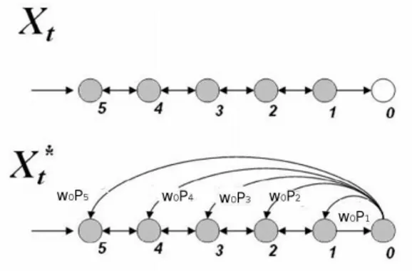
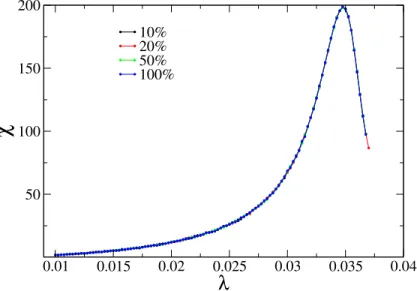
3.3 Original processXtwith an absorbing staten= 0and its related processXt∗. . . . 37 3.4 Susceptibility against infection rate for SIS model on a single network for different

sizes. . . 39

(15)

3.5 Susceptibility versus infection rate for the SIS model on a single network with

different initial conditions. . . 39

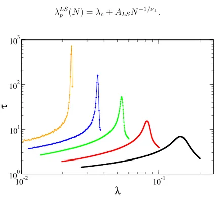
3.6 Lifespan versus infection rate for the SIS model on a single network for different sizes. . . 40

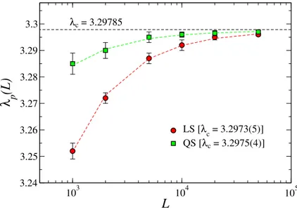
3.7 Size dependence of the λp(L)estimates for the transition point for the QS and LS methods. . . 41

4 Pair Approximation for the CP on Networks 42 4.1 Thresholds versus network size for the CP on UCM networks for PHMF and PQMF theories. . . 48

4.2 Thresholds versus network size for the CP on UCM networks. . . 49

4.3 Susceptibility versus creation rate. . . 50

4.4 Ratios between the factor˜gandgobtained in pair HMF theory. . . 55

4.5 FSS of the characteristic time and critical QS density. . . 56

5 Pair Approximation for the SIS Model on Complex Networks 58 5.1 Simple graphs used to study SIS dynamics under pair QMF theory. . . 60

5.2 Susceptibility versus infection rate for SIS model on RRNs. . . 61

5.3 Susceptibility versus infection rate for star graphs. . . 63

5.4 Susceptibility versus infection rate for wheel graphs. . . 64

5.5 Thresholds versus network size for SIS model on UCM network. . . 65

5.6 The same analysis of Fig. 5.5 forγ = 2.75. . . 66

5.7 Thresholds versus network size for the SIS model on random networks. . . 67

6 Multiple transitions of the SIS Model on Complex Networks 70 6.1 Numerical determination of the thresholds for the SIS model on UCM networks. . 72

6.2 (a) Susceptibility, (b) stationary density and (c) its logarithmic derivative versus infection rate for a SF networks . . . 74

(16)

6.3 PR as a function of the infection rate for the same networks and immunization strategies shown in Fig. 6.2. . . 75

6.4 (a) PR versus system size for a fixed distanceλ₋λp = 0.012. (b) The same analysis of panel (a) for QS density. . . 76

6.5 Thresholds for SIS dynamics on SF networks. . . 77

6.6 Left: Schematics of a double random regular network (DRRN). Right: Susceptibil-ity versus infection rate for DRRNs. . . 78

6.7 Threshold analysis for DRRN. . . 79

6.8 (a)The lifespan and (b) the QS density of infected vertices versus infection rate for SIS model on DRRNs. . . 80

6.9 Susceptibility (top) and QS lifespan (bottom) versus infection rate for SIS dynamics on a network. . . 81

6.10 (a) The tail of the degree distributions for networks with either rigid or natural cutoff. (b) QS density versus infection rate. . . 81

6.11 (a) Susceptibility curves for networks with rigid cutoff. (b) Threshold versus sys-tem size for rigid and natural cutoffs. . . 82

III Random Walks on Temporal Networks

85

7 Random Walks on Activity Driven Temporal Networks 85

7.1 Random walk process on activity driven networks. . . 86

7.2 Stationary density of a random walker in activity-driven network. . . 89

7.3 MFPT of a random walker as a function of the activity a in activity-driven network. 90

8 Slow Dynamics in Random Walks on Temporal Networks 91

8.1 Evolution towards equilibrium of the occupation probabilityP(a, tw). . . 94 8.2 Occupation probabilityP(a, tw)as a function of the activityaat different timestw. 95 8.3 Two-time correlation function for random walks on activity driven networks. . . . 98

8.4 Scaling plot of the average scape time. . . 99

(17)

8.5 Coverage as a function of time. . . 100

8.6 Evolution of the occupation probabilityP(a, t). . . 102 8.7 Scaling plot of the average scape time. . . 103

(18)

List of Tables

II Epidemics Spreading on complex networks

20 Pair Approximation for the Contact Process on Complex Networks

42

4.1 Transition points of the contact process on UCM networks with different degree exponents. . . 51

4.2 Critical exponents obtained in QS simulations of the CP on UCM networks. . . 55

(19)

RESUMO

MATA, Angélica Sousa da, M. Sc., Universidade Federal de Viçosa, Fevereiro de 2015. PRO-CESSOS EPIDÊMICOS E DIFUSÃO EM REDES: ABORDAGENS ANALÍTICA E COM-PUTACIONAL. Orientador: Silvio da Costa Ferreira Junior. Co-Orientadores: Marcelo Lobato Martins e Romualdo Pastor-Satorras.

Uma área de crescente interesse na Física Estatística é o estudo de processos dinâmicos em redes complexas. Neste contexto, o objetivo principal dessa tese é investigar o comportamento de proces-sos epidêmicos em redes heterogêneas. Com esse intuito, aprimoramos as teorias de campo médio

quenched e heterogênea através de aproximações de pares nas quais a correlação dinâmica entre

vértices vizinhos é explicitamente levada em considerção. Essas abordagens nos permitem determi-nar, com maior precisão, os limiares epidêmicos do modelo suscetível-infectado-suscetível (SIS), e também as relações de escala dos expoentes críticos associados à transição de fase para o estado absorvente no processo de contato (CP). Também investigamos a dinâmica do modelo SIS em re-des aleatórias com distribuição de conectividade em lei de potência (P(k) _∼ k−γ), com expoente γ > 3, uma vez que a existência ou ausência de um limiar finito envolvendo uma transição para

a fase endêmica tem sido alvo de muitos estudos recentemente. Encontramos que o modelo pode exibir múltiplas transições envolvendo epidemias localizadas. Nossa análise numérica também in-dica que a transição para uma fase endêmica pode ocorrer num limiar finito. Nossos resultados mostram que teorias de campo médio a princípio contraditórias, na verdade são complementares porque elas descrevem diferentes limiares epidêmicos que podem aparecer concomitantemente em uma única rede. Finalmente, nós também investigamos processos de difusão em redes temporais através do modelo de caminhada aleatória. Além de ser estudada numericamente via simulações, tal dinâmica também foi estudada teoricamente através do seu mapeamento no modelo de armadil-has de Bouchaud. Nesse estudo foram encontradas evidências do comportamento de aging na

relaxação de tal processo dinâmico.

(20)

ABSTRACT

MATA, Angélica Sousa da, M. Sc., Universidade Federal de Viçosa, February, 2015.EPIDEMIC PROCESSES AND DIFFUSION ON NETWORKS: ANALYTICAL AND COMPUTATIONAL APPROACHES. Adviser: Silvio da Costa Ferreira Junior. Co-Advisers: Marcelo Lobato Martins and Romualdo Pastor-Satorras.

A field of outstanding interest in Statistical Physics is the investigation of dynamical processes on complex networks. This thesis is devoted to explore the behavior of epidemic dynamics running on heterogeneous networks. We improved analytical approaches - quenched and heterogeneous mean-field theories - by means of pair approximations, which explicitly take into account dynam-ical correlations between connected vertices. These approaches yield more accurate predictions of the epidemic thresholds in the susceptible-infected-susceptible (SIS) model and the critical expo-nents associated to the absorbing state phase transition of the contact process (CP) obtained through finite-size scaling. These approaches can be applied to dynamical processes on networks in gen-eral providing a profitable strategy to analytically assess and fine-tune theoretical corrections. We also investigated the SIS dynamics on random networks having a power law degree distribution (P(k)_∼ k−γ_{), with exponent} _{γ >} ₃_{, since the existence or absence of a finite threshold involving} an endemic phase has been target of a recent and intense investigation. We found that this model on a single network can exhibit multiple transitions involving localized epidemics and our numerical analysis indicates that the transition to the endemic state occurs at a finite threshold. Our analy-sis points out that competing mean-field theories are, in fact, complementary since they describe different epidemic thresholds which can concomitantly emerge in a single network. Finally, we also investigated the diffusion processes on temporal networks by means of a random walk. We analyzed this dynamic theoretically by means of a mapping to Bouchaud’s trap model and using numerical simulations. We found evidence of aging behavior in the random walk relaxation.

(21)

Part I

(22)

Chapter 1 Introduction

There are many systems composed by a large number of elements connected according to a defined type of interactions. Examples can be found in different places present in our daily lives. The Internet is a collection of computers linked by data connections, the society consists of people linked by social relations, an ecosystem can be seen as a web of species connected by prey-predator relationships, our brain is constituted by a set of neurons connected by synapses, etc [1,2].

These examples have a common characteristic: they can be modeled as a network. The com-ponents of the system are the network vertices and the interactions among them are the edges [3]. These systems are often the scenario of interesting phenomena which can affect our routine. For instance, the Internet affects the way we access and produce information, the connections in a so-cial network affect how people form opinions, interact sexually, or make working partnerships, etc. Beyond that, there are some disasters that can happen if some failure occurs in these systems: breakdown of the power grid can leave cities without electricity for many hours, a failure of a global financial system can lead a national economy to collapse, the fast spreading disease due to a dense air transport network can cause an epidemic outbreak [4].

The empirical studies of real-world systems were motivated by such phenomena and gave rise a important area of Science: the theory of complex networks. This area has a highly multidisciplinary nature, being the object of study in many fields including mathematics, computer science, sociology and physics. Particularly, in statistical physics, it is useful to reduce a complex system to a network representation. Even though this approach cannot capture all details of the system, one can use a set of statistical tools for the analysis, modeling and characterization of networks and to make predictions about dynamical processes taking place on it [1,5–8].

(23)

1. Introduction 3

the aim of answering several questions [9–24]. How can we describe the network topology with a small set of descriptors? How can different system as technological and social networks have

similar connectivity patterns? How can the topology of the substrate affect the dynamics of the

process taking place on it? What happens to the system behavior if the network has an intrinsic

temporal dynamics?

Our current research, supported by many previous works, try to shed light on some of these questions. We review, in the first part of this thesis (chapter 2), the fundamental concepts that are used during all the text. A brief review to describe complex systems using a toolset of complex networks theory is presented. We show that graphs representing different systems can have com-mon features like heterogeneous topology, scale-free (SF) structure (their connectivity distribution follows power-law behavior), small-world property (vertices can be reached from every other with a small number of steps), etc [3,4,25,26] (section 2.1). We also present some static network mod-els emphasizing theuncorrelated configuration model(UCM) [27] (section 2.2.1) that is useful to

check the accuracy of analytical solutions of dynamical processes on networks. We also discuss the role of the intrinsic time-varying network on the dynamics running on top of it. Special attention is devoted to the activity driven networks[28] (section 2.2.2) since many studies about epidemic

spreading and diffusion have been reported in this class of temporal networks [24,29–32].

We divided the thesis in two other parts beyond this introductory one. The part II is devoted to the study of epidemic spreading on static networks, and the part III refers to diffusion processes on temporal networks.

In the part II, we firstly review the theory and modeling of non-equilibrium dynamical systems on networks (chapter 3). Particularly relevant in this context are processes that exhibit absorbing-state phase transitions [33,34]. In the epidemic scenario, individuals can be in both infected or susceptible states. A phase transition between a disease-free (absorbing) state and an active sta-tionary phase where a fraction of the population is infected are separated by an epidemic threshold

λc [5]. The susceptible-infected-susceptible (SIS) model and the contact process (CP) [35] rep-resent the simplest epidemic models possessing an absorbing-state phase transition (section 3.1). For the SIS model, the central issue of many recent works is to determine an epidemic threshold separating an absorbing, completely healthy state, from an active phase on heterogeneous net-works [11,13–16,36–39] (section 3.6). In turn, for the CP model, most of the interest relies on the relation between critical exponents and statistical properties of the network, in particular the degree distribution [21,22,40–43] (section 3.5).

(24)

1. Introduction 4

(HMF) approach [44] (section 3.4) for dynamical processes on complex networks has become widespread in the last decade. This theory, formerly conceived to investigate dynamical processes on complex networks, assumes that the number of connections of a vertex (the vertex degree) is the single quantity relevant to determine the state of the vertex, neglecting all dynamical correlations as well as the actual structure of the network. On the other hand, the quenched mean-field (QMF) theory [13,45] (section 3.3) still neglects dynamical correlations but the actual quenched structure of the network is explicitly taken into account by means of the adjacency matrix that contains the complete information of the connections among vertices [3].

However, neglecting dynamical correlations is an important drawback to ascertain the accuracy of the analytical results. The simplest way to explicitly consider dynamical correlations is by means of a pair-approximation [34]. In chapters 4 and 5, we present our original contribution to this topic by means pair QMF and HMF approximations for the CP [46] and SIS [39] models on heterogeneous networks.

In order to check the predictions of these theories, numerical investigations of the SIS and CP models on several networks have been recently reported [13,36,42,43,47–49]. Also in chapter 3 we present simulations techniques used to analyzed both models numerically. Numerical recipes for the simulation of Markovian epidemic models on complex networks can be found with more details in the Ref. [50], in which we present distinct algorithms and compare their computational efficiency (section 3.7.1).

To overcome the difficulties intrinsic to the stationary simulations of finite systems with absorb-ing states we use a robust approach called quasi-stationary (QS) method [51] (section 3.8.1). All simulations performed in chapters 4 and 5 we are done using this technique. However, recently, Boguñáet al.[16] proposed a new strategy, called lifespan (LS) method, in which the simulation

starting from a single infected vertex and a diverging epidemic lifespan was used as a criterion to determine the thresholds (section 3.8.2). In Ref. [52], we check the feasibility of this method and conclude that it is an alternative way to numerically study systems with absorbing states.

Particularly, the existence or absence of finite epidemic thresholds involving an endemic phase of the SIS model on scale-free networks with a degree distribution P(k) _∼ k−γ_{, where}_γ _{is the} degree exponent, has been target of a recent and intense investigation [11,13,15,16,36,38,53] (sec-tion 3.6). Distinct theoretical approaches for the SIS model were devised to determine an epidemic threshold produced different outcomes. The HMF theory predicts a vanishing threshold for the SIS model for the range2< γ _≤3while a finite threshold is expected forγ >3. Conversely, the QMF

(25)

1. Introduction 5

Motivated by controversial discussions [11,15,16,54,55], in chapter 6, we performed extensive simulations for the SIS dynamics on SF networks with exponentγ >3. We found that a much more complex behavior with multiple transitions can arise from this dynamic. In individual networks with large gaps in the degree distribution we can observe multiple epidemic thresholds that are well described by different mean-field theories.

Finally, in the part III of this thesis, we advance in the study of networks considering now its temporal property. In the part II, we shown that the heterogeneous topology of a complex network [3] can have a relevant impact on the properties of dynamical systems running on top of it [1,26]. However, many dynamical effects can take a different, more complex turn when one considers the intrinsic time-varying,temporalnature of many real networks [56]. Indeed, networked systems are

often not static, but show connections which appear and disappear during some characteristic time scales that can be of the same order of magnitude as those ruling a dynamical process on networks. Social networks [7] represent the prototypical example of this behavior, being defined in terms of a sequence of social contacts that are continuously established and broken. This mixing of time scales can induce new phenomenology on the dynamics of temporal networks, in stark contrast with what is observed in static networks [24,29,32].

(26)

Chapter 2 Fundamentals of Network Theory

The study of complex networks is inspired by empirical analysis of real networks. Indeed, com-plex networks allow us to understand various real systems, ranging from communication networks to ecological webs [25]. In general terms, a network is a system that can be represented as a graph, composed by elements called nodes or vertices and a set of connecting links (edges) that represent the interactions among these elements [2] (Figure 2.1).

Figure 2.1: An example of a simple graph.

The advantage of modeling a system as a graph is that networks provide a theoretical frame-work that allows a suitable representation of interactions in complex systems. For instance, our brain is made up of a set of neurons connected by synapses, the Internet is formed by routers and computers cables and optical fibers, the society consists of people connected by social relationships as scientific collaboration, friendship, etc. [1,25,58].

(27)

2. Fundamentals of Networks Theory 7

theory. On the other hand, the study of very large systems requires a statistical characterization. In this chapter, we provide a brief introduction to the basic notions and notations of network theory which are used throughout this thesis. To conclude this short review, we will describe, in last sec-tion, network models that can be used to study dynamical processes in the context of computational approaches. Particular emphasis will be devoted to uncorrelated configuration model (UCM) and activity driven network, since the first one was used in this thesis to study epidemic spreading on static networks (PartII) and the latter was used to investigate slow dynamics on temporal networks (PartIII).

2.1 Basic Concepts and Statistical Characterization of Networks

From a mathematical point of view, we can represent a network by means of an adjacency matrix_A. A graph ofN vertices has aN _×N adjacency matrix. The edges can be represented by

the elementsAij of this matrix such that [2]

Aij =

(

1, if the verticesiandj are connected

0, otherwise (2.1)

The concept of adjacency matrix is very useful in quenched mean-field theory that explicitly takes into account the actual connectivity of the network [13,45]. This issue is discussed with more details in section 3.3 of Part II.

A relevant information that can be obtained from the adjacency matrix is the degree ki of a vertexidefined as the number of edges attached to the vertexi,i.e., the number of nearest neighbors

of the vertexi. The degree of the vertices can be written by means of the adjacency matrix as [2] ki =

N

X

j=1

Aij. (2.2)

A central issue in the structure of a graph is the reachability of its vertices,i.e., the possibility

that any information goes from one node to another through a path formed by the edges in the network [1]. For instance, we have a gossip spreading in a social network or a nerve impulse propagating in a neural network [2].

A path_Pij is defined as an ordered collection ofn+ 1vertices connected bynedges in a such a way that connect the verticesiandj. The concept of path leads us to define the distance between

(28)

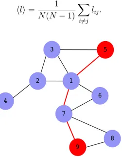
of edges in the shortest connecting path denoted asℓij (see figure 2.2). The average shortest path length is defined as the value ofℓij averaged over all the possible pairs of vertices in the network such that [59]

hl_i= 1

N(N ₋1) X

i6=j

lij. (2.3)

Figure 2.2: A network where the shortest path connecting two different vertices (5and9) is

high-lighted.

Typically, the number of neighbors in a complex network at a distanceℓcan be approximated by_hk_iℓ_{, considering that each vertex has degree equal to the average degree of the network}_h_k_i_[see definition below - Eq. (2.7)] and there is no loop1_{. Since the quantity}

hk_iℓ_{rapidly grows with}_ℓ_{, we} can thus roughly estimate_hℓ_iby the condition_hk_iℓ _∼_N_{, then [1,59]}

hℓ_{i ≃} lnN

ln_hk_i. (2.4)

For a d₋dimensional lattice, the number of neighbors at a distance ℓ scales as ℓd_{, implies} that _hℓ_{i ∼} N1/d_{. So, the growth of} _h_ℓ_i _{slower than any positive power of} _N _{characterizes the} network with the small-world property2 _{[1]. This scaling behavior is observed in many real-world}

phenomena, including websites, food chains, metabolite processing networks, etc [2,25,58].

Beyond the small-world characteristic, a network can be also described by the structure of the neighborhood of a vertex. The tendency to form cliques (fully connected sub-graphs) in the

1_{A loop or a cycle is a closed path}_P_ij(_i₌_j₎_{in which all nodes and all edges are distinct [2].}

(29)

neighborhood of a given vertex is observed in many natural networks; for example, a group of friends who know each other. This property is called clustering and implies that if the vertexiis connected to the nodej, and this one is connected tol, there is a high probability that i is also

connected tol. The clusteringC(i)can be measured as the relative number of connections among

the neighbors ofi[59]:

C(i) = ni

ki(ki−1)/2

. (2.5)

Hereki is the degree of the nodeiandniis the total number of edges among its nearest neigh-bors. The mean clustering coefficient is given by:

hC_i= 1

N

X

i

C(i). (2.6)

Apart from small-world and clustering properties, looking at very large systems as a protein network or the World Wide Web, an appropriate description can be done by means of statistical measures as the degree distributionP(k). The degree distribution provides the probability that a

vertex chosen at random haskedges [25,60].

The average degree is given by the average value ofkover the network,

hk_i= 1

N

X

i=1

ki =

X

k

kP(k). (2.7)

Similarly, it is useful to analyze then-thmoment of the degree distribution [1]

hkn_i₌X

k

kn_P₍_k₎_. _(2.8)

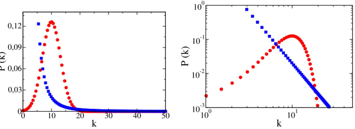
We can classify networks according to their degree distribution. The basic classes are homo-geneous and heterohomo-geneous networks. The first ones exhibit a fast decaying tail, as for example, a Poisson distribution. Here the average degree value corresponds to the typical value in the system. On the other hand, heterogeneous networks exhibit heavy tail that can be approximated by a power-law decay,P(k)_∼ k−γ. In this second case, the vertices will often have a small degree, but there

is a non-negligible probability of finding nodes with very large degree values thus, depending onγ,

(30)

0 10 20 30 40 50

k 0 0,03 0,06 0,09 0,12 P (k)

100 101

k 10-3 10-2 10-1 100 P (k)

Figure 2.3: Comparison of a Poisson (circles) and a power law withγ = 3(squares) degree distributions

on a linear (left) and a double logarithmic plot (right). Both distributions have the same average degree hk_i= 10.

The role of the heterogeneity can be understood by looking at the first two moments of a power law distributionP(k)_∼k−γ. We can compute the average degree value as3:

hk_i=

Z kmax

k0

kP(k)dk, (2.9)

wherek0 ≥1is the lowest possible degree in the network andkmaxis the maximal degree observed (upper cut-off of the distribution). Computing the integral one has [1],

hk_i=

Z kmax

k0

kAk−γdk = Ak 2−γ

2₋γ

kmax k0

≈ (γ−1)

(γ₋2)k0 (2.10)

forkmax → ∞ and for γ > 2. The normalization constant is given by A ≃ (γ −1)k0γ−1. We observe that the average degree is well defined and finite. The statistical fluctuations present in the system can be expressed by the normalized variance of the distributionσ2_/_h_k_i2 _{whose main} contribution is given by the second moment,

hk2_i=

Z kmax

k0

k2Ak−γdk _∼

(

k3−γ

max, if 2< γ <3

const., if γ >3. (2.11)

In the thermodynamic limit, _hk2_{i → ∞}_{, for} ₂ _{< γ} _≤ ₃_{. This means that the fluctuations} around the average degree are unbounded. We observe a scale free network since the absence of any intrinsic scale for the fluctuations implies that the average degree is not a characteristic scale for the system [25,59]. However, forγ _≥3, the second moment remains finite. Indeed, besides the

3_{For simplicity, it is usual consider}_k_{a continuous variable. However when the integral is replaced by a discrete}

(31)

shape of the power law degree distribution, we shall see further that the exponentγ has profound implications on dynamical processes running on top of heterogeneous substrates.

Other typical feature of networks is the tendency of nodes with a given degree connect with nodes with similar or dissimilar degree. When high or low degree vertices connect to other vertices with similar degree with higher probability, one says the correlations presented in the network are assortative. Conversely, if nodes of different degree are more likely to attach, the correlations are called disassortative [61].

One way to quantify the degree correlations is in terms of the conditional probabilityP(k′_|_k₎ that a node with degreekis connected with a vertex with degreek′ _{[1]. Since to determine}_P₍_k′_|_k₎ can be a rather complicated task, a simple approach is given by the average degree of the nearest neighbors (NN) of a vertexiwith degreeki[62],

knn,i =

1

ki

X

j∈N(i)

kj, (2.12)

where the sum runs over by the nearest neighbors vertices ofi. Then, the behavior of the degree

correlations is obtained by the average degree of the nearest neighbors, knn(k), for vertices of degreek[63]:

knn(k) =

1

Nk

X

i/ki=k

knn,i, (2.13)

whereNkis the number of nodes of degreekand the sum runs over all vertices with the same degree

k. This quantity is related to the correlations between the degrees of connected nodes because in average it can be expressed as

knn(k) =

X

k′

k′P(k′_|k). (2.14)

If degrees of neighboring vertices are uncorrelated,P(k′_|_k₎_{is just a function of}_k′ _and_k

nn(k)is a constant. Ifknn increases withkthen vertices with high degrees have a larger likelihood of being connected to each other. On the other hand, if knn decreases with k, high degree vertices have larger probabilities of have neighbors with low degrees [1,27,63] (See figure 2.4).

2.2 Networks Classes

(32)

Figure 2.4: Schematic representation of the (a) assortative, (b) disasortative and (c) uncorrelated properties of the network indicated by the behavior of the average degree of the nearest neighbors,

knn, for vertices with degreek.

patterns of connections between parts of systems such as Internet, power grid, food webs, social networks, etc [2,58,64].

On the one hand, technological networks as Internet are physical infrastructure networks that can be represented by static networks,i.e., the nodes and edges are fixed or change very slowly over

time [3]. On the other hand, networks that describe some form of social interaction between people have an intrinsic time-varying nature that should be taken into account. For instance, in a scientific collaboration network, the authors are not in contact with all their collaborators simultaneously during all the time. Indeed, real contact networks are dynamic with connections that appear and disappear with different characteristic time scales [28,56].

From the viewpoint of dynamical processes, both classes of networks static and temporal -are important. The first one has been widely studied and it is convenient for analytical tractability whereas the second one is more realistic and constitutes a very promising approach. According to the development of complex networks over the years, we will start discussing the static networks and on the sequence the temporal ones.

2.2.1 Static Networks

The simplest prototype of a network was investigated by Erd˝os and Rényi, in 1959 [65]. In its original formulation, a graph is constructed starting from a set ofN nodes and all edges among

them have the same probability of existing.

Afterwards, in 1998, Watts and Strogatz (WS) proposed a more realistic model inspired by social networks that became known as thesmall-world model[10]. WS networks are constructed

(33)

connected networks and conserves the number of edges (_hk_i =m). However, even at smallp, the emergence of shortcuts among distant nodes greatly reduces the average shortest path length.

Concomitantly, Barabási and Albert [9] proposed a preferential attachment model suited to reproduce the feature of time growth of many real networks. In this model, new vertices are added to the system at every step. Each new vertice is connected to those nodes already present in the network with a probability proportional to their degrees at that time. The properties of growth and preferential attachment are suitable to model realistic networks as the Internet and the World Wide Web [2,58]. This class of networks provides an example of the emergence of graphs with a power law degree distribution [P(k)_∼k−γ_{] and small-world properties.}

In addition to their power law degree distributions, real networks are also characterized by the presence of degree correlations reflected on their conditional probabilities P(k′_|_k₎ _{(see previous} section). For uncorrelated networks, P(k′_|_k₎ _{can be estimated as the probability that any edge} points to a vertex with degreek′, leading toPunc(k′|k) = k′P(k′)/hki[66]. Thus, using Eq. (2.14) the average nearest-neighbor degree becomes,

kunc_nn (k) = hk 2_i

hk_i2, (2.15)

that is independent of the degreek.

Although most real networks show the presence of correlations, uncorrelated random graphs are important from a numerical point of view, since we can test the behavior of dynamical systems whose theoretical solution is available only in the absence of correlations. For this propose, Catan-zaroet al.[27] proposed an algorithm to generate uncorrelated random networks with power law

degree distributions, called uncorrelated configuration model (UCM). The steps of the algorithm are the following:

(i) In a set of N disconnected vertices, each nodeiis signed with a numberki of stubs, where

kiis a random variable with distributionP(k)∼ k−γ under the restrictionsk0 ≤ki ≤N1/2

andP

iki even. It means that no vertex can have either a degree smaller than the minimum degreek0or larger than the cutoffkc =N1/2.

(ii) The network is constructed by randomly choosing two stubs and connecting them to form edges, avoiding both multiple and self-connections.

(34)

one expects that above a valuekcwe find of order of one vertex [64,67],

N

Z ∞

kc

P(k)dk _∼1. (2.16)

In this case, one obtains,

kc ∼N1/(γ−1), (2.17)

which is thenatural cutoffof the network [60]. However, for networks with power law degree

dis-tributions with2 < γ _≤3, it is possible to construct an uncorrelated network, without a structural

cut-off only if one permits multiple and self-connections, so that the constraint of forbidding these kind of connections introduces correlations in the network [27].

In order to shed light on this problem, we adapted some parts of Ref. [66], in which Boguñáet al. analyzed the degree distribution’s cutoff in finite size scale-free networks. Let us definerkk′ as

rkk′ = Ekk ′

mkk′

, (2.18)

whereEkk′is the number of edges between vertices of degreekandk′, andm_kk′ = min(kN_k, k′N_k′, N_kN_k′) is the maximum number of connections allowed between them, considering the restriction of not

having multiple edges. If multiples edges are instead allowed mkk′ is simply given by m_kk′ =

min(kNk, k′Nk′). Here,N_k =N P(k)is the number of vertices of degreek. Thus, the ratio can be written as [66]

rkk′ = hkiP(k, k ′₎

min[kP(k), k′_P₍_k′₎_{, N P}₍_k₎_P₍_k′_)], (2.19) since the joint distribution is defined as the probability that a randomly chosen edge connects two vertices of degreeskandk′, that yields [1]

P(k, k′) = Ekk′

hk_iN. (2.20)

For uncorrelated networks, the joint distribution can be factorized as

Punc(k, k′) =

kk′_P₍_k₎_P₍_k′₎

hk_i2 . (2.21)

We can observe that ifk > Nk′ andk′ > Nk, it is not possible to connect vertices with degrees

k and k′ _{with each other without multiples edges. Then} _min[_kP₍_k₎_{, k}′_P₍_k′₎_{, N P}₍_k₎_P₍_k′_{)] =}

N P(k)P(k′₎_{and the ratio}_r

(35)

rkk′ = kk ′

hk_iN. (2.22)

Independently of the type of the network, this ratio must be smaller than or equal to1. If one

considers the spacek ₋k′ _{in which the joint probability is defined, the curve} _r

kk′ = 1delimiting the regionrkk′ < 1, in which the pairs(k, k′)taking admissible values, from the regionr_kk′ > 1, physically forbidden (see Fig. 2.5). The structural cutoffksmust preserve this physical condition, so it can be defined as the value of the degree delimiting the largest square region of admissible values. That is given as the intersection of the curvesk =k′ _and_r

kk′ = 1. Thus,k_sis the solution of the implicit equation

rksks = 1. (2.23)

According Eq. (2.22), the structural cutoff takes the form

kc(N)∼(hkiN)1/2, (2.24)

for anyγ in the power law degree distribution [66]. For γ > 3, the constraint of the structural

cutoff is expendable since it diverges faster than the natural cutoff. However, scale-free networks (2 < γ _≤ 3) must posses a structural cutoff because the exponent of the natural cutoff is greater

than1/2, and consequently, it diverges faster than the structural one. Then, for UCM networks,

one has the cutoffkcscaling ashkci ∼N1/ω, whereω = max(2, γ−1)[27].

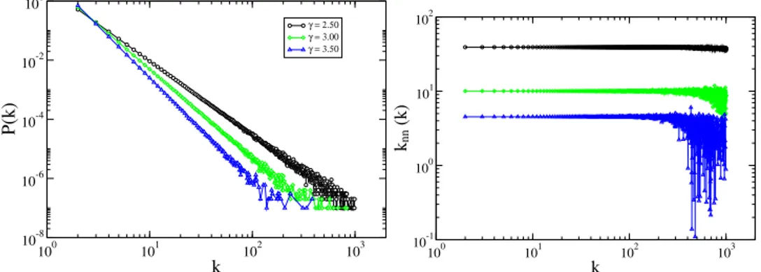
Figure 2.5: Geometrical construction of the structural cutoffkS. Taken from Ref. [66] In figure 2.6 we show a power law degree distribution for the UCM model [27] with different values of the degree exponentγand check the lack of correlations. We can observe a flat behavior

(36)

one obtains a random maximum degreekmax, with an average_hkmaxi=kc. Forγ >3, both mean and the standard deviation ofkmaxscale askc ∼N1/γ−1(see section 6.2 of Part II). As we can see in Fig. 2.6(b), this implies thatkmax has large fluctuations for different network realizations [69].

100 101 102 103

k

10-8 10-6 10-4 10-2 100

P(k)

γ = 2.50 γ = 3.00 γ = 3.50

100 101 102 103

k

10-1 100 101 102

knn

(k)

Figure 2.6: Power law degree distribution (left) and average nearest-neighbor degree of vertices of degree

k(right) for the UCM network with different degree exponentsγ, withN = 106 andk₀ = 2.

As said previously, this algorithm is very useful in order to check the accuracy of many analyt-ical solutions of dynamanalyt-ical process on networks. In particular, this model is used in the Part II of this thesis, where we numerically test the behavior of epidemic models taking place on the top of complex networks and compare them with analytical approximations that are available just in the absence of degree correlations.

2.2.2 Temporal Networks

As shown in the previous section, the network structure helps us to understand the behavior of dynamical systems. However, in many cases, the edges are not continuously active. For example, in communication networks via email, edges represent sequences of instantaneous contacts [56]. In closed gatherings of individuals such as schools and conferences the agents are not simultaneously establishing interactions in the system [70,71]. Similarly to the network topology, the intrinsic time evolution of the network can also affect the system’s dynamics from disease contagion to information diffusion [24,72,73].

Indeed, this mixing of time scales can induce new phenomenology on the dynamics on tempo-ral networks, in stark contrast with what is observed in static networks. Moreover, thebursty

(37)

Particularly relevant in this topic is the activity driven network [28]. Indeed, it represents a

class of social temporal network models based on the observation that the establishment of social contacts is driven by the activity of individuals, prompting them to interact with their peers at different levels of intensity. Based on the empirical measurement of heterogeneous levels of activity denoted bya, across different datasets, activity strength has been found to be distributed according

to a power law form,F(a)_∼a−γ[28].

The activity driven network model proposed by Perra et al. [28] is defined as follows (See

figure 2.7):N nodes (individuals) in the network are endowed with an activityai ∈[ε,1], extracted randomly from an activity distributionF(a). Every time step∆t = 1/N, an agentiis uniformly chosen at random. With probability ai, the agent becomes active and generates m links that are connected tomother agents, uniformly chosen at random. Those links last for a period of time∆t

(i.e.are erased at the next time step). Time is updated ast_→t+ ∆t. The topological properties of

the integrated network at timet(i.e. the network in which nodesiandj are connected if there has

ever been a connection between them at any timet′ _≤t) were studied in Ref. [82]. The main result

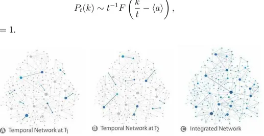
is that the integrated degree distribution at timet, Pt(k), scales in the larget limit as the activity distribution, i.e.

Pt(k)∼t−1F

k t − hai

, (2.25)

consideringm= 1.

Figure 2.7: Schematic representation of the activity driven network model. We show a visualization of the resulting networks for 2 different time steps and the last visualization represents the integrated network. Figure taken from Ref. [73].

Empirical measurements report activity distributions in real temporal networks exhibiting heavy tails of the formF(a)_∼a−γ _{[28]. This expression thus relates in a simple way the functional form} of the activity distribution and the degree distribution of the integrated network at timet, and allows to explain the power-law form of the latter observed in social networks [83].

(38)

appli-2. Fundamentals of Networks Theory 18

cations - a time-varying substrate can induce noticeable differences with respect to the behavior expected in static networks [24,29–31]. We will consider activity distributions with a power-law form. The range of values of thea is restricted toa _∈ [ε,1], where a minimum activityεis set to

avoid divergences. As we will see inchapter8 -PartIII, the parameterεwill play a significant role

(39)

Part II

(40)

Chapter 3 Phase Transitions with Absorbing States in

Complex Networks

The present chapter provides a short review of the modeling and theory of non-equilibrium dynamical systems on networks. A key class of non-equilibrium process are those that exhibit absorbing states,i.e.states from which the dynamics cannot escape once it has fallen onto them.

A relevant feature of many systems with absorbing states is the absorbing-state phase transi-tions [33,34], i.e. non-equilibrium phase transitions between an active state, characterized by an

everlasting activity in the thermodynamic limit, and an absorbing state, in which activity is absent.

The same type of transition occurs in epidemic spreading processes [5] since a fully healthy state is absorbing in the above sense, provided that immigration of infected individuals is not al-lowed. The susceptible-infected-susceptible (SIS) model and the contact process (CP) [35] repre-sent the simplest epidemic models possessing an absorbing-state phase transition.

Lattice systems that exhibit such absorbing state phase transitions have universal features, de-termined by conservation laws and symmetries which allow to group them in a same universality class1 _{[85]. The most robust class of absorbing state phase transitions is the directed percolation}

(DP) that was originally introduced as a model for directed random connectivity [86]. Both CP and SIS models are interacting particle systems involving self-annihilation and catalytic creation of particles that presents an absorbing-phase transition and thus belong to DP class. The SIS dynamics is indeed the most studied model to describe epidemic spreading on networks. Although the CP was initially thought as a toy model for epidemics [35], lately it has been widely used as a generic reaction-diffusion model to study phase transition with absorbing states.

1_{Once a set of models share the same symmetry properties, irrespective of the microscopic details of their dynamical}

(41)

3. Phase Transitions with Absorbing State in Complex Networks 21

Thus, this chapter is devoted to review the SIS and CP models as examples to investigate ab-sorbing phase transitions in complex networks. We firstly describe both epidemic models and, after we present distinct theoretical approaches devised for them. Finally we described the simulation techniques used to analyze both models numerically. For the SIS model, the central issue is to determine an epidemic threshold separating an absorbing, disease-free state from an active phase on heterogeneous networks [11,13–16,36–39]. While for the CP model, most of the interest is to relate the critical exponents with statistical properties of the network, in particular the degree distribution [21,22,40–43].

3.1 Epidemic Models

In the SIS epidemic model, each vertex i of the network can be in only one of two states: infected or susceptible which are represented by σi = 1 or σi = 0 respectively. Let us assume the most general case where a vertexibecomes spontaneously healthy at rateµi, and transmits the infection to each one of itski neighbors at rateλi. In figure 3.1, we show an example of the rates for a epidemic model. For classical SIS, one hasµi =µandλi =λfor every vertex.

Figure 3.1: The rates in the dynamics of the SIS model for a vertexiinitially infected.

As in the SIS model, vertices in the CP can be infected or susceptible, which in reaction-diffusion system’s jargon are called occupied (σi = 1) and empty (σi = 0), respectively. The spontaneous cure process is exactly the same as in the SIS model: infected vertices become sus-ceptible at rateµi =µ. The infection is, however, different. An infected vertex tries to transmit the infection to a randomly chosen neighbor at rateλ, implying that the transmission rate of vertexiis

λi = λ/ki, what reduces drastically the infective power of very connected vertices in comparison with the SIS dynamics.

(42)

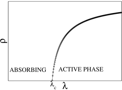
separated by an epidemic threshold λc. The density of infected nodes ρ is the order parameter that describes this phase transition, as shown in Figure 3.2. For heterogeneous networks a more complex behavior can emerge as discussed in chapter 6. However, for a finite system the unique true stationary state is the absorbing state, even above the critical point, due to dynamical fluctuations. To overcome the difficulty to study the active state of finite systems some simulation strategies were proposed in the literature, as we will see in the section 3.8.

The accurate theoretical understanding of epidemic processes running on the top of complex networks rates among the hottest issues in complex network theory [11,13–22,39]. Much effort has been devoted to understand the criticality of the absorbing state phase transitions observed in CP [20–22,40,41] and SIS [11,13–16,19,39] models, mainly based on perturbative approaches (first order inρ) around the transition point [11,13,14,18,21,39]. In the following we will present the basic mathematical approaches for the epidemic dynamics. Generally all these theories aim at understanding the properties of epidemics in the equilibrium or long term steady state, the existence of a non-zero density of infected individuals, the presence or absence of a threshold, etc. We will start with the simplest case namely the homogeneous mean-field theory, and thereafter we will review other more sophisticated mathematical approaches.

λ

ρ

ACTIVE PHASE

ABSORBING

λ

_c

(43)

3.2 Homogeneous mean-field theory

The prediction of disease evolution can be conceptualized within a variety of mathematical approaches. The simplest theory of epidemic spreading assumes that the population can be divided into different compartments according to the stage of the disease (for example, susceptible and infected in both SIS and CP models) and within each compartment, individuals (vertices in the complex networks’ jargon) are assumed to be identical and have approximately the same number of neighbors (edges),k_{≈ h}k_i[87]. The idea is to write a time evolution equation for the number of infected individualsI(t), or equivalently the corresponding densityρ(t) = I(t)/N, whereN is the

total number of individuals. For example, the equation describing the evolution of the SIS model is:

dρ(t)

dt =−µρ(t) +λhkiρ(t)[1−ρ(t)], (3.1)

considering uniform infection and cure rates (λi = λ and µi = µ, ∀ i = 1,2,· · ·N). The first term on the right-hand side of the Eq. (3.1) refers to the spontaneous healing and the second one to the infection process, that is proportional to the spreading rateλ_hk_i, the density of the susceptible vertices1₋ρ(t)that may become infected, and the density of infected nodesρ(t)in contact with any susceptible individual. Note that the evolution of the SIS model is completely described by Eq. (3.1), since the density of susceptible individualsS(t)/N = 1₋ρ(t). The mean-field character

of this equation comes from the fact that we have neglected the density correlations among different nodes. Thus, the probability that one infected vertex is connected to a susceptible one is approached asρ(t)[1₋ρ(t)].

Near the phase transition between a disease-free (absorbing) state and an active stationary phase we can assume that the number of infected nodes is smallρ(t) _≪ 1. In this regime, we can use a linear approximation neglecting allρ2 _terms2_{. So the Eq. (3.1) becomes}3_:

dρ(t)

dt =−ρ(t) +λhkiρ(t). (3.2)

The solution isρ(t) _∼ e−(1−λhki)t_{, implying that}_ρ _{= 0} _{is an stable fixe point for} ₁₋_λ_h_k_i _> ₀_. Thus, one obtains,

λc =

1

hk_i. (3.3)

Here, λc is the epidemic threshold such that for any infection rate above this value the epidemic lasts forever.

2_{Indeed, this equation can be exactly integrated, but we prefered this stability analysis approach that is uses in more}

complex theories in the next sections

(44)

Similar analysis can be done for the CP model. In this case, the homogeneous mean-field equation read as

dρ(t)

dt =−ρ(t) +λρ(t)[1−ρ(t)], (3.4)

since the transmission rate of each node isλ/_hk_i. Performing the same linear stability analysis in

the steady-state, one obtainsλc = 1.

In this framework, one considers that the connectivity patterns among individuals are homo-geneous, neglecting the highly heterogeneous structure of the contact network inherent to real systems [25]. Many biological, social and technological systems are characterized by heavy tailed distributions of the number of contactskof an individual (the vertex degree, in the network jargon), for such systems the homogeneity hypothesis is severely violated [1,3,25]. Complex networks are, in fact, a framework where the heterogeneity of the contacts can be naturally afforded [25]. In-deed, this heterogeneity plays the main role in determining the epidemic threshold. To take it into account, other approaches have been proposed. As we shall see in the next sections, the major aim is to understand how the spreading epidemic can be strongly influenced by the topology of the networks.

3.3 Quenched Mean-field Theory

The quenched mean-field (QMF) theory [13] explicitly takes into account the actual connectiv-ity of the network through its adjacency matrix. The central idea is to write the evolution equation for the probabilityρi(t)that a certain nodeiis infected. For the SIS model the dynamical equation for this probability takes the form [13]:

dρi

dt =−ρi+λ(1−ρi)

N

X

j=1

Aijρj. (3.5)

where Aij is the adjacency matrix that assumes Aij = 1 if vertices i and j are connected and

Aij = 0, otherwise [see equation (2.1) in chapter 2]. The first term on the right-hand side considers nodes becoming healthy spontaneously while the second one considers the event that the nodeiis healthy and gets the infection via a neighbor node.

Performing a linear stability analysis around the trivial fixed pointρi = 0, one has

dρi

dt =

X

j

(45)

where the Jacobian matrix is

Lij =−δij+λAij, (3.7)

δij being the Kronecker delta symbol. The transition occurs when the fixed point loses stability or, equivalently, when the largest eigenvalue of the Jacobian matrix isΥm = 0 [88]. The largest of

Lij is given by Υm = −1 +λΛm whereΛm is the largest eigenvalue of Aij. Since Aij is a real non-negative symmetric matrix, the Perron-Frobenius theorem states that one of its eigenvalues is positive and greater than, in absolute value, all other eigenvalues, and its corresponding eigenvector has positive components. So, one obtains the epidemic threshold of the SIS model in a QMF approach [13]:

λqmf_c = 1/Λm, (3.8)

where Λm is the largest eigenvalue of the adjacency matrix. For the CP dynamic, the Eq. (3.5) becomes,

dρi

dt =−ρi+λ(1−ρi)

X

j

Aijρj

kj

. (3.9)

Performing the same linear stability analysis around the trivial fixed point, as was done for the SIS model, one obtains

dρi

dt =

X

j

Lijρj, (3.10)

where the Jacobian matrix is given by

Lij =−δij +

λAij

kj

. (3.11)

Once again the transition point is defined when the absorbing phase becomes unstable or, equiva-lently, when the largest eigenvalue ofLijis null [88]. The largest ofLij is given byΥm =−1+λΛm whereΛm is the largest eigenvalue of Cij = Aij/kj. Notice thatvi = ki is an eigenvector ofCij with eigenvalueΛ = 1. Now, supported by the Perron-Frobenius theorem [3], we conclude that

the largest eigenvalue ofCij isΛm = 1 resulting in the transition pointλc = 1, as obtained in a homogeneous approximation.

Returning to the SIS model, the equation (3.8) can be complemented with the results of Chung

et. al.[89] who calculated the largest eigenvalue of adjacency matrix of networks with a power law

degree distributions as

Λm ≃

( √

kc, γ >5/2 hk2

i

hki, 2< γ <5/2

(3.12)

(46)

law degree distributions even when _hk2_i_{remains finite [89]. Therefore, the epidemic thresholds} scale as [49]

λc ≃

(

1/√kc, γ >5/2 hki

hk2_i, 2< γ < 5/2

(3.13)

which vanishes for any power-law degree distribution The reasons for this difference ofλcpredicts by QMF approach, forγlarger or smaller than5/2are explained in ref. [49]. In processes allowing endemic steady-states, the activation mechanisms depend on the degree of heterogeneity of the network. Forγ >5/2the hub sustains activity and propagates it to the rest of the system while for

γ <5/2the innermost network core collectively turns into the active state maintaining it globally.

However, the behavior of the SIS model on random networks with power-law degree distribution can be much more complex than previously thought. Multiple phase transitions can arise depending on the connectivity distribution of the network. We studied this issue thoroughly and our original results are reported in the chapter 6.

3.4 Heterogeneous Mean-Field Theory

In a HMF theory, dynamical quantities, as the density of infected individuals in the SIS model, depend only of the vertex degree and do not of their specific location in the network. Actually, the HMF theory can be obtained from the QMF one performing a coarse-graining where vertices are grouped according to their degrees. To take into account the effect of the degree heterogeneity we have to consider the relative densityρk(t)of infected nodes with a given connectivity k, i.e., the probability that a node withk links is infected. Again using the SIS model as an example, the dynamical mean-field rate equation describing the system can thus be written as [44]:

dρk(t)

dt =−ρk(t) +λk[1−ρk(t)]

X

k′

P(k′_|k)ρk′(t), (3.14) The first term on the right-hand side considers nodes becoming healthy at unitary rate. The second term considers the event that a node with k links is healthy and gets the infection via a nearest neighbor. The probability of this event is proportional to the infection rateλ, the number of con-nectionsk and the probability that any neighbor vertex is infected P(k′_|_k₎_ρ

k′. The linearization Eq. (3.14) gives

dρk

dt =

X

k

(47)

whereLkk′ =−δ_kk′+λkP(k′|k). Therefore, the epidemic threshold is

λc =

1 Λm

, (3.16)

whereΛm is the largest value ofCkk′ =kP(k′|k).

It is difficult to find the exact solution forΛm for a general form of P(k′|k). But it is possible to extract the value of the epidemic threshold. In the case of uncorrelated networks, P(k′_|_k_{) =}

k′_P₍_k′₎_/_h_k_i _and_C

kk′ = k′kP(k′)/hki. So, it is easy to check thatv_k = k is an eigenvector with eigenvalue_hk2_i_/_h_k_i_{that, according to Perron-Frobenius theorem, is the largest. Thus, we obtain} the epidemic threshold:

λhmf

c =hki/hk2i, (3.17)

Equation (3.17) has strong implications since several real networks have a power law degree distributionP(k) _∼ k−γ _{with exponents in the range}₂ _{< γ <} ₃_{[25]. For these distributions, the} second moment_hk2_i_{diverges in the limit of infinite sizes implying a vanishing threshold for the SIS} model or, equivalently, the epidemic prevalence for any finite infection rate. Both theories HMF and QMF predict vanishing thresholds for γ < 3 despite of different scaling for 5/2 < γ < 3.

However, while HMF predicts a finite threshold for networks with γ > 3, QMF still predicts a

vanishing threshold [49].

For the CP model, the heterogeneous mean-field equation, analogous to Eq. (3.14), can be written as

dρk(t)

dt =−ρk(t) +λk[1−ρk(t)]

X

k′

P(k′_|_k₎_ρ k′(t)

k′ . (3.18)

(48)

3.5 Finite Size Scaling for CP model on heterogeneous networks

In Ref. [43], Castellano and Pastor-Satorras derived the HMF theory for the CP dynamic in the limit of infinite network size. They obtained the following scaling

¯

ρ_∼(λ₋λc)β, β = max

1, 1

γ₋2

. (3.19)

At the transition pointλ=λc,

ρ_∼t−δ, δ =β. (3.20)

Also the relaxation time scales as

τ _∼(λ₋λc)−νk, νk = 1. (3.21)

These exponents are also obtained using a pair HMF approximation as we shall show in section 4.4.1.

Its predictions could not be directly checked against numerical simulations because of the presence of finite-size effects. A comparison became possible using the finite-size scaling (FSS) ansatz [92], adapted to the network topology, and they concluded that CP dynamics on networks was not described by the HMF approximation. However, it was assumed in Ref. [43] that het-erogeneous networks follows the same FSS known for regular lattices [34]. Indeed, the FSS on networks is more complicated than previously assumed. The behavior of the CP on networks of finite size depends not only on the number of verticesN but also on the moments of the degree

distribution [21]. This implies that, for scale-free networks, the scaling around the critical point depends explicitly on how the largest degreekcdiverges with the system sizeN. Such dependence introduces very strong corrections to scaling. However, if such corrections are properly taken into account, it is possible to show that the CP on heterogeneous networks agrees, with high accuracy, with the predictions of HMF theory [41].

Starting from Eq. (3.18), and considering, in addition, uncorrelated networks with P(k_|k′_{) =}

kP(k)/k, the overall densityρ=P

kρkP(k), obeys the equation [42]

dρ(t)

dt =ρ(t) +λρ(t)

"

1_{− h}k_i−1X

k

kP(k)ρk(t)

#

. (3.22)

Epidemic processes and diffusion on networks: analytical and computational aproaches

ANGÉLICA SOUSA DA MATA