www.atmos-chem-phys.net/16/6285/2016/ doi:10.5194/acp-16-6285-2016
© Author(s) 2016. CC Attribution 3.0 License.
Evaluating the impact of built environment characteristics on urban
boundary layer dynamics using an advanced stochastic approach
Jiyun Song and Zhi-Hua Wang
School of Sustainable Engineering and the Built Environment, Arizona State University, Tempe, AZ 85287, USA
Correspondence to:Zhi-Hua Wang ([email protected])
Received: 23 November 2015 – Published in Atmos. Chem. Phys. Discuss.: 24 February 2016 Revised: 21 April 2016 – Accepted: 10 May 2016 – Published: 24 May 2016
Abstract. Urban land–atmosphere interactions can be cap-tured by numerical modeling framework with coupled land surface and atmospheric processes, while the model perfor-mance depends largely on accurate input parameters. In this study, we use an advanced stochastic approach to quantify parameter uncertainty and model sensitivity of a coupled nu-merical framework for urban land–atmosphere interactions. It is found that the development of urban boundary layer is highly sensitive to surface characteristics of built terrains. Changes of both urban land use and geometry impose sig-nificant impact on the overlying urban boundary layer dy-namics through modification on bottom boundary conditions, i.e., by altering surface energy partitioning and surface aero-dynamic resistance, respectively. Hydrothermal properties of conventional and green roofs have different impacts on at-mospheric dynamics due to different surface energy parti-tioning mechanisms. Urban geometry (represented by the canyon aspect ratio), however, has a significant nonlinear im-pact on boundary layer structure and temperature. Besides, managing rooftop roughness provides an alternative option to change the boundary layer thermal state through modifica-tion of the vertical turbulent transport. The sensitivity analy-sis deepens our insight into the fundamental physics of urban land–atmosphere interactions and provides useful guidance for urban planning under challenges of changing climate and continuous global urbanization.
1 Introduction
Land surface connects soil layers and the overlying atmo-sphere by transferring momentum, heat, and water through the interface. Thus landscape characteristics are critical in
determining surface heat and moisture fluxes, which in turn regulate the atmospheric boundary layer dynamics in, e.g., mesoscale atmospheric modeling (McCumber and Pielke, 1981). Despite significant improvements of climate model predictability made in last decades, significant uncertainty still exists in model structures (i.e., mechanisms and equa-tions), model parameters, numerical stability consideration, and scale transition (e.g., downscaling) (Hargreaves, 2010; Maslin and Austin, 2012). Statistical analyses on obser-vational and numerical data sets have shown that land– atmosphere interaction is an importance source of uncer-tainty in climate predictability (Betts et al., 1996; Orlowsky and Seneviratne, 2010; Trier et al., 2011). Land–atmosphere interactions have significant impacts on climate both tempo-rally (from seasonal to interannual) and spatially (from lo-cal to global) (Seneviratne and Stöckli, 2008). The predic-tive skill and robustness of regional and global climate mod-els can be significantly improved with a better representation of land–atmosphere interactions, especially the soil mois-ture/temperature/precipitation interactions (Chen and Avis-sar, 1994; Chen and Dudhia, 2001; Phillips and Klein, 2014; Seneviratne et al., 2010).
atmosphere coupling, urban areas further impact hydrocli-mate in regional and even global scales via modified sur-face energy and water cycles. Thus sensitivity analysis is critical to quantify model uncertainties and improve model predictability, as the model performance is largely depen-dent on the accuracy of input parameters. With prescribed at-mospheric forcing (i.e., air temperature, pressure, humidity, wind speed, and solar radiation) such as by measurements in the surface layer, the convective boundary layer (CBL) dynamics are largely dictated by boundary conditions at the bottom and the top of the CBL. In particular, previous stud-ies have found that critical parameters for urban land surface modeling include the urban morphology, the hydrothermal properties of roofs, and the characteristics of the inversion layer (Loridan et al., 2010; Wang et al., 2011a; Wong et al., 2011; Ouwersloot and Vilà-Guerau de Arellano, 2013).
The conventional approach to analyze model sensitivity is to change only one parameter at a time with all the other pa-rameters fixed and compare the output results with the “con-trol case” (i.e., results from original unchanged parameter sets). This approach, however, will result in high compu-tational costs with large sets of parameters and potentially biased statistical correlations between uncertain parameters (viz. parameters subject to variability and lack of determin-istic values in the analysis of interest). In contrast, statisti-cal approaches handling the complete set of parameter un-certainty simultaneously in one simulation, e.g., those us-ing Monte Carlo methods, are more suitable than the con-ventional sensitivity analysis (Wang et al., 2011a). For com-plex numerical frameworks involving multiple physics and large number of uncertain parameters, however, “curse of di-mensionality” (i.e., a phenomenon that an algorithm works in low dimensions can break down in high dimensions) may arises in direct Monte Carlo simulations (MCS) (Bellman and Rand, 1957; Cherchi and Guevara, 2012). The curse of dimensionality necessitates more advanced Monte Carlo procedure, using importance sampling technique to improve computational efficiency, one example being the subset sim-ulation model (Au and Beck, 2001). This model is based on Markov chain Monte Carlo (MCMC) procedure and partic-ularly efficient for handling large dimensions of uncertain space and simulating small probability events (climate ex-tremes, for example) with either short- or long-tail behav-ior. It has been used for risk, sensitivity, and extreme event analysis in a wide range of scientific applications including, e.g., seismic risk, fire safety, spacecraft thermal control, and climatic extremes (Au et al., 2007; Thunnissen et al., 2007; Wang et al., 2011a; Au and Wang, 2014; Yang and Wang, 2014b).
In this study, the subset simulation approach is adopted for sensitivity analysis on urban land–atmosphere interactions. We will use the Phoenix metropolitan as the prototype of cities in arid or semiarid regions. The selection of this study area is primarily because Phoenix has emerged as a hub of ur-ban environmental study in last decades (Chow et al., 2014)
due to its undergoing rapid urban expansion, as well as the rich portfolio of urban planning strategies adopted in this area. Located in the northeast of the Sonoran Desert, Phoenix has a subtropical desert climate with long hot summers with mean air temperature of 32◦C and short warm winters with mean air temperature of 10◦C as well as sparse precipita-tion with an average annual amount of 203 mm (mainly re-lated to winter storm events and summer monsoon seasons) (Baker et al., 2002; Georgescu et al., 2012). Even as a desert city, Phoenix has rich variability of natural landscapes; it also contains considerable fractions of green space such as urban lawns, street trees, and other green infrastructures (Chow et al., 2014). Sustainable development of the city, such as trade-offs between urban heat mitigation and water resource man-agement, remains a great challenge for city planners and pol-icy makers (Gober et al., 2010).
In addition, though the impact of landscape modification on urban environment has been extensively studied in last decades, most of the research focused on the thermal state in the urban canopy layer (from the ground to the tallest build-ing height) or on the regional scale modelbuild-ing of atmospheric dynamics with influence from synoptic scale (such as advec-tion and cloud physics). In this study, the impact of urban land use changes will be assessed using a one-dimensional (1-D) numerical framework by coupling an urban land sur-face model with a single column atmospheric model (Song and Wang, 2015a), in order to single out the effect of direct land–atmosphere interactions primarily via turbulent trans-port in the vertical direction. Moreover, this new modeling framework enables us to look into changes of atmospheric dynamics due to landscape modification using physical plan-etary boundary layer parameterization, but not limited to the physics in the urban canopy layer (e.g., 2 m air temperature) prevailed in most previous study. The sensitivity analysis in this study will therefore allow us to ask fundamental ques-tions: how effective is a certain urban mitigation approach in modifying the CBL structure and to what elevation? What al-ternative strategies do we have in urban landscape planning in addition to the popular options such as green/white roofs?
2 Methodology
2.1 Coupled urban land–atmospheric model
zh SCM
Mixed layer Entrainment (w )e
qv q
Free atmosphere
Dqv Dq
gqv
gq
Radiative trapping
Heat storage Canopy transfer
Anthropogenic heat
Direct radiation
Evapotranspiration
Urban canopy layer
LEs
Hs
w h
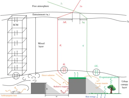
Figure 1.Schematics of coupled SLUCM–SCM framework: land surface processes are parameterized by a single layer urban canopy model; atmospheric processes under convective condition are parameterized by a single column model.
The schematic of the coupled SLUCM–SCM framework is shown in Fig. 1, which captures three vertical layers. The lowest level is the surface layer, which is considered as the constant flux layer and consists of 10 % of the entire CBL with the built terrain located at the bottom. The middle level is a convective mixed layer, where distributions of tempera-ture and humidity are determined by buoyant plumes arising from the surface layer and atmospheric turbulence. The top level is an entrainment zone with a temperature inversion, which inhibits upward mixing and confines subjacent air and pollution in the CBL. Temperature and humidity profiles in the entire vertical column are regulated by heat and moisture fluxes exchanged across the interfaces of two adjacent layers. At the bottom of numerical framework, the urban canopy layer is parameterized by a SLUCM, which is also adopted in the latest version of Weather Research and Forecast (WRF) model (v3.7.1) (Yang et al., 2015). This new SLUCM fea-tures enhanced urban hydrological processes coupled with the urban energy balance model, which enables a more re-alistic representation of the transport of energy and water over built terrains. The energy balance equation for the ur-ban canopy layer is given by
Rn+AF=Hu+LEu+G0, (1)
whereRnis the net radiation;AF is the anthropogenic heat
fluxes;Huand LEuare the turbulent sensible and latent heat
fluxes arising from the entire urban canopy layer, respec-tively; G0 is the conductive heat flux aggregated over
ur-ban sub-facets (i.e., roof, wall, and ground), where the actual
thickness and thermal mass of these solid media have been taken into account. Note that the thermal energy involved in advection, radiative flux divergence, and canyon air temper-ature variation is considered small when compared with the energy stored in urban surfaces (Nunez and Oke, 1977). It is noteworthy that, in reality, the surface energy balance is usu-ally not closed in field experiments but rather an energy resid-ual is found (see Foken, 2008, for a comprehensive review on this subject). In addition, a posteriori analysis of surface en-ergy budgets found that only 1 % of the residual variance can be attributed to advection and is not statistically significant (Higgins, 2012).
The turbulent sensible and latent heat fluxes arising from the urban area (Huand LEu)are the areal average of those
from roofs (HRand LER)and the street canyon (Hcan and
LEcan)(Wang et al., 2013):
Hu=r
NR
X
k=1
fR,kHR,k+wHcan, (2)
LEu=r
NR
X
k=1
fR,kLER,k+wLEcan. (3)
Hcan= 2h w NW X k=1
fW,kHW,k+ NG
X
k=1
fG,kHG,k, (4)
LEcan=
2h w
NW
X
k=1
fW,kLEW,k+ NG
X
k=1
fG,kLEG,k. (5)
NR,NW, andNGare the number of sub-facet types of roofs,
walls and ground (road), respectively; fR,fW, andfG are
the fraction of sub-facet types of roofs, walls, and ground, respectively; r=R/(R+W ), w=W/(R+W ), and h= H /(R+W ) are the normalized roof width, canyon width, and building height, respectively, withR,W, andHas phys-ical dimensions. By assuming that surface layer is a constant flux layer, the turbulent fluxes at the top of surface layer (viz. the “constant” flux layer occupying the bottom∼10 % of the CBL; see Stull, 1988) are the same with those arising from the urban canopy (Huand LEu).
To resolve the overlying atmospheric boundary layer, a modified version of the Yonsei University (YSU) boundary layer scheme commonly used in the WRF model (Hong et al., 2006; Noh et al., 2003) was applied by incorporating an analytical prognostic formula (Ouwersloot and Vilà-Guerau de Arellano, 2013) rather than a diagnostic formula related with Richardson number (Hong et al., 2006) for determining the boundary layer height. In the mixed layer, the governing equation for mean profiles of virtual potential temperature and specific humidity due to boundary layer turbulence in SCM is given by (Troen and Mahrt, 1986)
∂θv
∂t =
∂ ∂z(−w
′θ′
v), (6)
∂q ∂t =
∂ ∂z(−w
′q′), (7)
whereθvis the virtual potential temperature;qis the specific
humidity;wis the vertical wind speed; andw′X′withX= θvorq is the vertical kinematic eddy flux, with the overbar
denoting the ensemble average. The vertical kinematic eddy heat and moisture flux at the lower boundary of the mixed layer is given by
w′θ′
s=
Hs
ρacp
, (8)
w′q′
s=
LEs
ρaLv
, (9)
where subscript s denotes the atmospheric surface layer,θis the potential temperature,ρais the density of the air,cpis the specific heat of air at constant pressure, andLvis the latent
heat of vaporization of water. From the definition of virtual potential temperature, we have
w′θv′s=0.61θ w′q′s+(1+0.61q) w′θ′s. (10)
The upper boundary condition is at the height of CBL (zh),
which appears as a mixing height scale in turbulence closure
schemes in climate and weather prediction models and acts as an impenetrable lid for pollutants released at the surface (Zilitinkevich and Baklanov, 2002). The height of CBL is de-termined as (Ouwersloot and Vilà-Guerau de Arellano, 2013) zh=
z2h0+(2+4we) γθv
1θv,0z
1+we
we
h0 −
w
e
1+2we
γθvz
1+2we
we h0 ˆ z− 1 we
h −z
−w1 e h0
+
2+4we
γθv
Zt
t0
w′θv′
sdt
1/2
, (11)
wherezh0 is the initial CBL height, we is the entrainment
rate at the inversion,γθv is the lapse rate in the free
atmo-sphere,1θsis the potential temperature difference across the
inversion, andzˆhis a correction term given by
ˆ zh=
z2h0+
2+4we
γθv
Zt
t0
w′θv′sdt
1/2
. (12)
The turbulent kinematic heat and moisture fluxes at the upper boundary of mixed layer (Hong et al., 2006; Kim et al., 2006) are
w′θ′
v
zh
= −0.15
θ
v
g
w3m/zh, (13)
w′q′
zh
≈0, (14)
wherewmis the velocity scale for entrainment (wm3 =w∗3+
5u3∗), which can be derived from the mixed layer velocity
scale w∗ and surface friction velocity scale u∗, and w∗ is
parameterized by
w∗=
hg
θ
w′θ′ szh
i1/3
, (15)
accounting for the surface heat fluxw′θ′
sat lower
bound-ary of mixed layer and CBL heightzh. Equation (13) implies
that the entrainment heat flux is closely related to the surface layer states. In large eddy simulations, the heat flux at the entrainment/inversion is usually estimated by
w′θv′
zh
w′θv′
s
= −AR, (16)
with AR=0.15 typically (Hong et al., 2006; Kim et al.,
2006; Noh et al., 2003). The upward heat flux from land sur-face and the downward heat flux at the inversion layer both enhance turbulent mixing in the mixed layer.
en-trainment effect can be parameterized as (Noh et al., 2003)
−w′θv′ =Kh
∂θ
v
∂z −γh
−w′θv′
h
z
zh
3
, (17)
−w′q′=K
h
∂q
∂z−γq
−w′q′
h
z
zh
3
, (18)
where Kh is turbulent diffusivity which is assumed to be
identical for heat and moisture transport;zis the vertical dis-tance from surface; γh andγq are non-local mixing terms (Noh et al., 2003; Troen and Mahrt, 1986), given by
γh=C
w′θ′
s
wszh
, (19)
γq=C
w′q′
s
wszh
, (20)
whereC is a coefficient of proportionality, often set as 6.5 according to Troen and Mahrt (1986), andws is the
veloc-ity scale for the entire CBL. With prescribed initial states (i.e., profiles of θv and q) and boundary conditions given
by Eqs. (8)–(14), we can readily estimate the time evolution and vertical profiles of temperature and humidity in the CBL based on the above physical parameterization schemes. 2.2 Model evaluation
To evaluate the coupled SLUCM–SCM framework outlined in Sect. 2.1, experiment data of temperature and humid-ity profiles were obtained from NOAA/ESRL radiosonde database (http://esrl.noaa.gov/raobs/) for two typical con-vective days, i.e., 2 July and 9 July 2013 at Phoenix site (33.45◦N, 111.95◦W), Arizona. All atmospheric data in the ESRL Radiosonde database were subjected to gross error and hydrostatic consistency checks according to Schwartz and Govett (1992). The coupled modeling framework was driven by surface meteorological variables measured by a network of wireless meteorological stations (33.44◦N, 111.92◦W) in the closest vicinity of the footprint area of the radiosonde site (see Song and Wang, 2015b, for details). The comparison of the simulated and observed profiles of virtual potential tem-perature and specific humidity is shown in Fig. 2 for the two days at 16:44 and 16:37 LT (local time), respectively. Major difference between the observed and modeled profiles occurs in the surface layer. This is mainly due to that the SCM in the modeling framework uses Monin–Obukhov similarity theory (MOST) for parameterizing the surface layer profiles, as well as the mismatch in source areas. MOST assumes homogene-ity of turbulence and surface conditions, which is rarely sat-isfied for the atmospheric boundary layer over a built terrain. Also note that the integrated SLUCM–SCM framework can be readily tested on the WRF platform in an online setting, i.e., by coupling with other dynamic modules (e.g., radiation, Noah land surface model for natural terrains). Here we
fo-cused on the sensitivity of the offline (stand-alone) SLUCM– SCM framework to exclude the physical and numerical per-turbation (e.g., model stability) that could potential arouse from the online testing with coupling to mesoscale dynamics (e.g., regional advection, synoptic influence).
2.3 Subset simulation
In urban climate modeling, the capability of assessing critical responses of atmospheric processes to urban land use/land cover change is of paramount significance for assessment of climatic extremes. The SLUCM–SCM framework cou-pling urban land surface processes and CBL dynamics in-volves a large number of input parameters, which leads to high dimensionality of input space for the following statis-tical analysis. Hence we adopt subset simulation (Au and Beck, 2001; Au and Wang, 2014) for subsequent sensitivity study, which is efficient in simulating rare (very small prob-ability) events and robust for high dimensionality. Instead of simulating rare events as in direct MCS method with ex-pensive computational cost, subset simulation breaks down extreme events with small exceedance probability into a se-quence of more frequent events by introducing intermediate exceedance events. The targeted small exceedance probabil-ity is then expressed as a product of larger conditional proba-bilities of each intermediate event. In addition, MCMC tech-nique is adopted based on effective accept/reject rules in sub-set simulations to improve computational efficiency.
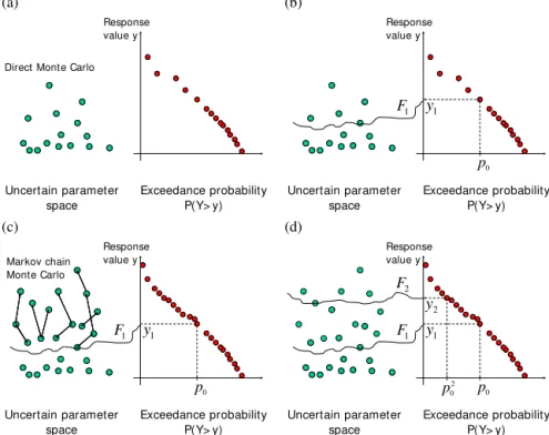
As illustrated in Fig. 3, the sampling technique employed in the subset simulation proceeds as follows: in level 0 (ini-tial state), the unconditional samples of uncertain parameters follow a prescribed probability distribution function (PDF) (Fig. 3a). Conditional samples in level 1 are defined using a given intermediate conditional probabilityp0(e.g.,p0=0.1
stands for 10 % of the level 0 samples will be selected as conditional samples) (Fig. 3b). These samples are then gen-erated by MCMC procedure using importance sampling at the exceedance probabilityP (Y > y1)=p0(Y is a critical
response of model andy1is a threshold value) (Fig. 3c).
Sub-sequent conditional sampling are conducted by MCMC with the intermediate exceedance probability target, i.e.,P (Y > yi)=p0i (i=1, 2, 3, . . . denoting conditional levels) until
simulations reach the final target withpf =pN0, wherepf is the target probability of a rare event andN the total num-ber of conditional levels (Fig. 3d). Using this method, a rare event, e.g., with target exceedance probability ofpf =10−4 (i.e., the probability of occurrence is less than 1 in 10 000), can be effectively broken down into four different sampling (one unconditional MCS and three subsequent conditional MCMC) levels; each samples a moderate conditional prob-ability ofp0=0.1.
θ
v(K)
z
(m
)
310 315 320 325
0 500 1000 1500 2000 2500 3000 3500 (b)
q(kg kg-1
)
z
(m
)
0 0.005 0.01 0.015 0.02
0 500 1000 1500 2000 2500 3000 3500
q(kg kg-1
)
z
(m
)
0 0.005 0.01 0.015 0.02
0 500 1000 1500 2000 2500 3000 3500
θ
v(K)
z
(m
)
305 310 315 320 325 330 335
0 500 1000 1500 2000 2500 3000 3500
Simulated Measured (a)
Figure 2.Comparison of simulated and measured atmospheric profiles of virtual potential temperatureθvand specific humidityqfor two
time points, i.e.,(a)16:44 LT on 2 July 2013 and(b)16:37 LT on 9 July 2013 at NOAA-ESRL Phoenix site.
(a) (b)
(c) (d)
Response value y
Exceedance probability P(Y> y) Uncertain parameter
space
Direct Monte Carlo
1 F
0 p
Uncertain parameter space
Exceedance probability P(Y> y)
Response value y
1
y
Markov chain Monte Carlo
1 F
0 p
Uncertain parameter space
Exceedance probability P(Y> y)
Response value y
1
y F1
0 p 2 0 p 2 F
Uncertain parameter space
Exceedance probability P(Y> y)
Response value y
1
y
2
y
Figure 3.Schematic of subset simulation procedure:(a)level 0 (initial phase) sampling by direct MCS,(b)determination of level 1 samples
F1given conditional exceedance probabilityp0,(c)populating conditional samples in level 1 by MCMC procedure, and(d)forwarding
Exceedance probability
C
o
ef
fi
cien
t
o
f
v
ar
iatio
n
10-4
10-3
10-2
10-1
100
0.0 0.5 1.0 1.5 2.0 2.5
Subset simulation MCS
NT= 500 NT= 1850
NT= 1400
NT= 950
Figure 4.Comparison of the coefficient of variation of exceedance probability in subset simulation and direct MCS.
of subset simulation as a function of exceedance probabil-ity is shown in Fig. 4, where c.o.v. of direct MCS is also shown for comparison. Estimate of c.o.v. of direct MCS can be analytically formulated as [(1−pi)/(piNT)]1/2 (Au and Beck, 2001), wherepi is the exceedance probability andNT the number of samples at corresponding MCMC leveli. It is clear that the c.o.v. of subset simulation is significantly smaller than that of direct MCS, especially at the higher MCMC level (smaller probability), indicating less statistical error for exceedance probability estimates using subset sim-ulation.
3 Results of sensitivity analysis
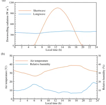
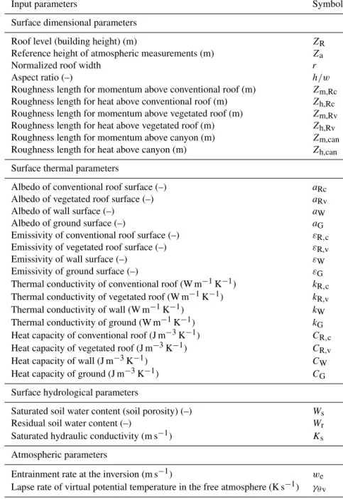
In this section, we apply subset simulation to analyze the sen-sitivity of the coupled SLUCM–SCM to different input pa-rameters. The meteorological forcing in the surface layer was prescribed using field measurements of an eddy covariance tower on a clear day (14 June 2012) provided by the Cen-tral Arizona–Phoenix Long-Term Ecological Research (CAP LTER) project (Chow et al., 2014). The inputs of diurnal air temperature, relative humidity, and downwelling shortwave and longwave radiation are plotted in Fig. 5, with the day-time from 06:00 to 19:30 (local day-time) for the development of CBL. With the prescribed meteorological forcing, the surface sensible and latent heat fluxes are predicted by the SLUCM, which then in turn drive the SCM to estimate temperature and humidity profiles in the mixed layer. The input param-eters of SLUCM–SCM (including surface dimensional and hydrothermal parameters for the SLUCM and atmospheric parameters for the SCM) are presented in Table 1. Note that the initial soil water content for green roofs in the SLUCM is set as 90 % saturated for the subsequent 13.5 h of simulation after the beginning of CBL development such that the evap-orative power of green roofs is not constrained by soil water
Local time (h)
D
o
w
n
w
ellin
g
rad
iatio
n
(W
m
-2)
0 2 4 6 8 10 12 14 16 18 20 22 24
0 300 600 900 1200
Shortwave Longwave (a)
Local time (h)
A
ir
te
m
pe
ra
tu
re
(
oC)
R
elativ
e
h
u
mid
ity
(%
)
0 2 4 6 8 10 12 14 16 18 20 22 24
0 10 20 30 40 50
0 10 20 30 40 50
Air temperature Relative humidity (b)
Figure 5.The diurnal surface atmospheric forcing of 14 June 2012
(a clear day) in Phoenix, AZ:(a)downwelling shortwave and
long-wave radiation and(b)air temperature and relative humidity. The
daytime data between starting point (06:00 LT) and ending point (19:30 LT) are used to drive the SLUCM–SCM under convective condition.
bound-Table 1.Input parameters of the coupled SLUCM–SCM numerical framework.
Input parameters Symbol
Surface dimensional parameters
Roof level (building height) (m) ZR
Reference height of atmospheric measurements (m) Za
Normalized roof width r
Aspect ratio (–) h/w
Roughness length for momentum above conventional roof (m) Zm,Rc
Roughness length for heat above conventional roof (m) Zh,Rc
Roughness length for momentum above vegetated roof (m) Zm,Rv
Roughness length for heat above vegetated roof (m) Zh,Rv
Roughness length for momentum above canyon (m) Zm,can
Roughness length for heat above canyon (m) Zh,can
Surface thermal parameters
Albedo of conventional roof surface (–) aRc
Albedo of vegetated roof surface (–) aRv
Albedo of wall surface (–) aW
Albedo of ground surface (–) aG
Emissivity of conventional roof surface (–) εR,c
Emissivity of vegetated roof surface (–) εR,v
Emissivity of wall surface (–) εW
Emissivity of ground surface (–) εG
Thermal conductivity of conventional roof (W m−1K−1) kR,c
Thermal conductivity of vegetated roof (W m−1K−1) kR,v
Thermal conductivity of wall (W m−1K−1) kW
Thermal conductivity of ground (W m−1K−1) kG
Heat capacity of conventional roof (J m−3K−1) CR,c
Heat capacity of vegetated roof (J m−3K−1) CR,v
Heat capacity of wall (J m−3K−1) CW
Heat capacity of ground (J m−3K−1) CG
Surface hydrological parameters
Saturated soil water content (soil porosity) (–) Ws
Residual soil water content (–) Wr
Saturated hydraulic conductivity (m s−1) Ks
Atmospheric parameters
Entrainment rate at the inversion (m s−1) we
Lapse rate of virtual potential temperature in the free atmosphere (K s−1) γθv
ary conditions according to Ouwersloot and Vilà-Guerau de Arellano (2013).
3.1 Critical model responses
Three atmospheric variables, i.e., the critical CBL height (zh), the mean virtual potential temperature (θv), and the
mean specific humidity (q)in the mixed layer, are selected as model responses to assess the impact of urban land sur-face characteristics on the overlying atmosphere. “Critical” means that extreme responses of these model outputs (with small exceedance probability, or equivalently as “climatic extremes”) are simulated using MCMC procedure. This is
particularly relevant when urban planning is concerned with mitigation strategies of extreme events associated with future land use and climatic changes. For each monitored output, we simulate three different cases with the fraction of green roof vegetation of 0, 0.5, and 1.0, respectively. Note that we do not include vegetation on ground (though the model is capable of), so roof vegetation is the only moisture source. This model set-up allows us to analyze exclusively the effec-tiveness of green roofs, one of the urban environmental miti-gation strategies of particular interest to researchers and city planners. For all three cases, three conditional levels are used with a conditional probability ofp0=0.1, which is
Table 2.Summary of statistics of uncertain parameters used in the sensitivity study.
Type Parameter Unit PDF Min Max Mean SD
Surface thermal parameters aRv – Normal 0.05 0.6 0.18 0.045
CRv MJ m−3K−1 Normal 0.1 2 0.72 0.18
kRv W m−1K−1 Normal 0.15 4 0.85 0.213
aRc – Normal 0 1 0.15 0.0375
CRc MJ m−3K−1 Normal 0.1 4 1.52 0.38
kRc W m−1K−1 Normal 0.2 3 1.2 0.3
Surface hydrological parameters Ws – Normal 0.3 0.6 0.44 0.074
Wr – Normal 0.04 0.2 0.074 0.025
Ks m s−1 Normal 0.1 100 1.7 0.43
Surface dimensional parameters r – Uniform 0.3 0.8 – –
h/w – Uniform 0.25 8 – –
Zm,Rc mm Uniform 0.1 5 – –
Zm,Rv mm Uniform 10 200 – –
Atmospheric parameters we m s−1 Uniform 0.1 0.3 – –
γθv K km−1 Uniform 3 7 – –
and 10−3for MCMC levels 1, 2, and 3, respectively. In to-tal, 270 simulations were run (30 independent simulations per case for 9 cases) with 1450 realizations of the set of 15 uncertain parameters in each run to ensure the simulation re-sults are statistically significant.
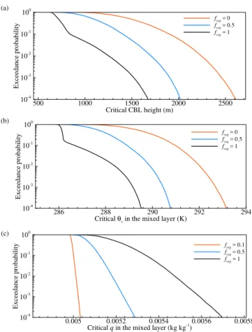
Plots of exceedance probabilities versus various model re-sponses averaged over 30 simulations are presented in Fig. 6. The variations of critical model outputs with three different green roof fractions indicate the sensitivity of roof greening degrees on CBL dynamics. In Fig. 6a and b, we monitored CBL height and virtual potential temperature of mixed layer under three conditions of green roof fractions (i.e.,fveg=0,
0.5, and 1). In general, larger green roof fractions lead to lowerzhand smallerθv. This is expected since urban
land-scapes with larger fraction of vegetation distribute solar en-ergy into more latent heat and less sensible heat, due to evap-orative cooling. Less sensible heat and reduced surface tem-perature both lead to reduced CBL height and virtual poten-tial temperature.
It is also noteworthy that there exist log concavities for the exceedance probabilities of both critical zh andθvwith
fveg=1 (100 % roof greening). The occurrence of log
con-cavities is related to energy balance in the street canyon where nonlinear effect of canyon aspect ratioh/w was ob-served (Song and Wang, 2015a). Detailed explanations of as-pect ratio effects will be described in Sect. 4.1. In Fig. 6c, we monitored specific humidity of mixed layer under three con-ditions of green roof fractions (i.e.,fveg=0.1, 0.5, and 1). As
roof is set as the only moisture source, urban land surface is completely dry withfveg=0 and resulted in no moisture in
the atmosphere in the absence of horizontal advection. Larger green roof fraction tends to produce higherqin the overlying CBL. In contrast tozhandθv, exceedance probability
distri-Critical CBL height (m)
Ex
ceed
an
ce
p
ro
b
ab
ility
500 1000 1500 2000 2500
10-4
10-3
10-2
10-1 100
fveg= 0
fveg= 0.5
fveg= 1 (a)
Criticalθ
vin the mixed layer (K)
Ex
ceed
an
ce
p
ro
b
ab
ility
286 288 290 292 294
10-4 10-3
10-2 10-1
100
fveg= 0
fveg= 0.5
fveg= 1 (b)
Criticalqin the mixed layer (kg kg-1
)
Ex
ceed
an
ce
p
ro
b
ab
ility
0.005 0.0052 0.0054 0.0056 0.0058
10-4
10-3 10-2
10-1
100
fveg= 0.1
fveg= 0.5
fveg= 1 (c)
Figure 6.Estimates of exceedance probabilities for model outputs
of critical(a)CBL height,(b) virtual potential temperature, and
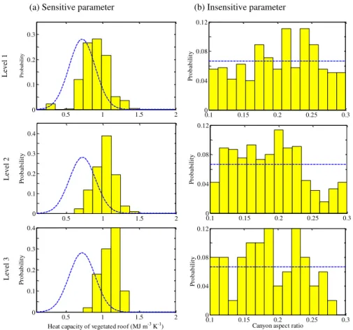
bution of critical response ofqdoes not exhibit log concavity because the moisture source is purely from roofs and canyon aspect ratio and building density have no contribution. 3.2 Statistical quantification of model sensitivity In general, for an uncertain parameter, the deviation be-tween the distribution of MCMC-generated conditional sam-ples (in levels 1, 2, and 3) and the initial prescribed distri-bution sampled using direct MCS (level 0) indicates the sig-nificance of parameter sensitivity with respect to the corre-sponding model output. Figure 7 shows the comparison be-tween conditional distribution (histograms) and initial dis-tribution (dashed line) for two sample parameters, i.e., heat capacity of green roofCRvand canyon aspect ratioh/w,
re-spectively, for a typical simulation withfveg=1.0 and
criti-calq as model output. It is clear that the critical response of q is more sensitive toCRvwith noticeable deviation of
sam-ple distribution at each conditional level (Fig. 7a), whileh/w is relatively insignificant in influencingq with small devia-tion of sample distribudevia-tion (Fig. 7b). The result is physical as variation ofCRvaffects roof surface energy balance, which in
turn influences the humidity profile in the CBL through sur-face moisture flux. On the contrary, since green roofs are the only moisture source in our setting, alteringh/whas negligi-ble effect on the atmospheric moisture for the street canyon with no vegetation on ground or wall.
To better quantify the parameter sensitivity, a percentage sensitivity index (PSI) (Wang et al., 2011a) is adopted here to measure the model sensitivity to an uncertain parameter Xby calculating the average deviation of conditional sample means to that of the original PDF:
PSI[X] = 1 N
N X
i=1
EX|Y > yi
−E[X]
E[X] , (21)
wherei is the conditional (MCMC) level index,N=3 the total conditional levels,E[X] the statistical mean (expected value) of the original unconditional distribution in level 0 (as in Table 2),E[X|Y > yi] the mean value ofXat conditional leveli,Y the value of monitored model response, andyi the threshold values at exceedance probability of each intermedi-ate leveli. The magnitude of PSI quantifies the significance of sensitivity, while the sign of PSI indicates the correlation between monitored outputYand input parameterX, i.e., pos-itive PSI means increasingXwill lead to an increase of out-put Y and negative PSI means increasingX will lead to a decreasedY.
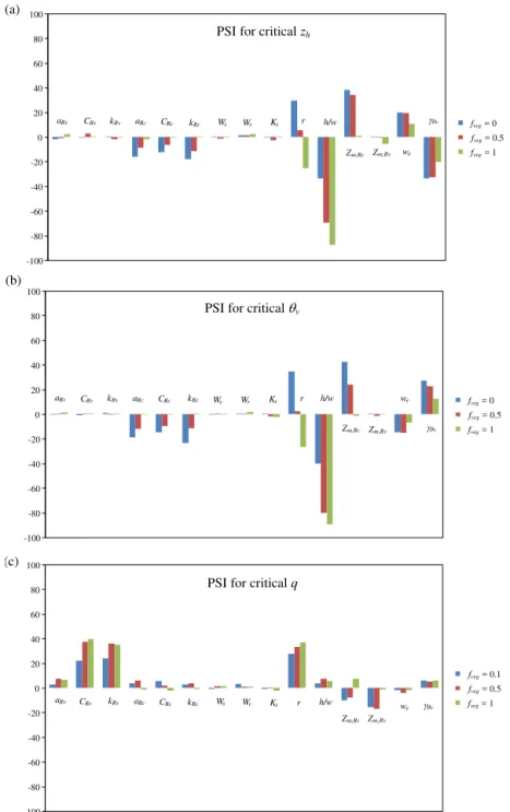
PSI values of all uncertain parameters for three different monitored outputs, i.e., zh, θv, andq, with different green
roof fractions are shown in Fig. 8. As shown in Fig. 8a and b, bothzhandθvare highly sensitive to surface dimensional
parameters, including normalized roof width r, canyon as-pect ratioh/w, and roughness length of momentum for con-ventional roofs Zm,Rc. Note that r is positively correlated
with criticalzhandθvfor conventional roofs while the
cor-relation is negative for green roofs. Both criticalzhandθv
are negatively correlated withh/wand positively correlated withZm,Rc. Moderate sensitivity of criticalzhandθvis found
with respect to thermal parameters of conventional roofs in-cluding albedoaRc, heat capacityCRc, and thermal
conduc-tivitykRc. Also note that there are opposite correlations for
atmospheric parameterswe andγθv:zh is positively
corre-lated withweand negatively correlated withγθv, but the
cor-relations are opposite for model output of criticalθv. From
Fig. 8c, mixed layerq is highly sensitive to r and thermal properties of green roofs and moderately sensitive toZm,Rv.
Physical mechanisms governing the model sensitivity and its implications to urban planning are discussed below.
4 Discussion
The UHI effect has attracted significant effort are even heated debate from urban climate researchers and city planners. UHI is characterized by elevated temperature in built environ-ments compared to surrounding rural areas (Oke, 1982). Ma-jor contributors of UHI include (a) excess storage of thermal energy due to radiative trapping by street canyon and ther-mal properties of pavement materials, (b) reduced vegetation cover and evaporative cooling, and (c) the release of anthro-pogenic heat, moisture, and greenhouse gases (Santamouris, 2014; Sun et al., 2013a). Correspondingly, there are several popular UHI mitigation strategies, including (1) changing canyon geometry (characterized by aspect ratio and rough-ness lengths) to alter the energy distribution through radiative shading and trapping; (2) changing thermal properties, such as installing cool roofs or cool pavements to reflect more so-lar radiation by increasing surface albedo; (3) adding green spaces, such as green roofs to increase evapotranspiration in urban area. We will discuss the effects of these UHI miti-gation strategies on the overlying atmosphere based on the sensitivity study and its implication to urban planning. 4.1 Impact of urban morphology
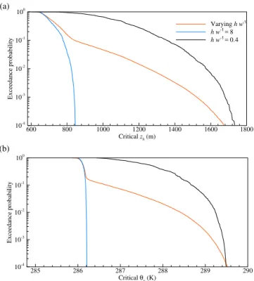
Building geometry and density in an urban area have a sig-nificant impact on the partitioning and redistribution of solar energy in the surface layer, which in turn modulate the energy transport processes in the overlying atmosphere. The canyon aspect ratioh/wis a typical indicator of building geometry and density in urban planning (Ali-Toudert and Mayer, 2006; Krüger et al., 2011; Theeuwes et al., 2013). Lowh/wsignals low building (smallh)or sparse building density (largew), while high h/w indicates high building (large h)or inten-sive building density (smallw). With variable aspect ratio ranging from 0.25 to 8, log concavity is found in the ex-ceedance probability estimates for criticalzh andθv in the
case offveg=1.0 as shown in Fig. 5a and b. This log
L
eve
l
1
L
eve
l
2
0.5 1 1.5 2
0 0.1 0.2 0.3
P
roba
bi
li
ty
0.5 1 1.5 2
0 0.1 0.2 0.3 0.4
P
ro
b
a
b
il
it
y
L
eve
l
3
0.5 1 1.5 2
0 0.1 0.2 0.3 0.4
Heat capacity of vegetated roof (MJ m-3 K-1)
P
ro
b
a
b
il
it
y
0.1 0.15 0.2 0.25 0.3
0 0.04 0.08 0.12
P
ro
b
a
b
il
it
y
0.1 0.15 0.2 0.25 0.3
0 0.04 0.08 0.12
P
ro
b
a
b
il
it
y
0.1 0.15 0.2 0.25 0.3
0 0.04 0.08 0.12
Canyon aspect ratio
P
ro
b
a
b
il
it
y
(a) Sensitive parameter (b) Insensitive parameter
Figure 7.Histogram of conditional samples at different conditional levels for(a)a sensitive parameter and(b)an insensitive parameter for
a typical simulation withfveg=1.0 and criticalqas model output.
aspect ratio on CBL height and virtual potential temperature, due to two counteracting processes, viz. shading effect and radiative trapping effect in the street canyon, as investigated by Song and Wang (2015a). To further test the nonlinear ef-fect ofh/won CBL dynamics, we set the canyon aspect ratio constant, and the log concavity disappears as shown in Fig. 9. The log concavity of variable h/w demarks the switching from smallh/wcase to highh/w case with a nonlinear in-teraction between radiative shading and trapping effects. In addition, at mesoscale atmospheric modeling, the canyon as-pect ratio is closely related to the surface roughness of a built terrain, which in turn modulates the surface aerodynamic re-sistance under convective condition and further complicate the nonlinear effect.
4.2 Impact of thermal properties
As shown in Fig. 8, CBL states (zh,θv, andq)are moderately
sensitive to surface thermal properties. Specifically,aRc,CRc,
and kRc of conventional roofs are important parameters in
modulatingzhandθv, whereasq is sensitive toCRvandkRv
of green roofs. Higher albedo causes more solar energy be-ing reflected and less sensible heat arisbe-ing from roofs, lead-ing to smallerzhandθv. Moderate model sensitivity toaRc
demonstrates that implementation of white/cool roofs with
higher reflectivity is an effective way in reducing environ-mental temperature not only in the urban surface layer but also in the overlying mixed layer.
(a)
-100 -80 -60 -40 -20 0 20 40 60 80 100
PSI for critical zh
fveg = 0
fveg = 0.5
fveg = 1 aRv CRv kRv aRc CRc kRc Ws Wr Ks r h/w
Zm,Rc Zm,Rv we gqv
(b)
-100 -80 -60 -40 -20 0 20 40 60 80 100
PSI for critical qv
fveg = 0
fveg = 0.5
fveg = 1 aRv CRv kRv aRc CRc kRc Ws Wr Ks r h/w
Zm,Rc Zm,Rv we
gqv
-100 -80 -60 -40 -20 0 20 40 60 80 100
PSI for critical q
fveg = 0.1
fveg = 0.5
fveg = 1 aRv CRv kRv aRc CRc kRc Ws Wr Ks r h/w
Zm,Rc Zm,Rv we gqv (c)
Figure 8.PSI values for model outputs of critical(a)zh,(b)mixed layerθv, and(c)mixed layerq, with different green roof fractions.
q via evaporative cooling. Nevertheless, we emphasize here that what the PSI values can reveal is as good as that the coupled SLUCM–SCM framework can capture. The actual physics of urban land–atmosphere interactions involves more complicated land surface and atmospheric processes of heat and water transport in the integrated soil–atmosphere sys-tem due to complexity of surface energy partitioning (Yang and Wang, 2014a). For example, the existence of phase lags among land surface temperatures and energy budgets, due to subsurface heat transport with pore water advection, can
lead to complex hysteresis loops (Sun et al., 2013b; Wang, 2014) that are not adequately captured by the current numer-ical framework.
4.3 Impact of green roofs
Criticalzh(m)
Ex
ceed
an
ce
p
ro
b
ab
ility
600 800 1000 1200 1400 1600 1800
10-4
10-3
10-2
10-1
100
Varyinghw hw = 8
hw = 0.4 (a)
Criticalθ
v(K)
Ex
ceed
an
ce
p
ro
b
ab
ility
285 286 287 288 289 290
10-4
10-3
10-2
10-1
100
(b)
-1 -1 -1
Figure 9.Illustration of the nonlinear effect of aspect ratioh/won
critical model responses of(a)zhand(b)θvof the CBL
(1) thermal parameters, i.e.,aRv,CRv, andkRv; (2)
hydrolog-ical parameters, i.e., saturated soil water contentWs, residual
soil water contentWr, and saturated hydraulic conductivity
Ks; (3) roof widthr; and (4) green roof fractionfveg.
Humid-ity in the CBL is moderately sensitive to green roof thermal properties with a positive correlation, as discussed above. In addition, all hydrological parameters are relatively insensi-tive as shown in Fig. 8. This is plausibly due to the initial soil moisture condition (90 % saturated), which is realistic provided green roofs are carefully maintained with constant irrigation. The assumption is also relevant in this study for more “manageable” urban surface characteristics for urban planning purpose. Sensitivity analysis of boundary layer dy-namics related to soil water and hydrological properties of other urban vegetation (such as urban lawns, urban agricul-ture), however, require further investigation (Cuenca et al., 1996; Song and Wang, 2015b).
In contrast, CBL dynamics are very sensitive to green roof width and areal fractions, as they determine the area of green roof in a built environment, which in turn strongly influence the soil water availability for evaporation. It is shown that larger green roof widthrand fractionfveglead to lowerzh,
smaller θv, and higher q in the mixed layer as a result of
evaporative cooling by green roofs. This result is expected and clearly indicates the effectiveness of green roofs in reg-ulating atmospheric dynamics above an urban area. To fur-ther test the effectiveness of green roofs, we monitored the same set of model outputs, viz.zh,θv, andq, withfveg
rang-ing from 0 % to 100 % with an increment of 10 %. Thresh-old values at three conditional sampling levels are plotted in Fig. 10, i.e.,yi for i=1, 2, and 3, with corresponding ex-ceedance probability of 10−1, 10−2, and 10−3, respectively. For all output variables at different conditional levels, the re-sults can be well fitted using linear relations with high R2 values:zhandθvdecrease linearly with the green roof
frac-tion, whileqincreases linearly withfveg. As far as UHI
mit-igation is concerned, the mean mixed layer temperature can be reduced by 3–4 K in either a more probable (level 1) or a more extreme (level 3) case with an increase of green roof fraction from 0 to 100 %. It is noteworthy that, in this study, the supply of soil water content to green roof systems is as-sumed to be ample (e.g., via urban irrigation). In an arid en-vironment such as Phoenix, especially during drought, the trade-off between water (for irrigation) and energy (cooling load) needs to be carefully measured by city planners. 4.4 Impact of roughness lengths
Roughness lengths of momentum and heat transfer are im-portant land surface characteristics that regulate the aero-dynamic resistance related to turbulent transport of mass, momentum and energy in the surface layer (Grimmond and Oke, 1999). Specifically, aerodynamic resistance is a func-tion of roughness length based on MOST (Mascart et al., 1995; Wang et al., 2013). In this study, we set the rough-ness lengths of momentum at the roof level as uncertain pa-rameters for both conventional and green roofs. The rough-ness lengths of heat transfer follow a simple parameterization thatZh=Zm/10 (Mascart et al., 1995). From Fig. 8, both
zh andθv in the mixed layer are highly sensitive toZm,Rc,
whileZm,Rv of green roofs plays an important role in
reg-ulatingq. As indicated in Table 3, when criticalzhis
moni-tored, PSI value ofZm,Rcis 38.53 % forfveg=0 and 34.42 %
for fveg=0.5; for critical θv, PSI of Zm,Rc is 42.58 % for
fveg=0 and 24.38 % forfveg=0.5. These high PSI values
indicate a strong correlation between aerodynamic resistance of turbulent transfer and the CBL dynamics. This implies that altering roughness lengths of roofs (i.e., changing dif-ferent vegetation types with difdif-ferent height over green roof and changing different materials over conventional roof) is an effective way to influence energy transport from surface to the overlying CBL without fundamental changes to the ur-ban morphology or geometry in the street canyon.
In addition to urban landscape characteristics, the coupled SLUCM–SCM numerical framework also involves physi-cal parameterizations at the top of CBL, i.e., in the inver-sion layer. The uncertainties of two atmospheric parameters, namely the entrainment ratewe and the lapse rate of
vir-tual potential temperatureγθv are tested. From Fig. 7a,zh
increases withwe and decreases withγθv, as expected
ac-cording to Eq. (11). From Fig. 8b, impacts ofweandγθvon
critical mixed layerθvare opposite. This is because largerwe
zh= -10.83 fveg+ 1932 R² = 0.992 zh= -10.621 fveg+ 2251
R² = 0.989 zh= -9.71 fveg+ 2419
R² = 0.985
0 500 1000 1500 2000 2500 3000
0 10 20 30 40 50 60 70 80 90 100
C
ritica
l
zh
(m)
Green roof fraction, fveg(%)
Level 1 - MCMC Level 2 - MCMC Level 3 - MCMC
qv= -0.043 fveg+ 291 R² = 0.996 qv= -0.0367 fveg+ 292
R² = 0.984 qv= -0.034 fveg+ 292
R² = 0.971
286 288 290 292 294
0 10 20 30 40 50 60 70 80 90 100
C
ritica
l
qv
(K
)
Green roof fraction, fveg(%)
q= 4E-06 fveg+ 0.005 R² = 0.984 q= 5E-06 fveg+ 0.005
R² = 0.990 q= 6E-06 fveg+ 0.005
R² = 0.987
4.9E-03 5.1E-03 5.3E-03 5.5E-03 5.7E-03
0 10 20 30 40 50 60 70 80 90 100
C
ritica
l
q
(kg
kg
-1)
Green roof fraction, fveg(%)
(a)
(b)
(c)
Figure 10.Threshold values at different conditional levels as functions of green roof fractions for critical(a)zh,(b)mixed layerθv, and
(c)mixed layerq. MCMC levels 1, 2, and 3 correspond to exceedance probabilities of 10−1, 10−2, and 10−3, respectively.
further cause smaller non-local mixing effects according to Eqs. (19) and (20), leading to a decrease ofθvin the mixed
layer.
5 Concluding remarks
In this study, we use an advanced Monte Carlo method to quantify the sensitivity of atmospheric boundary layer dy-namics to urban land surface characteristics based on a
shading in the street canyon. Specifically, rooftop planning strategies strongly modulate CBL dynamics. Besides, chang-ing roughness lengths or thermal properties on rooftops (e.g., by planting different species of vegetation for green roofs or using porous pavement materials for conventional roofs) can also be effective means to reduce urban environmental tem-peratures in both the surface layer and the CBL.
In addition, we would like to reiterate here that results of sensitivity analysis in this study are based on the model physics of the stand-alone coupled SLUCM–SCM numerical framework; the actual urban land–atmosphere interactions involve more complicated physical processes in transferring momentum, heat, and moisture in the soil–land–atmosphere continuum. Nevertheless, as various research groups world-wide have extensively tested the numerical framework, ei-ther separately or in integrated platforms (e.g., WRF), we are confident that this physically based model captures the ba-sic phyba-sics of urban land–atmosphere interactions. Results of sensitivity study of the numerical framework thus shed new light on the impact of urban land surface characteristics on the overlying atmosphere and provide useful guidelines for urban planning under future expansion and emergent cli-matic patterns.
Data availability
Temperature and humidity profiles at the Phoenix Ra-diosonde site are obtained from NOAA/ESRL raRa-diosonde database, and available at http://esrl.noaa.gov/raobs/.
Acknowledgements. This work is supported by the US National Science Foundation (NSF) under grant no. CBET-1435881 and CBET-1444758. The authors thank Melissa Wagner for the help in retrieving the radiosonde data in Phoenix and the two anonymous reviewers for their constructive feedback in improving the quality of this paper. The help of the Handling Editor, Stefan Buehler, is gratefully acknowledged.
Edited by: S. Buehler
References
Ali-Toudert, F. and Mayer, H.: Numerical study on the effects of aspect ratio and orientation of an urban street canyon on outdoor thermal comfort in hot and dry climate, Build. Environ., 41, 94– 108, doi:10.1016/j.buildenv.2005.01.013, 2006.
Arnfield, A. J.: Two decades of urban climate research: A review of turbulence, exchanges of energy and water, and the urban heat island, Int. J. Climatol., 23, 1–26, doi:10.1002/joc.859, 2003. Au, S.-K. and Beck, J. L.: Estimation of small failure
proba-bilities in high dimensions by subset simulation, Probabilist. Eng. Mech., 16, 263–277, doi:10.1016/S0266-8920(01)00019-4, 2001.
Au, S.-K. and Wang, Y.: Engineering Risk Assessment with Subset Simulation, Wiley, Singapore, 336 pp., 2014.
Au, S.-K., Wang, Z.-H., and Lo, S.-M.: Compartment fire risk analysis by advanced Monte Carlo simulation, Eng. Struct., 29, 2381–2390, doi:10.1016/j.engstruct.2006.11.024, 2007. Baker, L. A., Brazel, A. J., Selover, N., Martin, C.,
McIn-tyre, N., Steiner, F. R., Nelson, A., and Musacchio, L.: Ur-banization and warming of Phoenix (Arizona, USA): Im-pacts, feedbacks and mitigation, Urban Ecosys., 6, 183–203, doi:10.1080/01944360903433113, 2002.
Bellman, R. and Rand, C.: Dynamic programming, Princeton Uni-versity Press, Princeton, New Jersey, 140 pp., 1957.
Betts, A. K., Ball, J. H., Beljaars, A. C. M., Miller, M. J., and Viterbo, P. A.: The land surface-atmosphere interaction: A review based on observational and global modeling perspectives, J. Geo-phys. Res.-Atmos., 101, 7209–7225, doi:10.1029/95JD02135, 1996.
Chen, F. and Avissar, R.: Impact of land-surface moisture vari-ability on local shallow convective cumulus and precipitation in large-scale models, J. Appl. Meteorol., 33, 1382–1401,
doi:10.1175/1520-0450(1994)033<1382:IOLSMV> 2.0.CO;2,
1994.
Chen, F. and Dudhia, J.: Coupling an advanced land surface– hydrology model with the Penn State – NCAR MM5 mod-eling system. Part I: Model implementation and sensitiv-ity, Mon. Weather Rev., 129, 569-585, doi:10.1175/1520-0493(2001)129<0569:CAALSH>2.0.CO;2, 2001.
Cherchi, E. and Guevara, C. A.: A Monte Carlo experiment to an-alyze the curse of dimensionality in estimating random coeffi-cients models with a full variance–covariance matrix, Transport Res. B-Meth., 46, 321–332, doi:10.1016/j.trb.2011.10.006, 2012. Chow, W. T. L., Volo, T. J., Vivoni, E. R., Jenerette, G. D., and Ruddell, B. L.: Seasonal dynamics of a suburban energy bal-ance in phoenix, Arizona, Int. J. Climatol., 34, 3863–3880, doi:10.1002/joc.3947, 2014.
Cuenca, R. H., Ek, M., and Mahrt, L.: Impact of soil water property parameterization on atmospheric boundary layer simulation, J. Geophys. Res. Atmos., 101, 7269–7277, doi:10.1029/95jd02413, 1996.
Flagg, D. D. and Taylor, P. A.: Sensitivity of mesoscale model urban boundary layer meteorology to the scale of urban representation, Atmos. Chem. Phys., 11, 2951–2972, doi:10.5194/acp-11-2951-2011, 2011.
Foken, T.: The energy balance closure problem: An overview, Ecol. Appl., 18, 1351–1367, doi:10.1890/06-0922.1, 2008.
Georgescu, M., Mahalov, A., and Moustaoui, M.: Seasonal hy-droclimatic impacts of Sun Corridor expansion, Environ. Res. Lett., 7, 034026, doi:10.1088/1748-9326/7/3/034026, 2012. Gober, P., Brazel, A., Quay, R., Myint, S., Grossman-Clarke, S.,
Miller, A. and Rossi, S.: Using watered landscapes to ma-nipulate urban heat island effects: how much water will it take to cool Phoenix?, J. Am. Plann. Assoc., 76, 109–121, doi:10.1080/01944360903433113, 2010.
Grimmond, C. S. B. and Oke, T. R.: Aerodynamic prop-erties of urban areas derived, from analysis of surface form, J. Appl. Meteorol., 38, 1262–1292, doi:10.1175/1520-0450(1999)038<1262:apouad>2.0.co;2, 1999.
Higgins, C. W.: A-posteriori analysis of surface energy budget clo-sure to determine missed energy pathways, Geophys. Res. Lett., 39, L19403, doi:10.1029/2012GL052918, 2012.
Hong, S. Y., Noh, Y., and Dudhia, J.: A new vertical diffusion pack-age with an explicit treatment of entrainment processes, Mon. Weather Rev., 134, 2318–2341, doi:10.1175/MWR3199.1, 2006. Kim, S.-W., Park, S.-U., Pino, D., and Arellano, J.-G.: Parameteri-zation of entrainment in a sheared convective boundary layer us-ing a first-order jump model, Bound.-Lay. Meteorol., 120, 455– 475, doi:10.1007/s10546-006-9067-3, 2006.
Krüger, E. L., Minella, F. O., and Rasia, F.: Impact of urban ge-ometry on outdoor thermal comfort and air quality from field measurements in Curitiba, Brazil, Build. Environ., 46, 621–634, doi:10.1016/j.buildenv.2010.09.006, 2011.
Loridan, T., Grimmond, C. S. B., Grossman-Clarke, S., Chen, F., Tewari, M., Manning, K., Martilli, A., Kusaka, H., and Best, M.: Trade-offs and responsiveness of the single-layer urban canopy parametrization in WRF: An offline evaluation using the MOSCEM optimization algorithm and field observations, Q. J. Roy. Meteor. Soc., 136, 997–1019, doi:10.1002/qj.614, 2010. Mascart, P., Noilhan, J., and Giordani, H.: A modified
parameteri-zation of flux-profile relationships in the surface layer using dif-ferent roughness length values for heat and momentum, Bound.-Lay. Meteorol., 72, 331–344, doi:10.1007/BF00708998, 1995. Maslin, M. and Austin, P.: Uncertainty: Climate models at their
limit?, Nature, 486, 183–184, doi:10.1038/486183a, 2012. McCumber, M. C and Pielke, R. A.: Simulation of the effects
of surface fluxes of heat and moisture in a mesoscale numer-ical model 1. Soil layer, J. Geophys. Res., 86, 9929–9938, doi:10.1029/JC086iC10p09929, 1981.
Noh, Y., Cheon, W. G., Hong, S. Y., and Raasch, S.: Improvement of the K-profile model for the planetary boundary layer based on large eddy simulation data, Bound.-Lay. Meteorol., 107, 401– 427, doi:10.1023/A:1022146015946, 2003.
Nunez, M. and Oke, T.R.: The energy balance of an urban canyon, J. Appl. Meteorol., 16, 11–19, doi:10.1175/1520-0450(1977)016<0011:TEBOAU>2.0.CO;2, 1977.
Oke, T. R.: The energetic basis of the urban heat island, Q. J. Roy. Meteor. Soc., 108, 1–24, doi:10.1002/qj.49710845502, 1982. Orlowsky, B. and Seneviratne, S. I.: Statistical analyses of
land-atmosphere feedbacks and their possible pitfalls, J. Climate, 23, 3918–3932, doi:10.1175/2010JCLI3366.1, 2010.
Ouwersloot, H. G. and Vilà-Guerau de Arellano, J.: Analytical so-lution for the convectively-mixed atmospheric boundary layer, Bound.-Lay. Meteorol., 148, 557–583, doi:10.1007/s10546-013-9816-z, 2013.
Phillips, T. J. and Klein, S. A.: Land-atmosphere coupling man-ifested in warm-season observations on the U.S. Southern great plains, J. Geophys. Res.-Atmos., 119, 2013JD020492, doi:10.1002/2013JD020492, 2014.
Sailor, D. J., Elley, T. B., and Gibson, M.: Exploring the building energy impacts of green roof design decisions – a modeling study of buildings in four distinct climates, J. Building Phys., 35, 372– 391, doi:10.1177/1744259111420076, 2012.
Santamouris, M.: Cooling the cities – A review of reflective and green roof mitigation technologies to fight heat island and im-prove comfort in urban environments, Sol. Energy, 103, 682– 703, doi:10.1016/j.solener.2012.07.003, 2014.
Schwartz, B. E. and Govett, M.: A hydrostatically consistent North American radiosonde database at the forecast systems labora-tory, 1946–present, NOAA Technical Memorandum ERL FSL-4, 1992.
Seneviratne, S.-I. and Stöckli, R.: The role of land-atmosphere in-teractions for climate variability in Europe, in Climate variabil-ity and extremes during the past 100 years, edited by: Brönni-mann, S., Luterbacher, J., Ewen, T., Diaz, H. F., Stolarski, R. S., and Neu, U., Springer Netherlands, 179–193, doi:10.1007/978-1-4020-6766-2_12, 2008.
Seneviratne, S.-I., Corti, T., Davin, E. L., Hirschi, M., Jaeger, E. B., Lehner, I., Orlowsky, B., and Teuling, A. J.: In-vestigating soil moisture–climate interactions in a chang-ing climate: A review, Earth Sci. Rev., 99, 125–161, doi:10.1016/j.earscirev.2010.02.004, 2010.
Song, J. and Wang, Z.-H.: Interfacing the urban land–atmosphere system through coupled urban canopy and atmospheric models, Bound.-Lay. Meteorol., 154, 427–448, doi:10.1007/s10546-014-9980-9, 2015a.
Song, J. and Wang, Z. H.: Impacts of mesic and xeric ur-ban vegetation on outdoor thermal comfort and micro-climate in Phoenix, AZ, Build. Environ., 94, 558–568, doi:10.1016/j.buildenv.2015.10.016, 2015b.
Stull, R. B.: An introduction to boundary layer meteorology, Kluwer Academic Publishers, Dordrecht, 1988.
Sun, T., Bou-Zeid, E., Wang, Z. H., Zerba, E., and Ni, G. H.: Hy-drometeorological determinants of green roof performance via a vertically-resolved model for heat and water transport, Build. En-viron., 60, 211–224, doi:10.1016/j.buildenv.2012.10.018, 2013a. Sun, T., Wang, Z. H., and Ni, G. H.: Revisiting the hysteresis effect in surface energy budgets, Geophys. Res. Lett., 40, 1741–1747, doi:10.1002/grl.50385, 2013b.
Susca, T., Gaffin, S. R., and Dell’osso, G. R.: Positive effects of vegetation: Urban heat island and green roofs, Environ. Pollut., 159, 2119–2126, doi:10.1016/j.envpol.2011.03.007, 2011. Theeuwes, N. E., Steeneveld, G. J., Ronda, R. J., Heusinkveld, B.
G., van Hove, L. W. A., and Holtslag, A. A. M.: Seasonal depen-dence of the urban heat island on the street canyon aspect ratio, Q. J. Roy. Meteor. Soc., 140, 2197–2210, doi:10.1002/qj.2289, 2013.
Thunnissen, D. P., Au, S. K., and Tsuyuki, G. T.: Uncer-tainty quantification in estimating critical spacecraft compo-nent temperatures, J. Thermophys. Heat Transfer, 21, 422–430, doi:10.2514/1.23979, 2007.
Trier, S. B., LeMone, M. A., Chen, F., and Manning, K. W.: Effects of surface heat and moisture exchange on ARW-WRF warm-season precipitation forecasts over the central United States, Weather Forecast., 26, 3–25, doi:10.1175/2010WAF2222426.1, 2011.
Troen, I. and Mahrt, L.: A simple model of the atmospheric bound-ary layer; sensitivity to surface evaporation, Bound.-Lay. Meteo-rol., 37, 129–148, 1986.
Wang, Z.-H.: A new perspective of urban–rural differences: The impact of soil water advection, Urban Clim., 10, 19–34, doi:10.1016/j.uclim.2014.08.004, 2014.
Wang, Z.-H., Bou-Zeid, E., Au, S. K., and Smith, J. A.: An-alyzing the sensitivity of WRF’s single-layer urban canopy
Carlo simulation, J. Appl. Meteorol. Clim., 50, 1795–1814, doi:10.1175/2011JAMC2685.1, 2011a.
Wang, Z.-H., Bou-Zeid, E., and Smith, J. A.: A spatially-analytical scheme for surface temperatures and conductive heat fluxes in urban canopy models, Bound.-Lay. Meteorol., 138, 171–193, doi:10.1007/s10546-010-9552-6, 2011b.
Wang, Z.-H., Bou-Zeid, E., and Smith, J. A.: A coupled energy transport and hydrological model for urban canopies evaluated using a wireless sensor network, Q. J. Roy. Meteor. Soc., 139, 1643–1657, doi:10.1002/qj.2032, 2013.
Wang, Z. H., Zhao, X., Yang, J., and Song, J.: Cool-ing and energy savCool-ing potentials of shade trees and ur-ban lawns in a desert city, Appl. Energy, 161, 437–444, doi:10.1016/j.apenergy.2015.10.047, 2016.
Wong, N. H., Jusuf, S. K., Syafii, N. I., Chen, Y. X., Ha-jadi, N., Sathyanarayanan, H., and Manickavasagam, Y. V.: Evaluation of the impact of the surrounding urban morphol-ogy on building energy consumption, Sol. Energy, 85, 57–71, doi:10.1016/j.solener.2010.11.002, 2011.
Yang, J. and Wang, Z.-H.: Land surface energy partition-ing revisited: A novel approach based on spartition-ingle depth soil measurement, Geophys. Res. Lett., 41, 8348–8358, doi:10.1002/2014GL062041, 2014a.
Yang, J. and Wang, Z.-H.: Physical parameterization and
sensitivity of urban hydrological models: Application
to green roof systems, Build. Environ., 75, 250–263,
doi:10.1016/j.buildenv.2014.02.006, 2014b.
Yang, J., Wang, Z. H., Chen, F., Miao, S., Tewari, M., Voogt, J., and Myint, S.: Enhancing hydrologic modeling in the coupled Weather Research and Forecasting – urban modeling system, Boundary-Layer Meteorol., 155, 87–109, doi:10.1007/s10546-014-9991-6, 2015.