Treatment of Lane-Emden Type Equations via Second Derivative Backward Differentiation Formula using Boundary Value Technique

(1)

Treatment of Lane-Emden Type Equations via

Second Derivative Backward Differentiation

Formula using Boundary Value Technique

S. A. Okunuga

∗

_{, J. O. Ehigie}

†

_{and A. B. Sofoluwe}

‡

Abstract—In this paper, second order non-linear or-dinary diﬀerential equations of Lane-Emden type are solved using the boundary value technique. A class of second derivative backward diﬀerentiation formula is derived from some continuous multistep schemes using the multistep collocation technique. The tech-nique transforms the numerical methods to a system of non-linear equations represented as a tridiagonal matrix, thereby obtaining numerical solutions concur-rently on the the entire range of integration. General properties of the numerical method are presented as well as the stability properties. Some equations of Lane-Emden type are solved to demonstrate the effi-ciency of the method.

Keywords: Continuous Schemes, Multistep Colloca-tion, Lane-Emden type equaColloca-tion, Second Derivative Backward Differentiation Formula

1 Introduction

In mathematical physics and astrophysics, the modeling of the temperature variations of a spherical gas cloud un-der the natural attraction of its molecules and subject to the law of classical thermodynamics have been the Lane-Emden type equation, which is generally expressed as,

y′′₊k

xy′+f(x)g(y) =h(x) x >0, k >0

y(0) =a, y′_{(0) =}_b

(1) A steady case, for k = 2, h(x) = 0 is known as the generalized Emden-Fowler equation given by,

y′′₊2 xy

′₊_f₍_x₎_g₍_y_{) = 0} ₍₂₎

The derivation of equations (1) and (2) can be found in the literatures [9],[17]. Several second order non-linear ordinary diﬀerential equations of Lane-Emden type are derived as special cases of (2). Examples of such are:

∗_{Department of Mathematics, University of Lagos, Nigeria,}

[email protected]

†_{Corresponding Author: Department of Mathematics,}

Univer-sity of Lagos, Nigeria, [email protected]

‡_{Department of Computer Sciences, University of Lagos,}

Nige-ria, [email protected]

wheng(y) =ymandf(x) = 1,

(2) is known as the standard Lane-Emden equation, while when,

g(y) =

y2−C32 _and

f(x) = 1

gives the white dwarf equation introduced in [4], in the study of gravitational potential of the degenerate white dwarf stars.

Many researchers have attempted the solution of second order non-linear ordinary diﬀerential equations of Lane-Emden type, they include [8], [9], [10], [13], [14], [17], [18], [19], [20], [21]. But the results in Horedt [9], ”Polytropes Application in Astrophysics and related ﬁelds” is used as the model for this study.

Because of the singularity at the initial value of the prob-lem, we propose a class of Second Derivative Backward Diﬀerentiation Formulae (SDBDF) which shall be imple-mented using the boundary value technique as in [1], [2], [3], [11]. These formulae derived from multistep colloca-tion technique allows the generacolloca-tion of the complemen-tary method that shall be used together with the main method as a boundary value method.

The article is organized as follows: The theoretical pro-cedure is presented in section 2 which involves the frame-work for the derivation of the second derivative backward diﬀerentiation formulae for special cases of k = 3 and

k= 4. Some properties such as the error constants and the region of absolute stability of the second derivative backward diﬀerentiation formula is presented in section 3. The implementation strategy is given in section 4. Fi-nally, some experimental illustration are solved to show the efficiency and accuracy of the methods in section 5.

2 Theoretical Procedure

The Lane-Emden type equation (1) is transformed to a system of ﬁrst order ODEs,

y′₌_z _y_{(0) =}_a

z′₌₋k

xz+f(x)g(y)−h(x)

z(0) =b

(2)

Hence for simplicity, we consider the scalar ﬁrst order ordinary diﬀerential equation,

y′ ₌_f₍_{x, y}₎_, _y₍_a_{) =}_y

0, x∈[a, b] (4)

The proposed second derivative backward diﬀerentiation formula will be of the form,

yn+k= k−1

j=0

αjyn+j+hβkfn+k+h2δkgn+k (5)

where yn+j = y(xn +jh),fn+k ≡ f(xn +jh, y(xn +

jh), y′₍_x

n+jh)) and

gn+k ≡

df dx|

x=xn+k

y=yn+k

xn is a node point andαj, βj and δj are parameters to

be obtained from the multistep collocation technique.[5], [11], [15], [16]. To derive this method, we use the basis function,

y(x) =

p

j=0

aj

x−xn

h

j

(6)

Equation (6) is then interpolated at points xn+j, j =

0,1,2,· · ·, k−1, whiley′₍_x_{) and}_y′′₍_x_{) are collocated at}

pointxn+k. The system of equations obtained is solved

for variablesa0, a1, a2,· · ·, ak+1which is substituted back

in (6) to obtain the continuous second derivative back-ward diﬀerentiation formula of the form,

y(x) =

k−1

j=0

αj(x)yn+j+hβk(x)fn+k+h2δk(x)gn+k (7)

The main method is obtained at evaluation of (7) atx=

xn+kand complementary methods are obtained on

diﬀer-entiating (7) and evaluating atxn+j,j= 1,2,· · · , k−1.

2.1 Derivation of the Second Derivative

Backward Differentiation Formula for

k

= 3

Using the multistep collocation method to derive the con-tinuous Second Derivative Backward Diﬀerentiation For-mula, In the basis functiony(x) in (6), we setp=k+ 1, Hence,

y(x) =

4

j=0

aj

x−xn

h

j

(8)

interpolating (8) at pointx=xn+j, j = 0,1,2,

collocat-ingy′₍_x_{) and}_y′′₍_x_{) at}_x₌_x

n+3. We obtain a system of

equations represented in the matrix form,

⎛ ⎜ ⎜ ⎜ ⎜ ⎝

1 0 0 0 0

1 1 1 1 1

1 2 4 8 16

0 1 6 27 108 0 0 2 18 108

⎞ ⎟ ⎟ ⎟ ⎟ ⎠ ⎛ ⎜ ⎜ ⎜ ⎜ ⎝ a0 a1 a2 a3 a4 ⎞ ⎟ ⎟ ⎟ ⎟ ⎠ = ⎛ ⎜ ⎜ ⎜ ⎜ ⎝ yn

yn+1

yn+2

hfn+3

h2gn+3

⎞ ⎟ ⎟ ⎟ ⎟ ⎠

solving the system forai,i= 0(1)4, we get

a0 = yn

a1 = −351 170yn+

324 85yn+1+

58 85hfn+3−

39 85h

2

gn+3−297 170yn+2

a2 = −243 170yn−

342 85yn+1−

99 85hfn+3+

139 170h

2 gn+3+

441 170yn+2

a3 = −69 170yn+

116 85yn+1+

47 85hfn+3−

36 85h

2

gn+3−163 170yn+2

a4 = 7

170yn− 13 85yn+1−

6 85hfn+3+

11 170h

2 gn+3+

19 170yn+2

substituting ai, i = 0(1)4 in (8) yields the continuous

second derivative backward diﬀerentiation formula,

y(x) =

1−351170

x−xn h

+ 243₁₇₀x−xn_h 2−17069

x−xn h

3

+₁₇₀7 x−xn_h 4 yn + 324 85 _x_−xn h

−34285 _x_−xn

h

2

+ 116₈₅ x−xn_h 3−1385 _x_−xn h 4 yn+1 +

−297₁₇₀

_x_−xn

h

+ 441₁₇₀x−xn_h 2−163₁₇₀

_x_−xn

h

3

+ 19₁₇₀x−xn_h 4 yn+2 +h 58 85 _x−xn h

−99₈₅

_x−xn

h

2

+ 47₈₅x−xn_h 3−₈₅6

_x−xn

h

4

fn+3

+h2

−39₈₅

_x−xn

h

+ 139₁₇₀x−xn_h 2−36₈₅

_x−xn

h

3

+ 11₁₇₀x−xn_h 4

gn+3 (9)

evaluating (9) atx=xn+3yields the main method given

in (10) below, while diﬀerentiating (9) and evaluating at pointsx =xn+1 and x=xn+2 {xn+1, xn+2} yields the

complementary methods (11) and (12).

yn+3= 4 85yn−

27 85yn+1+

108 85yn+2+

66 85hfn+3−

18 85h

2

gn+3 (10)

hfn+1=−22 85yn−

64 85yn+1+

86 85yn+2−

23 85hfn+3+

14 85h

2

gn+3 (11)

hfn+2= 1 10yn−

4 5yn+1+

7 10yn+2+

2 5hfn+3−

1 5h

2

gn+3 (12)

2.2 Derivation of Second Derivative

Back-ward Differentiation Formula for

k

= 4

The same technique follows fork = 4 and a continuous second derivative backward diﬀerentiation formula is,

y(x) = ⎛

⎝

1−28421245

x−xn h +4669 2490 x−xn h 2

−23573320

x−xn h 3 +157 1245 x−xn h 4

−199217

x−xn h

5

⎞

⎠yn

+ ⎛ ⎝ 2064 415 x−xn h −2644415

x−xn h 2 +1219 415 x−xn h 3

−483830

x−xn h 4 + 7 166 x−xn h 5 ⎞

⎠yn+1

+ ⎛

⎝ −1986415

x−xn h +7057 830 x−xn h 2

−154833320

x−xn h 3 +426 415 x−xn h 4

−66453

x−xn h

5

⎞

⎠yn+2

+ ⎛ ⎝ 2608 1245 x−xn h −49881245

x−xn h 2 +1011 415 x−xn h 3

−14212490

x−xn h 4 + 23 498 x−xn h 5 ⎞

⎠yn+3

+h

⎛

⎝ −5783

x−xn h +115 83 x−xn h 2

−305332

x−xn h 3 +20 83 x−xn h 4

−3327

x−xn h

5

⎞

⎠fn+4

+h2

⎛ ⎝ 168 415 x−xn h −691830

x−xn h 2 + 947 1660 x−xn h 3

−131830

x−xn h 4 + 5 332 x−xn h 5 ⎞

⎠gn+4

(13)

Again, evaluating (13) at x = xn+4 yields the main

method (14), while diﬀerentiating (13) and evaluatingx

at the 3 points{xn+1, xn+2, xn+3}yields the

(3)

yn+4 = −₄₁₅9 yn+41564yn+1−216₄₁₅yn+2+576₄₁₅yn+3+60₈₃hfn+4−₄₁₅72h2gn+4

(14)

hfn+1 = −₁₆₆₀333yn−891₈₃₀yn+1+3213₁₆₆₀yn+2−549₈₃₀yn+3+₁₆₆31hfn+4−₈₃₀87h2gn+4

(15)

hfn+2 = ₂₄₉₀127yn−₄₁₅212yn+1−229₈₃₀yn+2+₁₂₄₅916yn+3−12₈₃hfn+4+₄₁₅31h2gn+4

(16)

hfn+3 = −₄₉₈₀187yn+237₈₃₀yn+1−1911₁₆₆₀yn+2+2249₂₄₉₀yn+3+₁₆₆51hfn+4−111₈₃₀h2gn+4

(17)

3 Some Properties of the Second

Deriva-tive Backward Differentiation Formula

The error constantsCp+1of the second derivative

multi-step methods (10), (11), (12), (14), (15), (16) and (17) recovered are obtained by associating the equations re-spectively with the equation,

LT E=L[y(xn;h)] = ⎡ ⎣

k

j=0

y(x+jh)−hβky′(x+kh)−h2δky′′(x+kh) ⎤ 

LT E=Cp+1hp+1y(p+1)(xn) (18)

On expansion and collecting in terms of the Taylor’s se-ries [12], the order and the error constants for the derived numerical methods in this paper are presented in the Ta-ble 1 below.

Table 1: Order and Error Constants for the Methods

Method Order Error Constant (Cp+1)

(10) 4 9

425 (11) 4 −2550127

(12) 4 11

300

(14) 5 24

2075

(15) 5 531

16600 (16) 5 −37350601

(17) 5 859

49800

The stability of a linear multistep method determines the manner in which the error is propagated as the numeri-cal computation proceeds. Hence, it would be necessary to investigate the stability properties of the main meth-ods, that is the multistep methods methods recovered on evaluation of (9) and (13) atx=xn+k

Deﬁnition

The stability regionSof methods (10) and (14) is the set of all pointsz∈C_{such that all roots}_ξ_k₍_z_{) of}

character-istic equation lie on the unit disc|ξi| ≤1 and those with

modulus one are simple.

Applying methods (10) and (14) to the test problem,

y′₌_λy

with substitution z = λh, we obtain the character-istic equation for method (10) as,

1−66

85z+ 18 85z

2

ξ3−108

85 ξ

2₊27

85ξ− 4

85= 0 (19)

while the characteristic equation for method (14) is ob-tained as,

1−60

83z+ 72 415z

2

ξ4−576

415ξ

3₊216

415ξ

2₋ 64

415ξ+ 9 415 = 0

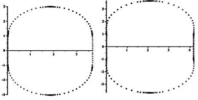
(20) The region of absolute stability (RAS) of the methods (10) and (14) from their respective characteristics equa-tions (19) and (20) are plotted using the maple software in ﬁgures 1 and 2 respectively: Remark: The RAS for

Figure 1: RAS for SDBDF fork= 3 andk= 4

the Second Derivative Backward Diﬀerentiation Formula presented shows that the main methods (10) and (14) are

A-stable for orderp= 4 andp= 5.

4 Implementation Strategy of the

Meth-ods

In what follows, a general procedure for the implemen-tation of the methods using a Boundary Value tech-nique or method in matrix form as in Fatunla [6] is pre-sented. To obtain the approximate solutions for yn+j,

j= 0,1,2,· · ·, N = b−a

h points on the bound of

integra-tion [a, b], with N-vector YN, FN and GN speciﬁed, we

(4)

YN = [yn+1, yn+2, yn+3, ..., yn+N]T

YN−1 = [yn−N+1, yn−N+2, yn−N+3, ..., yn]T

FN = [fn+1, fn+2, fn+3, ..., fn+N]T

GN = [gn+1, gn+2, gn+3, ..., gn+N]T

where yn+j = y(xn +jh), fn+j = f(xn +jh, y(xn +

jh)) and gn+j ≡ df(x,y_dx(x))|yx==xynn++jj. The integration on the entire block shall be written compactly as,

AYN =BYN−1+hCFN +h2DGN (21)

Which forms a non-linear equation because of the implicit nature, hence we employ the Newton-iteration for the evaluation of the approximate solutions. Hence, (21) can be written as,

AYN −BYN−1−hCFN−h2DGN = 0 (22)

Using the Newton’s approach for the implementation of implicit schemes as given in [12], we have that the solu-tions of the block is given as,

Y_N(i+1)=Y_N(i)−J−1 (YN)

AYN−BYN−1−hCFN−h2DGN

(23)

whereJ−1₍_Y

N) the Jacobian matrix is,

J−1₍

YN) =

A−hC∂FN ∂Y −h

2

D∂GN ∂Y

−1

Hence on transformation into matrix form, we have,

AYN =BYN−1+hCFN +h2DGN (24)

such that fork= 2,

A= ⎛ ⎜ ⎜ ⎜ ⎜ ⎜ ⎜ ⎜ ⎝ 64 85 − 86

85 0 · · · 0 0 4

5 −

7

10 0 · · · 0 0 27

85 − 108

85 1 · · · 0 0

0 . .. . .. . .. 0 0

0 0 27₈₅ −108₈₅ 1 0 0 0 0 27₈₅ −108₈₅ 1

⎞ ⎟ ⎟ ⎟ ⎟ ⎟ ⎟ ⎟ ⎠ B= ⎛ ⎜ ⎜ ⎜ ⎜ ⎜ ⎜ ⎜ ⎝

0 0 0 · · · 0 −22₈₅

0 0 0 · · · 0 ₁₀1 0 0 0 · · · 0 ₈₅4

0 0 0 0 0 0

..

. ... ... ... ... ...

0 0 0 0 0 0

⎞ ⎟ ⎟ ⎟ ⎟ ⎟ ⎟ ⎟ ⎠ C= ⎛ ⎜ ⎜ ⎜ ⎜ ⎜ ⎜ ⎜ ⎝

−1 0 −23

85 0 · · · 0

0 −1 2

5 0 · · · 0

0 0 66

85 0 · · · 0

0 0 0 66

85 0 0

0 0 ... 0 . .. 0

0 0 0 0 0 66

85 ⎞ ⎟ ⎟ ⎟ ⎟ ⎟ ⎟ ⎟ ⎠ D= ⎛ ⎜ ⎜ ⎜ ⎜ ⎜ ⎜ ⎜ ⎝

0 0 14₈₅ 0 0 0

0 0 −1₅ 0 0 0

0 0 −18₈₅ 0 0 0

0 0 0 −18₈₅ 0 0

..

. ... ... 0 . .. 0

0 0 0 0 0 −18₈₅

⎞ ⎟ ⎟ ⎟ ⎟ ⎟ ⎟ ⎟ ⎠

and fork= 4, we have,

A= ⎛ ⎜ ⎜ ⎜ ⎜ ⎜ ⎜ ⎜ ⎜ ⎜ ⎝ 891 830 − 3213 1660 549

830 0 · · · 0 0 212

415

229 830 −

916

1245 0 · · · 0 0

−237₈₃₀ 1911₁₆₆₀ 2249₂₄₉₀ 0 · · · 0 0

−₄₁₅64 216₄₁₅ −576₄₁₅ 1 · · · 0 0

0 . .. . .. . .. . .. 0 0

0 0 −64

415 216 415 −

576

415 1 0

0 0 0 −64

415 216 415 − 576 415 1 ⎞ ⎟ ⎟ ⎟ ⎟ ⎟ ⎟ ⎟ ⎟ ⎟ ⎠ B= ⎛ ⎜ ⎜ ⎜ ⎜ ⎜ ⎜ ⎜ ⎜ ⎜ ⎝

0 0 0 0 · · · 0 −333 1660

0 0 0 0 · · · 0 127 2490

0 0 0 0 · · · 0 −187 4980

0 0 0 0 · · · 0 − 9 415

0 0 0 0 · · · 0 0

..

. ... ... ... ... ...

0 0 0 0 · · · 0 0

⎞ ⎟ ⎟ ⎟ ⎟ ⎟ ⎟ ⎟ ⎟ ⎟ ⎠ C= ⎛ ⎜ ⎜ ⎜ ⎜ ⎜ ⎜ ⎜ ⎜ ⎜ ⎝

−1 0 0 ₁₆₆31 0 · · · 0 0 −1 0 −12₈₃ 0 · · · 0 0 0 −1 ₁₆₆51 0 · · · 0 0 0 0 60₈₃ 0 · · · 0

0 0 0 0 60₈₃ 0 0

0 0 0 0 0 . .. 0

0 0 0 0 0 0 60₈₃

⎞ ⎟ ⎟ ⎟ ⎟ ⎟ ⎟ ⎟ ⎟ ⎟ ⎠ D= ⎛ ⎜ ⎜ ⎜ ⎜ ⎜ ⎜ ⎜ ⎜ ⎜ ⎝

0 0 0 −87

830 0 · · · 0

0 0 0 31

415 0 · · · 0

0 0 0 −111

830 0 · · · 0

0 0 0 −72

415 0 · · · 0

0 0 0 0 −72

415 0 0

..

. ... ... ... . .. ...

0 0 0 0 · · · 0 −72

415 ⎞ ⎟ ⎟ ⎟ ⎟ ⎟ ⎟ ⎟ ⎟ ⎟ ⎠

Remark: The boundary value technique with (23) is made possible using the Newton’s iteration features in the maple software.

5 Experimental Problems

In this section we consider some second order non-linear ordinary differential equations of Lane-Emden type (2) which are transformed to system of first order differential equations. The boundary value methods for k = 3 and

k= 4 will be denoted as BVM3 and BVM4 respectively in the presentation of numerical results.

Problem 5.1 White-dwarf Equation: Consider the White dwarf equation,

y′′₊2 xy

′₍_x_{) +}

(5)

introduced in [4] in the study of gravitational potential of the degenerate white-dwarf stars is solved with the BVMs forC= 0.2,0.4,0.6 and 0.8, where atC= 0, (25) becomes the standard Lane-Emden form= 3. (25) can be transformed to the system,

y′₌_z _y_{(0) = 1}

z′₌₋2 xz+

y2−C32

z(0) = 0 (26)

Solving (26) using the BVMs for k = 3 and k = 4 is denoted as BVM3 and BVM4 respectively, the numerical results are compared with the results obtained in [9] and [10] and are presented in Tables 2 and 3, while graphi-cal results is presented forC = 0,0.2,0.4,0.6 and 0.8 in Figure 3 and 4.

Figure 2: Graphical Result for White Dwarf Equation Using BVM3 and BVM4

Table 2: Numerical result for C = 0 using BVM3 for

h= 0.05

x BVM3 BVM4 Hojjati and Parand [9] Horedt [10] 0.5 0.9598393004 0.9598390586 0.959839069883 0.959839 1.0 0.8550578750 0.8550575772 0.855057568546 0.855058 5.0 0.1108196525 0.1108198152 0.110819835160 0.110820 6.0 0.0437378675 0.0437379642 0.043737983910 0.043738

Table 3: Numerical result for C = 0 using BVM3 for

h= 0.01

x BVM3 BVM4 Hojjati and Parand [9] Horedt [10] 0.5 0.9598390702 0.9598390699 0.959839069883 0.959839 1.0 0.8550575691 0.8550575686 0.855057568546 0.855058 5.0 0.1108198348 0.1108198351 0.110819835160 0.110820 6.0 0.0437379836 0.0437379839 0.043737983910 0.043738

Remark: From the Table 2 and 3, it is easily seen that the boundary value methods (BVM3 and BVM4) are comparable to the results obtained in Hojjati and Parand [9] and Horedt [10].

Problem 5.2We also consider the second order diﬀer-ential equation:

y′′₊2 xy

′₍_x_{) + 4}₂_ey₊_ey2

= 0 (27)

Problem (27) has an analytical solution: y(x) =

−2 ln

1 +x2

. To solve (27) numerically, we again recast

it to a system of ﬁrst order ordinary diﬀerential equation of the form,

y′₌_z _y_{(0) = 0}

z′ ₌₋2

xz−4

2ey₊_ey2 z(0) = 0 (28)

The problem is then solved using the derived SDBDF methods by BVM. The Numerical results obtained are presented in Tables 4, 5, 6 and 7 for solution usingh= 0.05 and h = 0.01. Remark: See from Tables 4,

Table 4: Numerical Results for Problem 5.2 for BVM3 usingh= 0.05

x Exact BVM3 Error

0.25 -0.121249243633 -0.121239888642 9.35E-06 0.50 -0.446287102628 -0.446275599224 1.15E-05 0.75 -0.892574205257 -0.892570430056 3.77E-06 1.00 -1.386294361199 -1.386294361120 2.80E-06

x Exact BVM3 Error

0.25 -0.121249243633 -0.121249230231 9.35E-08 0.50 -0.446287102628 -0.446287082373 2.02E-08 0.75 -0.892574205257 -0.892574195535 9.72E-09 1.00 -1.386294361199 -1.386294365367 4.24E-09

x Exact BVM4 Error

0.25 -0.121249243633 -0.121249559058 3.15E-07 0.50 -0.446287102628 -0.446286113311 9.89E-07 0.75 -0.892574205257 -0.892573230121 9.75E-07 1.00 -1.386294361199 -1.386294072225 2.88E-07

5, 6 and 7, that methods of BVM4 performs better than the methods of BVM3, which justiﬁes that the higher the order of convergence of the BVM the higher the accuracy to be expected viz a viz the step length.

Problem 5.3 The ﬁnal example in this paper is also given by:

y′′₊2 xy

′₍_x₎₋₂

2x2+ 3

y= 0 (29)

Equation (29) is of Lane-Emden problem type with an analytical solution given by: y(x) =ex2_{. Equation (29)}

transforms to the system of ﬁrst order ordinary diﬀeren-tial equation given as,

y′₌_z _y_{(0) = 0}

z′₌₋2

xz+ 2

2x2_{+ 3}

y z(0) = 0 (30)

The Tables 8, 9, 10 and 11 shows the numerical results obtained using the BVM3 and BVM4 methods.

(6)

x Exact BVM4 Error

0.25 -0.121249243633 -0.121249243938 3.04E-10 0.50 -0.446287102628 -0.446287102319 3.09E-10 0.75 -0.892574205257 -0.892574204718 5.39E-10 1.00 -1.386294361199 -1.386294361120 3.34E-10

x Exact BVM3 Error

0.25 1.0644944589179 1.0644898251043 4.63E-06 0.50 1.2840254166877 1.2839987348882 2.67E-05 0.75 1.7550546569603 1.7549853685547 6.92E-05 1.00 2.7182818284590 2.7180041217896 2.78E-04

6 Conclusion

We have been able to derive some mixed boundary value methods via the multistep collocation technique. The methods obtained have been represented as a boundary value methods using the representation of block schemes (21). Properties such as order of convergence and re-gion of absolute stability were highlighted using tables and ﬁgures respectively. These BVMs methods were im-plemented on second order nonlinear ordinary diﬀerential equations of Lane-Emden’s Type and their results were found to be sufficiently accurate for various values of step length.

References

[1] Amodio P and Mazzia F., Variable-step boundary value meth-ods based on reverse Adams schemes and their grid distribution, Appl. Numer. Math. 18, 5 - 21, 1995.

[2] Axelsson A. O. H and Verwer J. G., Boundary value techniques for initial value problems in ordinary diﬀerential equations,Math. Comput., 45, 153 - 171, 1985.

[3] Brugnano L. and Trigiante D., Solving Differential Problems by Multitep Initial and Boundary Value Methods, Gordon and Breach Science Publishers, Amsterdam, 1998.

[4] Davis H. T.,Introduction to Nonlinear Differential and Integral Equations, Dover, New York, 1962.

[5] Ehigie J. O., Okunuga S. A. and Sofoluwe A. B., 3-point Block Methods for Direct Integration of Second Order Ordinary Dif-ferential Equations,Advances in Numerical Analysis, Vol. 2011, Article ID 513148, 14 pages, doi:10.1155/2011/513148, 2011.

[6] Fatunla S. O., Parallel methods for Second Order ODEs in Monogragh- Computational Ordinary Differential Equations Ed. By Fatunla S. O., University Press Plc, Ibadan, 87 - 99, 1992.

[7] Hairer E. and Wanner G.,Solving Ordinary Differential Equa-tions II: Stiff and Differential Algebraic Problems, Second Re-vised Edition, Springer Verlag, Germany, 1996.

[8] He J. H., Variational approach to the Lane-Emden equation, Appl. Math. Comput., 143, 539 - 541, 2003.

[9] Hojjati G. and Parand K., An efficient computational algorithm for solving the nonlinear Lane-Emden type equations., Interna-tional Journal of Mathematics and Computer Sciences, 7(4), 182 - 187, 2011.

[10] Horedt G. P.,Polytropes Applications in Astrophysics and Re-lated Fields, Klawer Academic Publishers, Dordrecht, 2004.

[11] Jator S. N. and Sahi R. K., Boundary value technique for initial value problems based on Adams-type second derivative methods, International Journal of Mathematical Education in Science and Education, 1 - 8, iFirst, 2010.

x Exact BVM3 Error

0.25 1.0644944589179 1.0644944535753 5.34E-09 0.50 1.2840254166877 1.2840253903544 2.63E-08 0.75 1.7550546569603 1.7550545627475 9.42E-08 1.00 2.7182818284590 2.7182814883158 3.40E-07

x Exact BVM4 Error

0.25 1.0644944589179 1.0644960766097 1.62E-06 0.50 1.2840254166877 1.2840299847767 4.57E-06 0.75 1.7550546569603 1.7550684409046 1.37E-05 1.00 2.7182818284590 2.7183249275467 4.31E-04

[12] Lambert J. D.,Computational methods in Ordinary Differential Equations, John Wiley and sons, New York, 1973.

[13] Liao S., A new analytic algorithm of Lane-Emden type equations, Appl. Math, Comput., 142, 1- 16, 2003.

[14] Mandelzweig V. B. and Tabakin F., Quasilinearization approach to nonlinear problems in physics with application to nonlinear ODEs,Comput. Phys. Commun., 141, 268 - 281, 2001.

[15] Onumanyi P., Awoyemi D. O, Jator S. N., and Sirisena U. W., New linear mutlistep methods with continuous coefficients for ﬁrst order initial value problems,J. Niger. Math. Soc.13, 3751, 1994.

[16] Okunuga S. A. and Ehigie J. O., A New Derivation of Continu-ous Collocation Multistep methods Using Power Series as Basis Function,Journal of Modern Maths and Statistics, 3, 2, 43 - 50, 2009.

[17] Parand K and Shanini M., Rational Chebyshev Collocation method for solving Nonlinear Ordinary Diﬀerential Equations of Lane-Emden Type, International Journal of Information and Systems Sciences, 6, 1, 72 - 83, 2010.

[18] Parand K., Shahini M. and Dehghan M., Rational Legendre pseu-dospectral approach for solving nonlinear diﬀerential equationds of Lane-Emden type,J. Comput. Phys., 228, 8830 - 8840, 2009.

[19] Ramos J. I., Series approach to the Lane-Emden equation and comparison with the homotopy perturbation method, Chaos. Solit. Fract., 38, 400 - 408, 2008.

[20] Shawagfeh N. T., Nonperturbative approximate solution for Lane-Emden equation,J. Math. Phys., 34, 4364 - 4369, 1993.

[21] Youseﬁ S. A., Legendre wavelets method for solving diﬀerential equations of Lane-Emden type,Appl. Math. Comput., 181, 1417 - 1422, 2006.

x Exact BVM4 Error