Jiri Barnat and Keijo Heljanko (Eds.) 10th International Workshop on
Parallel and Distributed Methods in verifiCation (PDMC 2011) EPTCS 72, 2011, pp. 68–83, doi:10.4204/EPTCS.72.8
c
J. Barnat & P. Bauch & L. Brim & M. ˇCeˇska This work is licensed under the
Creative Commons Attribution License. Jiˇr´ı Barnat
Faculty of Informatics Masaryk University Brno, Czech Republic
Petr Bauch Faculty of Informatics
Masaryk University Brno, Czech Republic
Luboˇs Brim Faculty of Informatics
Masaryk University Brno, Czech Republic
Milan ˇCeˇska Faculty of Informatics
Masaryk University Brno, Czech Republic
Computation of optimal cycle mean in a directed weighted graph has many applications in program analysis, performance verification in particular. In this paper we propose a data-parallel algorithmic solution to the problem and show how the computation of optimal cycle mean can be efficiently accelerated by means of CUDA technology. We show how the problem of computation of optimal cycle mean is decomposed into a sequence of data-parallel graph computation primitives and show how these primitives can be implemented and optimized for CUDA computation. Finally, we report a fivefold experimental speed up on graphs representing models of distributed systems when compared to best sequential algorithms.
1
Introduction
High quality implementation of complex computer systems, e.g. complex embedded systems, is a major challenge today and the computer industry struggles with how to efficiently engineer these systems. Implementations of these systems raise complex parallelism and scheduling issues, which are in practice solved by hand or, at best, by using emerging tools that address only a limited set of applications with favourable properties, such as static nests of loops. One way to tackle this challenge is to use model-driven engineering.
Model-driven engineering is a very active academic domain, driving many studies and prototype tools, and there is an emerging industrial market with an expected growth greater than 10% per year (cf Forrester Consulting). Model-driven performance analysis introduces performance analysis in the early design phases and leading thus to design of more reliable and optimal system.
Inspections of graph cycles is one of the possible means to deal with performance prediction. For example assume that transitions of a system are labelled with resource consumption that the actions these transitions model impose on the system. Then by finding themaximal cycle meanof a graph representing the system it is possible to approximate the worst sustainable load—the amount of resources consumed— under which the system will operate. Unlike using Queueing networks [16] or stochastic Petri nets [20] the computation of optimal cycle mean (OCM) allows to measure the worst expectable performance over infinite runs.
The potential use of the OCM computation for performance analysis should be more apparent with our running example of a client/server distributed application. Provided we are able to create a model of this application with edge-labels representing consumption of CPU resources we intend to compute how many clients will consume how much of the CPU of the server. Analogously, the inspection of properties of critical cycles, and especially the computation of OCM, allows to analyse performance of a large number of systems.
It has been shown that the system to be analysed can be modelled as a Petri net [22], Process graph [19] or e.g. a Data flow graph [15]. When an appropriate modelling formalism for the given real-world system is used, the enumeration of a specific cycle property facilitates performance evalua-tion of asynchronous systems [4], delay intensive and latency-insensitive systems [18]; rate analysis and scheduling of embedded real-time systems [19]; time-separation analysis of concurrent systems [5] and many others. The performance evaluation measures provided by OCM computation include resource consumption (CPU, memory, bandwidth, etc.), worst expectable latency and other measures in specific systems, e.g. cycle period in synchronous systems.
Many different approaches to compute OCM have been taken so far. Dasdan et al. [11] gave a com-prehensive list of algorithms. However, it is imperative that the process of finding the cycles is not overly expensive since many of these applications require the critical cycle to be found repeatedly [10]. To further emphasize the necessity of having efficient algorithmic solution to this problem we present two practical observations. The graphs representing even a small system can be exceedingly large, containing millions of vertices. Moreover, the number of cycles can be exponential with respect to the number of vertices thus making the trivial inspection of all cycles in the graph impractical. Yet the asymptotic com-plexity of even the best sequential algorithms is very high, which renders the applicability of OCM-based performance analysis limited to small systems. We intend to improve the run-time of OCM computa-tion and consequently the applicability of OCM-based performance analysis by employment of SIMD parallelism.
The potential of SIMD parallelism has been recently rediscovered (first efficiently employed in the Connection Machines [13]) with the entry of affordable graphics processing units (GPU) computation. The GPUs possess off-the-shelf data-parallel computation capability, which was soon realized by the academic community and has led to acceleration of various scientific computations. Among these ap-plications of SIMD parallelism were also examples of acceleration of graph algorithms: several can be found in [12], together with thorough experimental evaluation on large sparse graphs.
Since the distributed computation of OCM algorithms has led to rather moderate results [6], we attempt to utilize the massive parallelism of modern GPUs to accelerate the OCM computation. In order to give a lucid description of the procedure we first provide details on what limitations are imposed on the algorithmic solution by the target architecture, i.e. the advantages and shortcomings of modern general purpose GPUs. Subsequently, we choose among the existing algorithms the one most appropriate for data-parallelization through careful inspection of the relative extend of the underlying graph operations. Then we describe the translation of this algorithm and finally conduct an experimental study, comparing our new data-parallel version with the sequential version and also with other sequential algorithms.
2
Preliminaries
Ga Gb
Gc
Gd
(a)G2and its strongly connected components.
Ga Gb
Gc
Gd
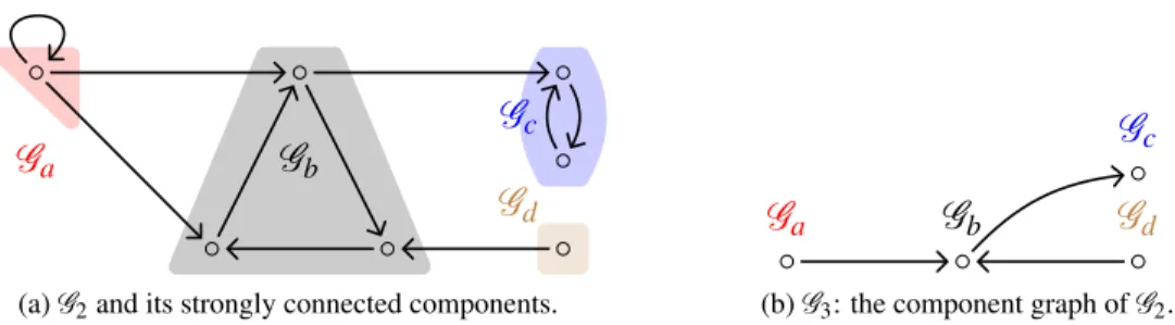
(b)G3: the component graph ofG2. Figure 1: Graph with strongly connected components and the corresponding component graph.
2.1 Related Graph Theory Definitions
Agraphis a tuple G = (V,E), whereV is a set ofverticesandE ⊆V×V. As usual, cardinalities of sets|V|and|E|are denoted withnandm, respectively. ApathinG is a non-empty sequence of edges π=<e1, . . . ,en>such that∀1≤i≤n:ei= (vi−1,vi)∈E. The length of pathπis denoted as|π|and
forπ =<e1, . . . ,en>equals ton. A path for whichv0=vn is called acycle. The set of all cycles of
graphG is denoted withZG.
We say that a graph iscyclicif and only if every edge is part of some cycle. Furthermore, we say that a graph is rooted if there is a root vertexsof the graph such that all the other vertices arereachablefrom it, i.e.∀v∈V there is a path fromstov. Should there be no such a vertex in the graph, weaugmentthe graph be adding a new vertexs∈/V and edges{(s,v)|∀v∈V}.
Let G = (V,E) be a graph. Aweight function is a functionw:E →Rthat assigns a real weight to every edge of G. We speak of weighted graph if G and w are given. Weight function naturally
extends to paths as a sum of the weights of all the edges on the path, i.e. w(π)d f=∑ni=1w(ei), where
π =<e1, . . . ,en>. In the case of augmented graphs we put w(e) =0 for every newly added edge e.
Finally, letπbe a cycle in a graphG weighted with a weight functionw. We definecycle meanof cycle πasµ(π)d f=w|(ππ|). Minimal cycle meanfor a given graphG and weight functionwis then denoted with µ∗(G,w), whereµ∗(G,w) =min{µ(π)|π ∈ZG}. Henceforward, we will safely drop the graph and weight function from the notation of minimal cycle mean and will refer to minimal cycle mean simply as tooptimal cycle meanthat will be denoted byµ∗.
Definition 2.1. OCM problem: For a given graphG and weight function w find the minimal cycle mean.
In order to describe further details of some OCM algorithms we introduce the notion of parametric weight functions and strongly connected components. Given a weight functionwand a real numberΛ,
we defineparametric weight function wΛ d f
=w−Λ. We say thatΛisfeasiblefor a graphG if no cycle in the graph has negative weight with respect towΛ. Directed graphG = (V,E)isstrongly connectedif
∀u,v∈V there is a path fromutov. GraphGs= (Vs,Es)is a maximalstrongly connected componentof G ifVs⊆V,Es⊆Einduced onVs, andVsis a maximal inV such thatGsis strongly connected. Graph Gc= (Vc,Ec)is acomponent graphofG ifVcis the set of all strongly connected components ofG and e= (G1,G2)is inEc⊆Vc×Vcif there is an edge inG between a vertex fromG1and a vertex fromG2. An exemplary illustration of strongly connected components of a graph and its corresponding component graph see Figure 1.
Proposition 2.2. Λis feasible⇔Λ≤µ∗.
2.2 OCM as a Performance Analysis Measure
In order for us to be able to validate the applicability of the OCM computation as a performance analysis measure we have extended the DIVINE model checking tool with the possibility of OCM computation. Originally, the explicit state space, parallel model checker DIVINE has in its core an algorithm for com-putation of accepting cycle. Preserving most of the code, especially the part generating the transition system, we only needed to perform a few changes in the modelling language and to replace accepting cycle detection algorithms with OCM algorithms.
DVE, the modelling language of DIVINE, allows specification of communicatingprocessesin a very intuitive fashion. From the general point of view the processes consist ofstatesand we usetransitions to move from one state to another. The communication is achieved bysynchronizationof two transitions from different processes: we require these two transition to be executed concurrently in the resulting transition system. To allow performance evaluation we have added specification of cost and time to every transition. The cost can represent consumption of some resource of computation (CPU utilization, memory requirements, etc.) and the addition of time allows to compute the more general optimal cycle ratio [19].
The primary motivation behind the extension of DIVINE was performance analysis of an online PDF editor that was, in the time of writing, being developed by the Normex company. The OCM-based analysis was used with the intention to measure the worst expectable utilization of the CPU server. For the analysis to be as precise as possible we have devised several scenarios of the behaviour of the clients and constructed the model as a synchronous composition of these scenarios. Specifics of the scenarios were determined based on results of a case study among users of a similar editor and on preliminary beta testing. The concrete findings of our analysis will be detailed in Section 4.
2.3 CUDA Computation
The Compute Unified Device Architectures (CUDA) [9], developed by NVIDIA, is a parallel program-ming model and a software environment providing general purpose programprogram-ming on Graphics Processing Units. At the hardware level, GPU device is a collection of multiprocessors each consisting of eight scalar processor cores, instruction unit, on-chip shared memory, and texture and constant memory caches. Ev-ery core has a large set of local 32-bit registers but no or a vEv-ery small cache (L1 cache has configurable size of 16-48KB). The multiprocessors follow the SIMD architecture, i.e. they concurrently execute the same program instruction on different data. Communication among multiprocessors is realized through the shared device memory that is accessible for every processor core.
On the software side, the CUDA programming model extends the standard C/C++ programming language with a set of parallel programming supporting primitives. A CUDA program consists of ahost code running on the CPU and adevicecode running on the GPU. The device code is structured into the so calledkernels. A kernel executes the same scalar sequential program in manyindependent data-parallel threads.
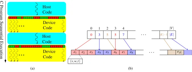
Each multiprocessor has several fine-grain hardware thread contexts, and at any given moment, a group of threads called awarpexecutes their instructions on the multiprocessors in a lock-step manner. When several warps are scheduled on multiprocessors, memory latencies and pipeline stalls are hidden primarily by switching to another warp. Overall the combination of out-of-order CPU and data-parallel processing GPU allows for heterogeneous computation as illustrated in Figure 2a, where sequential host code and parallel device code are executed in turns.
Device Code Host Code
Device Code Host Code
C Program Sequential Execution
(a)
0 1 2 3 4 |V|
. . .
0 3 5 5 7 |E|−1 |E|
e1 e2 e3 e4 e5 e6 e7 e8
. . .
e|E|(v,w,t)
(b)
Figure 2: a) Sequential heterogeneous computation work-flow with CUDA. b) Adjacency list represen-tation: a graphG= (V,E)is stored as two arrays:Aiof size|V|+1 andAt of size|E|.
have to allow independent thread-local data processing so that the CUDA hardware can fully utilize its massive parallelism. And second, they have to be small so that the high latency device-memory access and limited device-memory bandwidth are not large performance bottlenecks (also the regularity of structures in the memory is of great importance). In our case, it is the representation of graphG to be encoded appropriately in the first place. Note that uncompressed matrix or dynamically linked adjacency lists violate these requirements and as such they are inappropriate for CUDA computation.
An efficient CUDA-aware computation of a graph algorithm requires the graph to be represented in a compact, preferably vector-like, fashion. We encode the graph as an adjacency list that is represented as two one-dimensional arraysAtandAi, similarly as in [12]. The arrayAt keeps target vertices of all the
edges of the graph. The target vertices stored in the array are ordered according to the source vertices of the corresponding edges. The secondAi array then keeps an index to the first array for every vertex in
the graph. Every index points to the position of the first edge (represented as a target vertex) emanating from the corresponding vertex. See Figure 2b. If other data associated to a vertex are needed by a CUDA kernel algorithm, then they are organized in vectors as well.
Most of known OCM algorithms require to access predecessors of a given vertex in order to perform a kind of backward reachability. Storing backward edges together with their forward versions causes additional nontrivial memory requirements, which might be a problem as the size of CUDA memory is limited. We have shown how to carry out the backward reachability using only forward edges with minor time overhead [2]. However, OCM algorithms often require the reachability procedure to perform only on a given subgraph of the whole graph (such that it contains a single outgoing edge for every vertex). Unfortunately, augmenting the original procedure proposed in [2] in order to follow the selected edges only resulted in considerable slow down in computation. For that reason we were forced to explicitly store both forward and backward edges of the graph.
Algorithm 1:Scanning Method of SPF Algorithms
Input: Afoundvertexu
1 foreache= (u,v)∈E do 2 ifπ(u) +w(e)<π(v)then
3 π(v),p(v),S(v)←π(u) +w(e),u,found
4 S(u)←scanned
2.4 OCM Algorithms
Through the course of study of optimal properties of graph cycles a plethora of algorithms emerged. These algorithms, while not sharing similar concepts, can be divided into several groups according to what graph property they use to find critical cycles. Since our goal in this section is to choose one of the algorithms which would be most suitable for data-parallel implementation we will describe all three categories of OCM algorithms and consider their aptness for our purpose.
There are various limitations imposed on the potential algorithms should they be even considered for SIMD acceleration. First of all, most of the data structures used should be to a very large extend in form of vectors: stacks, queues or heaps are not possible to be effectively data-parallelized. Then the kernels should prevalently address the whole set of vertices (or edges): limiting the computation to a insufficiently small subset would prevent utilization of the computational power. Yet the vector-wide operations are rather costly even on many-core architectures and the complexity of algorithms is practically measurable in their number. Finally, there is also a non-negligible overhead of kernel calls and thus even a very fast kernel should not be run excessively.
A strong relation can be observed between the OCM and theShortest Path Feasibility(SPF) prob-lems [10]. This relation should be much more apparent once we formulate the OCM problem as a linear programming problem: µ∗is the optimal solution of
maxrsubject to
d(v)≤d((u) + (w((u,v))−r) ∀e= (u,v)∈E,
(1)
wheredstands fordistance, i.e. minimal-cost path from the source node tov. According to the previous formulation, we can equivalently search for the maximal parameterr such thatG withwr contains no negative cycle. Following Proposition 2.2 suchris exactly the optimal cycle mean. As a result, existence of an efficient implementation of the SPF algorithm enables an efficient solution to the OCM problem. Furthermore, any future improvements to the SPF procedure automatically translates to improvements in this OCM problem solution.
All SPF algorithms have a common basic step: the scanning method [8]. This method assumes we maintain for every vertex uits potential π(u), parent p(u), and a label S(u)∈ {unreached,found,
scanned}. Initially, only the root vertex is labelledfound, all other vertices areunreached, and potential of all vertices is set to zero. A singlefoundvertex is then repeatedly scanned using Algorithm 1.
The scanning method repeats until there are nofoundvertices or until the algorithm finishesn passes. Recall thatn=|V|. Passes of an SPF algorithm are defined inductively:
0-th pass is the initialization,
If allnpasses are performed, the graph inevitably contains a negative cycle.
2.4.1 Cycle-Based
The arguably most straightforward application of shortest path feasibility solution to the OCM problem is thecycle-based approach. The idea is to maintain an upper boundΛof the minimal cycle mean, i.e.
Λ≥µ∗, and a cycleCsuch thatΛ=µ(C). IfΛ>µ∗then new better upper boundΛ′of minimal mean cycle can be detected with the SPF algorithm provided that it uses parametric weight functionwΛ. The
newly computed upper boundΛ′is used in another iteration of the algorithm asΛ. The whole procedure
repeats until no improvement of upper bound can be found, which indicates thatΛ=µ∗.
A classical implementation of the cycle-based approach is the Howard’s algorithm [14], which further improves the approach by altering the SPF procedure. At the end of each pass it checks the parent graph, induced by edges(p(v),v), for cycles. Existence of a cycle allows to restateΛto a value that sets to zero the weight of the most negative cycle. Should there be no negative cycle the improved SPF algorithm either terminates, if all reduced weights are non-negative, or it continues with the next pass.
The cycle-based approach seems to be fairly compatible with the SIMD computation. Namely, the SPF subroutine is a vector-wide propagation of values, the minimal cycle location on the parent graph is also feasible to parallelize, and most importantly sequential experiments suggest that the algorithm typically performs only very few passes of the underlying SPF subroutine.
2.4.2 Binary Search
Thebinary searchapproach is slightly more involved. It maintains both upper and lower boundΛ1≤ µ∗ ≤Λ2 together with a cycleC such that µ(C) =Λ2. The SPF subroutine is repeatedly called with
parametric weight functionwΛ, whereΛ, as the name suggests, is set to Λ1+2Λ2. In case a negative cycle
ζ is found, we set C andΛ2 toζ andµ(ζ), respectively. Since we did not useΛ2 as a parameter we cannot be certain of the value of the optimal cycle mean in either of SPF answers, and thus if no negative cycle is found we setΛ1toΛ. The termination criterion for binary search approach isΛ2−Λ1<ε. Ifε is chosen sufficiently small,Cwill be the critical cycle.
The well-known implementation of binary search is due to Lawler [17], who also proved the run-time of his algorithm to be inO(nmlg(W/ε)), whereW is the maximal edge weight. Structurally, there is no apparent reason why the Lawler’s algorithm should be inappropriate for data-parallelization, yet the fact that the SPF subroutine requires up tonpasses (and given the idea of binary search it often is necessary to carry out allnpasses) renders this particular approach unusable. This hypothesis was experimentally confirmed once we have implemented the Lawler’s algorithms and executed preliminary tests.
2.4.3 Tree-Based
While the previous two approaches used full SPF, the tree-based approach uses the shortest path fea-sibility subroutine only partially. Here only the lower bound Λ is maintained, initially small enough
to guarantee that all edges have positive weight underwΛ. Λis progressively increased throughout the
algorithm in correctly chosen increments, until a cycleζ is found such thatwΛ(ζ) =0. Apart fromΛ
we also maintain the shortest path treeT, with respect to the currentwΛ. As we are working with the
augmented graph we may initiateTto consist of the edges fromsto every other vertex.
end we assign to every vertexuathreshold, the smallestλ that would forceuto change parent. Finding the smallest among all thresholds is facilitated by a priority queue.
Again this approach is unsuitable for SIMD acceleration for several reasons. The usage of priority queues (either heaps or Fibonacci heaps) is particularly problematic and would most likely be imple-mented as a simple vector, with the minimum operation as parallel reduction. Also the span of operation updating the shortest path tree is in many cases relatively small and would not fully utilize the number of GPU cores. Much larger problem was found during experiments with sequential version demonstrating that there are simply too many iteration of the algorithm that must be carried out one after another.
2.5 Howard’s Algorithm
Since it is the Howard’s algorithm that appears to be the one most suitable for parallelization, we will now provide its detailed description. First, we should stress that the algorithm works on strongly connected graphs only. There exist two approaches how to overcome this restriction. First, we can decompose the given graph to its strongly connected components and then process the graph one component at a time. In the sequential case we can use the Tarjan’s algorithm [23] based on the depth-first traversal procedure which outputs the list of all strongly connected component inO(n+m)time. Hence there is asymptotically no difference in complexity of the algorithm, although practically the difference can be quite substantial. The second approach suggests to modify the underlying graph by adding a Hamiltonian cycleζH =<(v0,v1), . . .(vn−1,v0)>to the graph. With this modification the graph becomes strongly connected and provided that weights of newly added edges are sufficiently large, the optimal cycle mean of the graph remains unchanged.
As stated in the description of the cycle-based approach, the Howard’s algorithm (see Algorithm 2, adopted from [6]) extends the shortest path feasibility algorithm. Indeed the main cycle on lines 7–27 up to line 14 is in fact a scanning step of the SPF algorithm. Altough the output of the cycle on lines 9–13 is not yet the shortest path tree, since we are approaching the optimal cycle mean from top and hence there are cycles in our shortest path graph. To remain consistent with the established notation we will call the graph induced on edges(v,π(v))thepolicy graph.
Apart from the successor in the policy graphπ(v)that must exist since we are working with strongly-connected graphs only, we also store two valuesval0(v)andval1(v)with every vertex. In these two values we keep information about the current and the following parametric length for a given vertex. In every iteration of the out-most cycle we check whether there was a change in the policy graph, and if not we interrupt the main cycle and returnλ as the optimal cycle mean. Eachλ that is used as a parameter for the feasibility computation, is actually the mean weight of a specific cycle in both the original and the policy graph. Hence, after every iteration of the SPF algorithm part we inspect the policy graph, locate all cycles inside it and choose the one with minimal mean weight (line 16). Upon finding the minimal cycle (or after choosing one of the minimal cycles), we modify the policy graph in such a way that every vertex has a path to the minimal cycle (line 18).
Algorithm 2:Howard’s Algorithm
Input : A directed, strongly-connected graphG = (V,E,w),w:E→Q Output:λ∈Q:λ=µ∗(G)
1 foreachv∈V do 2 val0(v)←0
3 π(v)←nil
4 improved←true
5 i←0 6 λ ←0
7 whileimproveddo
8 improved←false
9 foreachv∈V do
10 val((i+1) mod 2)(v)←minu∈Succ(v){val(i mod 2)(u) +w(v,u)−λ}
11 ifπ(v) =nil∨(val(i mod 2)(π(v)) +w(v,π(v))−λ >val((i+1) mod 2)(v))then
12 π(v)←u|val(i mod 2)(u) +w(v,u)−λ =val((i+1) mod 2)(v)
13 improved←true
14 i←i+1
15 ifimprovedthen
16 c←MinMeanWeightCycle(Gπ) // Gπ.|E|=|V|,∀v∈V :deg(v) =1
17 λ←µG(c)
18 break all other cycles thancinGπ so that all vertices have path toc 19 s←MinVertex(c)
20 val(i mod 2)(s)←0
21 q.push(s)
22 while¬q.empty()do 23 v←q.pop()
24 foreachu∈Pred(v)do 25 ifu6=s∧π(u) =vthen
26 val(i mod 2)(u)←val(i mod 2)(v) +w(u,v)−λ
27 q.push(u)
28 returnλ
one to connect also the remaining vertices to the minimal cycle.
Subsequently, we choose one vertex (line 19) on the minimal cycle and set its val to zero. It is necessary that we always select the same vertex, assuming the same cycle is found minimal. After the modification of the policy graph and selecting newλ, it is also necessary to modify theval values for other vertices accordingly. This process is started by setting thevalofsto zero on line 20 and carried out by the cycle on lines 22–27, performing backward reachability fromsalong the edges of the policy graph. In the next iteration of the out-most cycle we again find the policy graph (using the updatedval
Algorithm 3:Howard’s Algorithm – GPU (host code)
Input : A directed, strongly-connected graphG = (V,E,w),w:E→Q Output:λ∈Q:λ=µ∗(G)
1 whiletruedo
2 ifgTerminate←SPFPassIter(G,val,λ,Gπ,it)then break
3 it+ +
4 GpiPreprocess(Gπ,gPredInfo) 5 elimination∗(Gπ,gPredInfo) 6 cycleIdentification(Gπ,gCycles) 7 reducemin(gCycles,minCycle)
8 λ ←minCycle.mean
9 setMinCycle(Gπ,gCycles,minCycle) 10 markMinComponent∗(Gπ,gPredInfo) 11 connectGpi∗(G,Gπ)
12 val[it&1][minCycle.minIndex]←0 13 GpiPreprocess(Gπ,gPredInfo)
14 valuePropagate∗(G−1,Gπ,val[it&1],λ,minCycle.minIndex,gPredInfo)
15 return
3
Data-Parallel Version of Howard’s Algorithm
The actual description of our data-parallel implementation of Howard’s algorithm will be conducted in several steps. We start by proposing a high-level work flow, where we attempt to preserve the provably correct layout. Concurrently proposing graph primitive operations that would perform actions function-ally equivalent to those of the original algorithm, but, wherever possible, addressing the whole vector of values at a time. CUDA-specific implementation of these graph primitives will be detailed extensively in the following section. Finally, we propose an extension to Howard’s algorithm which prepends a parallel decomposition to strongly connected components to the algorithm. Then we let the algorithm perform the OCM computation on all components concurrently.
3.1 High-Level Description
The proposed host code of our implementation is listed as Algorithm 3. It is apparent that lines 16 and 18 of Algorithm 2 that rebuild the policy graph, require much more attention in the SIMD environment as it is the place most susceptible to inefficient processing. These two lines of CPU pseudo-code span from line 4 to line 11 in our GPU implementation. We first describe this part of the algorithm postponing the SPF subroutine for later discussion.
required because of the eliminationandmarkMinComponent kernel, the second call is because of
valuePropagatekernel.
From the description of sequential Howard’s algorithm we know that the policy graph consists of weakly connected components, each containing a cycle and several paths leading to this cycle. In or-der to be able to find all cycles in the policy graph in as few parallel steps as possible, we first apply
eliminationto remove all vertices that do not lie on any cycle, i.e. those that are on the paths leading to a cycle (path vertices). This kernel is called iteratively (every call removes the vertices with no prede-cessors) until a fixpoint is found; in other words until there are no such vertices. There are more fixpoint kernels in Algorithm 3 all marked with an asterisk. The elimination allows localization of cycles and computation of their means in a straightforward manner (line 6): we simply follow the propagation of edges starting from any not eliminated vertex. The minimal among them can subsequently be found by employing parallel reduction [7] withminoperation.
Upon finding the cycle with minimal mean (which for technical reasons has to be agreed on by all vertices: line 9) we can actually start rebuilding the graph. With the first backward reachability (line 10) we undo the elimination of the path vertices within the component of the minimal cycle, hence the second backward reachability (line 11) is started from this component and is iteratively applied until all vertices are connected, one breadth-first search layer at a time.
Finally, the SPF subprocedure is easy to parallelize. Using twovalvectors, alternating the two in odd and even iterations, allows us to perform all updates of values in a single parallel step (as there is no danger of race between threads, see lines 2, 3 and 14). Also realization of the kernelvaluePropagateon line 14 that propagates the change ofvalfrom the vertex on minimal cycle with smallest index (source), was only a minor modification of backward reachability procedure.
3.2 Graph Primitives and Data Structures
We first focus on the data structures that are used during the computation. The graph representation itself has been described in Section 2.3. In order to keep low space profile, we store the policy graphGπ in a vector ofnelements containing indices of theMcarray that uniquely specifies what edge leads to the
successor of a given vertex. Also the first few bits of every element are reserved to flags. For example there is a flag marking what vertices have been removed during elimination. Cycles are stored ingCycles using two 32-bit values, one for the index of its source vertex and second for the mean weight. Finally, the vectorgPredInfois used to store a partial information about the predecessors within one 32-bit value. The first 16-bits are for the number of predecessors and the last 16-bits for thelocalindex of the first predecessor.
While most of our kernels are only minor modifications of previously published data-parallel graph primitives (see e.g. [2]), they are crucial for the overall efficiency of our data-parallel implementation, and therefore, we describe some of those modifications in detail. TheGpiPreprocessprimitive was devised for a simple reason: there is no efficient way to propagate along backward edges in the policy graph. Using forward edges would require deployment of as many threads as there are unseen vertices. Searching among backward edges those in the policy graph, on the other hand, suffers from the fact that there are often as many edges that do not belong to the policy graph. Hence both these approaches are approximately equally inefficient. The improvement we have proposed first passes the whole graph G storing correctly the information about predecessors within the policy graph intogPredInfo. This preprocessing allows to virtually skip inspection of vertices with no predecessors in the policy graph and also to jump at the first edge that belongs to the policy graph as can be observed from the pseudo-code of
Algorithm 4:valuePropagate(G = (Mn,Mc),Gπ=Mπ,val,λ,source,gPredInfo)
1 index←threadId
2 prop←false
3 counter←gPredInfo[index].getNum()
4 pred←Mn[index+gPredInfo[index].getFirst()]
5 whilecounter>0do 6 edge←Mc[pred]
7 ifindex=Mc[Mπ[edge.to]]then
8 counter− −
9 ifedge.to6=sourcethen
10 val[edge.to]←val[index] +edge.weight−λ
11 prop←true
12 pred+ +
13 ifpropthen
14 fixPoint←false
of the vertex assigned to this thread (line 3) and can skip the cycle ifcounteris zero. Together with the jump to the first actual predecessor (see line 4) this improvement alone has led to fivefold speedup of
valuePropagateincluding the cost of preprocessing.
Details on remaining kernels are as follows. eliminationkernel is actually thetrimmingprimitive (see [2]) augmented similarly as the valuePropagate with the information about predecessors. A simple while loop (it is executed only on vertices on some cycle) for identification of cycle source and its mean is implemented in thecycleIdentificationkernel. And finally theconnectGpiperforms backward reachability from the component of the minimal cycle, and it utilizes a flagpropagatewhich marks the currently active breath-first layer. Only the threads that have a vertex with thepropagateflag do propagate and so less threads needs to be dispatched.
3.3 SCC Decomposition Extension
Algorithm 5:Region-specific minimum voting
1 myCycle←(source,mean= (weight/length))
2 whiletruedo
3 comCycle←cycles[myRegion]
4 ifcomCycle.mean≤myCycle.meanthen break
5 atomicCAS(&(cycles[myRegion]),comCycle,myCycle)
component-specificλ values during the computation (which also has to be agreed on).
Selecting the minimal cycle mean during the computation on multiple regions is particularly prob-lematic as the vertices of one component are not clustered together. It would actually require first to split [21] the vector according to the region identification and then perform segmented reduction [7], both complicated and expensive operations. Fortunately, we have observed that often very few cycles are found and consequently only a few values are candidates for the minimum. Thus we were able to use the
atomicCASoperation as shown in Algorithm 5 without any significant time expense.
Also the termination needs to be modified to work on two levels. The global termination occurs when computation is finished on all strongly connected components. But it is also important to prevent execution of kernels on components where we have already found the OCM. Since then less threads needs to be deployed and less candidates compete in the minimum voting. For that purpose we have inserted a kernel that unsets the flagworkfor all vertices in inactive components between lines 2 and 3 of Algorithm 3. Finally, we have optimized the overall amount of work by unsetting theworkflag of all single vertex components prior to the actual OCM computation.
4
Experimental Evaluation
Since the prime objective of our research was to accelerate performance analysis based on computation of optimal cycle mean, we have compared sequential and data-parallel algorithms mainly on models of communicating distributed systems. The state space of all possible configurations of a given system forms a graph with cost function (representing for example resource consumption) labelling edges of that graph. Both modelling of the system and generation of its state space was facilitated by the enumerative model checker DiVinE [3], extended with the capability to analyse performance of input models.
The sequential OCM algorithms Howard’s and YTO were also implemented within DiVinE. Thus the evaluation of our GPU Howard’s algorithm is conducted by comparing its running time against these two sequential algorithms (which are often considered to be the fastest [10]). The graph representation, while primarily targeting the vector processing architecture of GPU, is also particularly suitable for CPU due to its cache-efficient characteristics.
All experiments were executed on a CUDA-equipped Linux workstation with an AMD Phenom II X4 940 Processor @ 3GHz, 8 GB DDR2 @ 1066MHz RAM and NVIDIA GeForce GTX 480 GPU with 1.5 GB of GDDR5 memory. All codes were compiled with-O3optimization using gcc version 4.3.2 and nvcc version 3.1 for CPU and GPU code, respectively.
0 2000 4000 6000 8000 10000 12000
1e+10 1e+11 1e+12 1e+13 1e+14
Time (msec.)
Graph size: n*m YTO
Seq. Howard GPU Howard
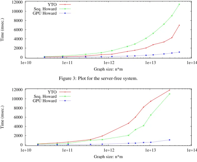
Figure 3: Plot for the server-free system.
0 2000 4000 6000 8000 10000 12000
1e+10 1e+11 1e+12 1e+13 1e+14
Time (msec.)
Graph size: n*m YTO
Seq. Howard GPU Howard
Figure 4: Plot for the system with a server.
information of how many clients of what scenario there are. As stated in Section 2.2 we have used a similar approach in our running example for analysis of CPU utilization in an online PDF editor (as we could for any distributed client/server application in general). After modelling the system using the client scenarios we have computed the maximal cycle mean in the transition system generated from the synchronous composition of those clients. This value was equal to the worst sustainable CPU utilization during any infinite run of the modelled system. Thus we were able to estimate the number of clients that would be able to fully utilize the server.
In order to measure scalability of the GPU algorithm we have constructed two distributed client/server systemtemplatesfrom which a user can generate system models by deciding on the number of client for each scenario. In the first system, there is no server present and the actions of clients are left to be inter-leaved nondeterministically. The second systems contain a server and the clients have to communicate with the server (and only one client can access the server at a time). The OCM of such systems then represents the average system load inflicted on the environment.
size of the graph inn∗mas all the sequential OCM algorithms are asymptotically inO(nm) or worse. Actual sizes of the analysed graphs range from 50 thousand vertices and 400 thousand edges to approxi-mately 2 million vertices and 25 million edges. The plots show very clearly that while both YTO and the sequential Howard’s algorithm struggle with preserving their running times as the graphs grow bigger, our GPU implementation is capable of performing the OCM computation in reasonably small time. On larger instances the GPU rarely fails to provide a fivefold speed up compared to the better of the two se-quential algorithms. It is worth noting that while the CPU algorithms were deterministic and in different runs exhibited indistinguishable behaviour, the GPU implementation behaves nondeterministically due to the nature of the massive parallelism. For that reason we executed every test ten times and the result displayed in the plots is the median of all trials.
Although primarily targeting acceleration of OCM computation for performance analysis we feel obliged to admit that on graphs from other applications was our data-parallel implementation much less successful. We have conducted several experiments with US traffic network graphs, random graphs and various graphs from the DIMACS challenge and were never able to outperform the YTO algorithm. On these graphs the YTO performed only a very few iterations which we attach to the fact that the OCM of these algorithms was often very close to the minimal edge weight.
5
Conclusion
We have proposed data-parallel acceleration of an OCM algorithm within several consecutive steps. First we have evaluated all existing classes of OCM algorithms with respect to their predisposition for vec-tor processing. Subsequently, we have described thoroughly the Howard’s algorithm which was found most appropriate for GPU acceleration and devised its data-parallel version. Specifics of the implemen-tation together with selected data-parallel graph primitives were then detailed, e.g. the incorporation of SCC decomposition and the concurrent execution of the OCM algorithm on all strongly connected components.
The primary motivation behind GPU implementation of OCM algorithms was the acceleration of performance analysis of distributed communication systems. That we have evaluated experimentally by constructing two scalable client/server systems based on distinct scenarios of the clients finding our data-parallel algorithm capable of providing performance analysis in negligible time. Although com-petitiveness of the GPU algorithm on other types of graphs is questionable, we have reported a steady fivefold speed up on performance analysis graph against all other algorithms.
References
[1] J. Barnat, P. Bauch, L. Brim & M. ˇCeˇska (2010): Employing Multiple CUDA Devices to Accelerate LTL Model Checking. In: Proceedings of the 16th International Conference on Parallel and Distributed Systems, IEEE Computer Society, Los Alamitos, CA, USA, pp. 259–266, doi:10.1109/ICPADS.2010.82.
[2] J. Barnat, P. Bauch, L. Brim & M. ˇCeˇska (2011): Computing Strongly Connected Components in Parallel on CUDA. In: Proceedings of the 25th IEEE International Parallel & Distributed Processing Symposium (IPDPS’11), IEEE Computer Society, pp. 541–552.
[3] J. Barnat, L. Brim, M. ˇCeˇska & P. Roˇckai (2010):DiVinE: Parallel Distributed Model Checker (Tool paper). In:Proceedings of joint HiBi/PDMC workshop, HiBi/PDMC 2010, IEEE, pp. 4–7.
[5] S. M. Burns, H. Hulgaard, T. Amon & G. Borriello (1995): An Algorithm for Exact Bounds on the Time Separation of Events in Concurrent Systems. IEEE Transaction on Computers 44(11), pp. 1306–1317, doi:10.1109/12.475126.
[6] J. Chaloupka (2006):Distributed Algorithms for the Minimum Mean Weight Cycle Problem. Master’s thesis, Masaryk University, Faculty of Informatics, Brno.
[7] S. Chatterjee, G. E. Blelloch & M. Zagha (1990):Scan Primitives for Vector Computers. In:Proceedings of the 2nd International Conference for High Performance Computing, Networking, Storage and Analysis (SC ’90), IEEE Computer Society, Los Alamitos, CA, USA, pp. 666–675.
[8] B. V. Cherkassky, L. Georgiadis, A. V. Goldberg, R. E. Tarjan & R. F. Werneck (2010): Shortest Path Feasibility Algorithms: An Experimental Evaluation. Journal of Experimental Algorithmics14, pp. 118– 132.
[9] (April 2011):NVIDIA CUDA Compute Unified Device Architecture - Programming Guide Version 4.0. [10] A. Dasdan & R. K. Gupta (1997): Faster Maximum and Minimum Mean Cycle Algorithms for System
Per-formance Analysis. IEEE Transactions on Computer-Aided Design of Integrated Circuits and Systems17, pp. 889–899, doi:10.1109/43.728912.
[11] A. Dasdan, S. S. Irani & R. K. Gupta (1999):Efficient algorithms for optimum cycle mean and optimum cost to time ratio problems. In:Proceedings of the 36th annual ACM/IEEE Design Automation Conference, DAC ’99, ACM, pp. 37–42, doi:10.1145/309847.309862.
[12] P. Harish & P. Narayanan (2007):Accelerating Large Graph Algorithms on the GPU Using CUDA. In:High Performance Computing (HiPC’07),Lecture Notes in Computer Science4873, Springer Berlin / Heidelberg, pp. 197–208, doi:10.1007/978-3-540-77220-0 21.
[13] W. D. Hillis (1987): The Connection Machine. Scientific American 256(6), pp. 108–115, doi:10.1038/scientificamerican0687-108.
[14] R. A. Howard (1960):Dynamic Programming and Markov Processes. MIT Press, Cambridge, MA.
[15] K. Ito & K. K. Parhi (1995): Determining the Minimum Iteration Period of an Algorithm. The Journal of VLSI Signal Processing11(3), pp. 229–244, doi:10.1007/BF02107055.
[16] L. Kleinrock (1975):Queueing Systems, Volume 1: Theory. Wiley-Interscience, New York.
[17] E. L. Lawler (1976): Combinatorial Optimization: Networks and Matroids. Holt, Reinhart, and Winston, New York, NY.
[18] R. Lu & C. Koh (2006): Performance Analysis of Latency-Insensitive Systems. IEEE Trans-actions on Computer-Aided Design of Integrated Circuits and Systems 25(3), pp. 469–483, doi:10.1109/TCAD.2005.854636.
[19] A. Mathur, A. Dasdan & R. K. Gupta (1998): Rate Analysis for Embedded Systems. ACM Transaction on Design Automation of Electronic Systems3(3), pp. 408–436, doi:10.1145/293625.293631.
[20] M. K. Molloy (1982):Performance Analysis Using Stochastic Petri Nets. IEEE Transactions on Computers
31(9), pp. 913–917, doi:10.1109/TC.1982.1676110.
[21] S. Patidar & P. J. Narayanan (2009): Scalable Split and Gather Primitives for the GPU. Technical Report IIT/TR/2009/99, Centre for Visual Information Technology, Hyderabad, INDIA.
[22] C. V. Ramamoorthy & G. S. Ho (1980):Performance Evaluation of Asynchronous Concurrent Systems Using Petri Nets.IEEE Transaction of Software Engineering6(5), pp. 440–449, doi:10.1109/TSE.1980.230492.