Convergence Analysis of Some New
Preconditioned AOR Iterative Methods for
L
-matrices
Zhengge Huang
∗, Ligong Wang, Zhong Xu and Jingjing Cui
Abstract—In this paper, we present a new preconditioner which generalizes two known preconditioners proposed by Wang et al. (2009) and A. J. Li (2011), and prove that the convergence rate of the AOR method with the new precondi-tioner is faster than the precondiprecondi-tioners introduced by Wang et al. Moreover, we propose other two new preconditioners and study the convergence rates of the new preconditioned AOR methods for solving linear systems. Comparison results show that the new preconditioned AOR methods are better than those of the preconditioned AOR methods presented by J. H. Yun (2011) and A. J. Li (2012). Finally, numerical experiments are provided to confirm the theoretical results studied in this paper.
Index Terms—preconditioner, preconditioned AOR method, Linear system, AOR method,L-matrices.
I. INTRODUCTION
S
OLUTIONS of linear systems arise from the scientific computing and engineering technique, such as solv-ing the steady incompressible Navier-Stokes problem [1], preconditioning techniques for large sparse systems arising in finite element limit analysis [2], multigrid method for linear complementarity problem and its implementation on GPU [3], fourth-order singly diagonally implicit Runge-Kutta method for solving one-dimensional Burgers’ Equation [4] and so forth. So, research of methods for solving linear systems has important theoretic significance and practical applications. In this paper, by constructing three new pre-conditioners and combining with the theories of nonnegative matrices, we will conduct further research in preconditioned AOR iterative methods for solving linear systems. In theory, we prove that the convergence rates of the AOR method with the new preconditioners are faster than the existing ones. To illustrate our results, some numerical experiments are given.Consider the following linear system
Ax=b, (1)
whereA∈Rn×n,b∈Rnare given andx∈Rnis unknown. For simplicity, we let A = I−L−U, where I is the identity matrix,LandU are strictly lower and strictly upper triangular matrices, respectively. Then the iteration matrix of
Manuscript received November 03, 2015; revised January 04, 2016. This work was supported by the National Natural Science Foundations of China (No.11171273).
*Zhengge Huang, Corresponding Author, is with the Department of Ap-plied Mathematics, Northwestern Polytechnical University, Xi’an, Shaanxi, 710072, PR China. e-mail: [email protected].
Ligong Wang (e-mail: [email protected]),Zhong Xu (e-mail: [email protected]) and Jingjing Cui (e-mail: [email protected]) are with the Department of Applied Mathematics, Northwestern Polytech-nical University, Xi’an, Shaanxi, 710072, PR China.
the AOR iterative method [5] for solving the linear system (1) is
Lr,w= (I−rL)−1[(1−w)I+ (w−r)L+wU], (2)
wherew andrare real parameters with w6= 0.
In order to accelerate the convergence of iterative method for solving the linear system (1), the original linear system (1) is transformed into the following preconditioned linear system
P Ax=P b, (3)
whereP is called a preconditioner, is a nonsingular matrix. The preconditioned system (3) with the different precondi-tionersP have been proposed by many authors [6], [7], [8], [9], [10], [11], [12], [13], [14], [15], [16], [17], [18], [19], [20], [21].
In 2009, Wang and Li [6] and in 2011, A. J. Li [7] presented preconditionersP˜ =I+ ˜Sα,β andPˆ=I+ ˆSα,β forL-matrices, respectively, where
˜
Sα,β= (˜sij)n×n=
−an1
α1 −β1, i=n, j= 1;
0, others. ,
ˆ
Sα,β= (ˆsij)n×n=
−a1n
α2 −β2, i= 1, j=n;
0, others. .
In 2011, J. H. Yun [8] obtained a preconditioner P1 =
I+S1 for L-matrices, where
S1= (s1ij)n×n=
−αiai,i+1, i= 1,· · ·, n−1;
0, others. .
In 2012, A. J. Li [9] proposed another preconditionerP2=
I+S2 for L-matrices, where
S2= (s2ij)n×n=
−βi+1ai+1,i, i= 1,· · · , n−1;
0, others. .
Let
˜
Ax= ˜b, Axˆ = ˆb, A1x=b1, A2x=b2, (4)
whereA˜= (I+ ˜Sα,β)A,˜b= (I+ ˜Sα,β)b,Aˆ= (I+ ˆSα,β)A,
ˆb= (I+ ˆSα,β)b,A1 = (I+P1)A, b1 = (I+P1)b, A2 = (I+P2)A,b2= (I+P2)b. Let
˜
A= ˜D−L˜−U ,˜ Aˆ= ˆD−Lˆ−U ,ˆ
Ai=Di−Li−Ui(i= 1,2), (5)
where D˜, −L˜, −U˜ and Dˆ, −Lˆ, −Uˆ are diagonal, strictly lower and strictly upper triangular matrices ofA˜andAˆ, re-spectively, moreover,Di,−Li,−Ui (i= 1,2)are diagonal, strictly lower and strictly upper triangular matrices of Ai
Applying the AOR method to the preconditioned linear systems (4), we get the corresponding preconditioned AOR (PAOR) iterative methods and their iterative matrices are
˜
Lr,w = ( ˜D−rL˜)−1[(1−w) ˜D+ (w−r) ˜L+wU˜], (6)
L1,r,w = (D1−rL1)−1[(1−w)D1+ (w−r)L1+wU1],(7)
L2,r,w = (D2−rL2)−1[(1−w)D2+ (w−r)L2+wU2],(8)
respectively, wherewandrare real parameters withw6= 0. In this paper, we continue this research on the precon-ditioned AOR method for linear system and consider the new preconditioners P¯ = I + ¯Sα,β = I+ ˜Sα,β + ˆSα,β,
P∗
1 =I+S
∗
1=I+S1+ ˜S∗,P2∗=I+S
∗
2 =I+S2+ ˆS∗,
where
˜
S∗
=
0 · · · 0 −αna1n ..
. ... ... ...
0 · · · 0 0 0 · · · 0 0
, Sˆ∗
=
0 0 · · · 0 0 0 · · · 0
..
. ... ... ...
−β1an1 0 · · · 0
,
and the corresponding preconditioned linear systems are
¯
Ax= ¯b, A∗
1x=b
∗
1, A
∗
2x=b
∗
2, (9)
whereA¯= (I+ ¯Sα,β)A,¯b= (I+ ¯Sα,β)b,A∗1= (I+S
∗
1)A,
b∗
1= (I+S
∗
1)b,A
∗
2= (I+S
∗
2)Aandb
∗
2= (I+S
∗
2)b. Similar
to (5), let
¯
A= ¯D−L¯−U ,¯ A∗
1=D
∗
1−L
∗
1−U
∗
1, A
∗
2=D
∗
2−L
∗
2−U
∗
2, (10)
where D¯, −L¯, −U¯ are diagonal, strictly lower and strictly upper triangular matrices ofA¯, respectively. Moreover,D∗
1, −L∗
1,−U
∗
1 andD
∗
2,−L
∗
2,−U
∗
2 are diagonal, strictly lower
and strictly upper triangular matrices ofA∗
1andA
∗
2,
respec-tively. The iterative matrices of AOR method for solving (10) are
¯
Lr,w=( ¯D−rL¯)−1[(1−w) ¯D+ (w−r) ¯L+wU¯], (11)
L∗
1,r,w=(D
∗
1−rL∗1)−1[(1−w)D1∗+ (w−r)L∗1+wU1∗],(12)
L∗
2,r,w=(D
∗
2−rL∗2)−1[(1−w)D2∗+ (w−r)L∗2+wU2∗].(13)
The rest of the paper is organized as follows. In Section II, we collect some needed known concepts and lemmas. In Section III, we prove that, for the PAOR iteration, the new preconditionerP¯=I+ ¯Sα,βcan make the iteration converge faster than the preconditioner P˜ = I+ ˜Sα,β. Furthermore, the new preconditioners P∗
1 = I +S
∗
1 and P
∗
2 = I+S
∗
2
make the iteration converge faster than the preconditioners
P1=I+S1 andP2 =I+S2, respectively. In Section IV,
we give several numerical examples to illustrate the obtained results in Section III. In Section V, we give the conclusions.
II. PRELIMINARIES
We shall use the following lemmas and results.
For a vector x ∈ Rn, x ≥ 0(x > 0) denotes that all components ofxare nonnegative (positive). For two vectors
x, y ∈ Rn,x ≥y(x > y) means thatx−y ≥0(x−y >
0). These definitions carry immediately over to matrices. A matrix A = (aij) ∈ Rn×n is called a Z-matrix if aij ≤0 for i6= j, an L-matrix if A is a Z-matrix and aii >0 for
i = 1,2,· · ·, n, and a nonsingular M-matrix if A is a Z-matrix andA−1≥0. A matrixAis called irreducible if the
directed graph of Ais strongly connected [22].
Lemma 2.1[22] LetA≥0be an irreducible matrix. Then (a) A has a positive eigenvalue equal toρ(A).
(b) A has an eigenvectorx >0corresponding to ρ(A). (c)ρ(A)is a simple eigenvalue ofA.
Lemma 2.2 [23] Let A ≥ 0 be a matrix. Then the following hold.
(a) IfAx≥βxfor a vectorx≥0andx6= 0, thenρ(A)≥0. (b) IfAx≤γxfor a vectorx >0, thenρ(A)≤γ. Moreover, ifAis irreducible and ifβx≤Ax≤γx, equality excluded, for a vector x ≥ 0 and x 6= 0, then β < ρ(A) < γ and
x >0.
(c) Ifβx < Ax < γxfor a vectorx >0, thenβ < ρ(A)< γ. Lemma 2.3Let A= (aij)n×n be an L-matrix with 0 <
a1nan1< α1(α1>1),0< a1nan1< α2(α2>1) andβ1∈ (−an1
α1 + 1
a1n,−
an1
α1)
T((1− 1
α1)an1,−
an1
α1 ),β2∈(−
a1n
α2 + 1
an1,−
a1n
α2)
T
((1−α12)a1n,−aα11n)and0≤r≤w≤1(w6=
0 andr6= 1), then the iteration matrixL¯r,w defined by (11) is nonnegative and irreducible.
Proof.
¯
A= (I+ ¯Sα,β)A=
g1 g2 · · · g3
a21 1 · · · a2n ..
. ... . .. ...
g4 g5 · · · g6
, (14)
whereg1= 1−(aα12n +β2)an1,g2=a12−(aα12n +β2)an2,
g3= (1−α12)a1n−β2,g4= (1−α11)an1−β1,g5=an2− (an1
α1 +β1)a12andg6= 1−(
an1
α1 +β1)a1n. Sinceβ1<−
an1
α1 , β2 <−a1n
α2, we have β1+
an1
α1 <0, β2+
a1n
α2 <0. Thus,
sinceAis aL-matrix, we have
( ¯A)1i=a1i−(β1+
an1
α1
)ani≤a1i≤0
(i= 2,3,· · ·, n−1),
( ¯A)nj =anj−(β2+
a1n
α2
)a1j ≤anj ≤0
(j = 2,3,· · ·, n−1).
Moreover,β1>(1−α11)an1,β2>(1−α12)a1n, so we can get
( ¯A)1n= (1−
1
α2
)a1n−β2<0,
( ¯A)n1= (1− 1
α1
)an1−β1<0.
By Equation (14), we obtain( ¯A)ij= (A)ij(i= 2,3,· · ·, n−
1, j = 1,2,· · · , n). Since A is irreducible, we infer thatA¯
is also irreducible. Inasmuch as A is a L-matrix, L¯ ≥ 0,
¯
U ≥0, andβ1>−an1
α1 + 1
a1n,β2>−
a1n
α2 + 1
an1, we have (an1
α1 +β1)a1n <1, (
a1n
α2 +β2)an1<1, which means that ¯
D
is a positive diagonal matrix. From Equation (11), we have
¯
Lr,w
= ( ¯D−rL¯)−1[(1−w) ¯D+ (w−r) ¯L+wU¯] = (I−rD¯−1¯
L)−1
[(1−w)I+ (w−r) ¯D−1¯
L+wD¯−1¯
U] = (I+rD¯−1L¯+ (rD¯−1L¯)2+· · ·+ (rD¯−1L¯)n−1)
×[(1−w)I+ (w−r) ¯D−1L¯+wD¯−1U¯] = (1−w)I+w(1−r) ¯D−1¯
L+wD¯−1¯
U+T, (15)
where
T=rD¯−1L¯[(w−r) ¯D−1L¯+wD¯−1U¯] + [(rD¯−1¯
L)2+· · ·+ (rD¯−1¯
L)n−1
SoL¯r,w ≥0. SinceA¯is irreducible and0< w≤1,0≤r <
1,(1−w)I+w(1−r) ¯D−1L¯+wD¯−1U¯
is also irreducible. Thus,L¯r,w is nonnegative and irreducible.
Lemma 2.4 Let A = (aij)n×n be an L-matrix with
αiai,i+1ai+1,i <1 and0 ≤αi <1 for all 1≤i ≤n−1. Assume that αiai,i+1 6= 0 for some i < n and a1n 6= 0,
0 < αn < min{1−aα11naa12n1a21,1− α1aa121na2n}. and 0 ≤ r ≤
w≤1(w 6= 0 andr6= 1), then the iteration matrix L∗
1,r,w defined by (12) is nonnegative and irreducible.
Proof.
A∗
1= (I+S
∗
1)A=
h1 h2 · · · h3
h4 h5 · · · h6
..
. ... . .. ...
an1 an2 · · · 1
,
whereh1= 1−α1a12a21−αna1nan1,h2= (1−α1)a12−
αna1nan2, h3 = (1−αn)a1n −α1a12a2n, h4 = a21−
α2a23a31, h5 = 1−α2a23a32 and h6 = a2n −α2a23a3n. Since αiai,i+1ai+1,i < 1 for all 1 ≤i ≤ n−1, and 0 <
αn<min{1−aα11a12a21
nan1 ,1−
α1a12a2n
a1n }, we have
(A∗
1)ii= 1−αiai,i+1ai+1,i>0, (i= 2,3,· · · , n−1),
(A∗
1)nn= 1>0,
(A∗
1)11= 1−α1a12a21−αna1nan1>0.
Thus,D∗
1 is a positive diagonal matrix.
Moreover, since 0 < αn < min{1
−α1a12a21
a1nan1 ,1 −
α1a12a2n
a1n }, 0 ≤ αi < 1 for all 1 ≤ i ≤ n−1 and A is aL-matrix, we have
(A∗
1)1i=a1j−α1a12a2j−αna1nanj≤a1j≤0
(i= 2,3,· · ·, n−1),
(A∗
1)12= (1−α1)a12−αna1nan2≤(1−α1)a12≤0, (A∗
1)1n = (1−αn)a1n−α1a12a2n <0,
(A∗
1)ij =aij−αiai,i+1ai+1,j ≤aij≤0
(i= 2,3,· · ·, n−1;j= 1,2,· · · , n;i6=j, i+ 16=j),
(A∗
1)ij = (1−αi)aij≤0
(i= 2,3,· · ·, n−1;j= 1,2,· · · , n;i+ 1 =j),
(A∗
1)nj =anj ≤0 (j= 1,2,· · · , n−1).
Since A is irreducible, we deduce that A∗
1 is also
irre-ducible. Since Ais a L-matrix,L∗
1 ≥0,U1∗≥0. It follows
from Equation (12) that
L∗
1,r,w
= (D∗
1−rL
∗
1)
−1[(1−w)D∗
1+ (w−r)L
∗
1+wU
∗
1] = (I−r(D∗
1)
−1
L∗
1)
−1
× [(1−w)I+ (w−r)(D∗
1)
−1L∗
1+w(D
∗
1)
−1U∗
1] = (1−w)I+w(1−r)(D∗
1)
−1L∗
1+w(D
∗
1)
−1U∗
1 +T1,
(16)
where T1 ≥ 0. So L∗1,r,w ≥ 0. Since A ∗
1 is irreducible
and 0 < w ≤ 1, 0 ≤ r < 1, (1 − w)I + w(1 − r)(D∗
1)−1L∗1+w(D1∗)−1U1∗ is also irreducible. Therefore,
L∗
1,r,w is nonnegative and irreducible.
Similar to the proof of Lemma 2.4, we obtain the following lemma.
Lemma 2.5 Let A = (aij)n×n be an L-matrix with
0 < βiai,i−1ai−1,i < 1, βiai,i−1 6= 0 and 0 < βi ≤ 1 for 2 ≤ i ≤ n. Assume that an1 6= 0, 0 < β1 <
min{1−βnan,n−1an−1,n
a1nan1 ,1−
βnan,n−1an−1,1
an1 }. and 0 ≤ r ≤ w≤1(w6= 0 and r6= 1), then the iteration matrix L∗
2,r,w defined by (13) is nonnegative and irreducible.
Lemma 2.6 [24] Let A = (aij) ∈ Rn×n be an upper triangular matrix or a lower triangular matrix, then A is a nonsingularM-matrix if and only ifA is aL-matrix.
Lemma 2.7 [24] If A is a nonsingular M-matrix, then
A−1≥0 .
III. COMPARISON THEOREMS FOR PRECONDITIONED AORMETHODS
In this section, we present some theorems to compare the convergence rates of the preconditioned AOR methods proposed in this paper with the methods in [6], [8], [9].
Under the above assumptions, we easily get the following equations.
(E1)S¯α,β= ˜Sα,β+ ˆSα,β;
(E2)D¯ = ˜D+ ˆD−I,L¯= ˜L,U¯ = ˆU,Lˆ=L,U˜ =U; (E3)D˜−L˜=I+ ˜Sα,β−L−S˜α,βU,Dˆ −Uˆ =I+ ˆSα,β−
U−Sˆα,βL;
(E4)S˜α,βL= 0,Sˆα,βU = 0,S˜α,βL˜= 0,Sˆα,βUˆ = 0; (E5)D¯−U¯ = ˜D+ ˆSα,β−U−Sˆα,βL,D¯−L¯ = ˆD+ ˜Sα,β−
L−S˜α,βU;
(E6)U = ˆU−Sˆα,βL+ ˆSα,β+ ˆSα,βS11,L= ˜L−S˜α,βU+
˜
Sα,β+ ˜Sα,βS22, where
S11=
0 0 · · · 0 0 0 · · · 0
..
. ... . .. ...
−an1 0 · · · 0
, S22=
0 0 · · · −a1n
0 0 · · · 0
..
. ... . .. ...
0 0 · · · 0
;
(E7) D1 =I−D´1,L1 = L+ ´L1,U1 = U −S1+S1U,
S1L = ´D1+ ´L1, where D´1 and L´1 are diagonal, strictly
lower triangular matrices ofS1L;
(E8)D∗
1 =I−D´1−D`1=D1−D`1,L∗1=L+ ´L1 =L1,
U∗
1 = U −S1 +S1U + `U1 − S˜∗ = U1 + `U1 − S˜∗, ˜
S∗
L = `D1+ `U1, where D`1 and U`1 are diagonal, strictly
upper triangular matrices ofS˜∗
L;
(E9) D2 =I−D´2, L2 = L−S2+S2L, U2 = U + ´U2,
S2U = ´D2+ ´U2, where D´2 and U´2 are diagonal, strictly
upper triangular matrices ofS2U;
(E10) D∗
2 = I − D´2 − D`2 = D2 − D`2,
L∗
2 = L − S2 + S2L − Sˆ∗ + `L2 = L2 − Sˆ∗ + `L2,
U∗
2 =U + ´U2 =U2, Sˆ∗U = `D2+ `L2, where D`2 and L`2
are diagonal, strictly lower triangular matrices ofSˆ∗L .
We first compare the covergence rate of the preconditioned AOR method defined by Equation (11) with that of the preconditioned AOR method defined by Equation (6).
Lemma 3.1Let A= (aij)n×n be an L-matrix with 0 <
a1nan1 < α1(α1 > 1), β1 ∈ (−aαn11 +a11
n,−
an1
α1)
T
((1− 1
α1)an1,−
an1
α1) and 0 ≤ r ≤w ≤ 1(w 6= 0, r 6= 1). x˜ = (˜x1,x˜2,· · · ,x˜n)T >0be the positive Perron vector ofL˜r,w with respect to its spectral radius˜λ=ρ( ˜Lr,w). Then
(w−1 + ˜λ)˜x1+w
n
X
j=2
a1jx˜j= 0. (17)
Proof.SinceL˜r,wx˜= ˜λx˜, we have
Consider the first entry of (18), we have (1 −w)˜x1 −
wPn
j=2
a1jx˜j= ˜λx˜1, i.e.,
(w−1 + ˜λ)˜x1+w
n
X
j=2
a1jx˜j = 0.
Theorem 3.1 Let L˜r,w and L¯r,w be the iteration ma-trices of the AOR method given by (6) and (11), respec-tively. If 0 ≤ r ≤ w ≤ 1(w 6= 0 and r 6= 1)
and A is an irreducible L-matrix with 0 < a1nan1 <
α1(α1 > 1), 0 < a1nan1 < α2(α2 > 1) and β1 ∈ (−an1
α1 + 1
a1n,−
an1
α1)
T
((1−α11)an1,−an1
α1),β2∈(−
a1n
α2 + 1
an1,−
a1n
α2)
T
((1−α12)a1n,−aα11n), then
(i) ρ( ¯Lr,w)< ρ( ˜Lr,w)< ρ(Lr,w)<1, ifρ(Lr,w)<1; (ii) ρ( ¯Lr,w) =ρ( ˜Lr,w) =ρ(Lr,w) = 1, ifρ(Lr,w) = 1; (iii) ρ( ¯Lr,w)> ρ( ˜Lr,w)> ρ(Lr,w)>1, ifρ(Lr,w)>1. Proof. By Lemma 2.3 and Lemma 3 in [6], it is clear that the iteration matrices L¯r,w and L˜r,w are nonnegative and irreducible. So there is a positive Perron vector ˜x, such that
˜
Lr,wx˜= ˜λx,˜ (19)
whereλ˜=ρ( ˜Lr,w). By Equations (18) and (E2), we have
wUx˜=wU˜x˜= (˜λ−1 +w) ˜Dx˜+ (r−w−λr˜ ) ˜Lx.˜ (20)
Combining (19) with (20) results in
¯
Lr,wx˜−λ˜x˜
= ( ¯D−rL¯)−1[(1−w) ¯D+ (w−r) ¯L+wU¯−λ˜( ¯D−rL¯)]˜x = ( ¯D−rL¯)−1[(1−˜λ) ¯D−r(1−˜λ) ¯L−w( ¯D−U¯) +wL¯]˜x = ( ¯D−rL¯)−1
[(1−˜λ) ¯D−r(1−˜λ) ¯L− w( ˜D+ ˆSα,β−U−Sˆα,βL) +wL¯]˜x
= ( ¯D−rL¯)−1[(1−λ˜) ¯D−r(1−˜λ) ¯L−
w( ˜D+ ˆSα,β−Sˆα,βL) +wL¯
+(˜λ−1 +w) ˜D+ (r−w−˜λr) ˜L]˜x
= ( ¯D−rL¯)−1[(1−˜λ) ¯D+
(˜λ−1) ˜D+ (w−r+ ˜λr)( ¯L−L˜)−w( ˆSα,β−Sˆα,βL)]˜x
= ( ¯D−rL¯)−1
[(1−˜λ)( ¯D−D˜)−w( ˆSα,β−Sˆα,βL)]˜x
= ( ¯D−rL¯)−1
[(1−˜λ)( ¯D−D˜)−wSˆα,β+
wSˆα,β( ˜L−S˜α,βU+ ˜Sα,β+ ˜Sα,βS22)]˜x.
According to Equation (18), we derive L˜x˜= 1
w−r+˜λr[(˜λ−
1 +w) ˜D−wU˜]˜x. Thus
¯
Lr,wx˜−λ˜x˜
= ( ¯D−rL¯)−1[(1−˜λ)( ¯D−D˜)−wSˆ
α,β
+wSˆα,β( ˜L−S˜α,βU+ ˜Sα,β+ ˜Sα,βS22)]˜x
= ( ¯D−rL¯)−1[(1−˜λ)( ¯D−D˜)−wSˆ
α,β
+wSˆα,βL˜+wSˆα,β( ˜Sα,βS22+ ˜Sα,β−S˜α,βU)]˜x
= ( ¯D−rL¯)−1[(1−˜λ)( ¯D−D˜)−wSˆ
α,β
+ w
w−r+ ˜λr
ˆ
Sα,β[(˜λ−1 +w) ˜D−wU˜]
+wSˆα,β( ˜Sα,βS22+ ˜Sα,β−S˜α,βU)]˜x
= ( ¯D−rL¯)−1[(1−˜λ)( ¯D−D˜)−wSˆ
α,β
+w(˜λ−1 +w)
w−r+ ˜λr
ˆ
Sα,βD˜
+wSˆα,β( ˜Sα,βS22+ ˜Sα,β−S˜α,βU)]˜x
= ( ¯D−rL¯)−1[(1−λ˜)( ¯D−D˜)
+wSˆα,β( ˜Sα,βS22+ ˜Sα,β−S˜α,βU−I)
+w(˜λ−1 +w)
w−r+ ˜λr
ˆ
Sα,βD˜]˜x= ( ¯D−rL¯) −1Cx,˜
(21)
where C = (1−˜λ)( ¯D−D˜) +wSˆα,β( ˜Sα,βS22+ ˜Sα,β −
˜
Sα,βU−I) +w(˜λ −1+w)
w−r+˜λr Sˆα,βD˜. LetC= (cij)n×n, then the matrixC satisfies the following properties:
c11=w(
a1n
α2
+β2)(an1
α1
+β1)−(1−˜λ)(a1n
α2
+β2)an1,
c1j=w(
a1n
α2
+β2)(an1
α1
+β1)a1j, (j= 2,3,· · · , n−1),
c1n=w(
a1n
α2
+β2)−w(˜λ−1 +w) w−r+ ˜λr ×
(a1n
α2
+β2)[1−(an1
α1
+β1)a1n],
cij = 0, (i= 2,3,· · ·, n, j= 1,2,· · ·, n).
By Lemma 3.1, we have(w−1 + ˜λ)˜x1+w
n
P
j=2
a1jx˜j= 0,
so we get
(w−1 + ˜λ)(a1n
α2
+β2)(an1
α1
+β1)˜x1
+w
n
X
j=2 (a1n
α2
+β2)(an1
α1
+β1)a1jx˜j= 0.
Further, we have
(C˜x)1=c11x˜1+
n−1
X
j=2
c1jx˜j+c1nx˜n
=w(a1n
α2
+β2)(an1
α1
+β1)˜x1−(1−λ˜)(
a1n
α2
+β2)an1˜x1
+w
n−1
X
j=2 (a1n
α2
+β2)(an1
α1
+β1)a1jx˜j+w(
a1n
α2
+β2)˜xn
−w(˜λ−1 +w) w−r+ ˜λr (
a1n
α2
+β2)[1−(an1
α1
+β1)a1n]˜xn
−(w−1 + ˜λ)(a1n
α2
+β2)(an1
α1
+β1)˜x1
−w
n
X
j=2 (a1n
α2
+β2)(an1
α1
+β1)a1jx˜j
= (˜λ−1)(a1n
α2
+β2)[(1− 1 α1
)an1−β1]˜x1
+w(1−λ˜)(1−r)
w−r+ ˜λr ( a1n
α2
+β2)[1−(an1
α1
+β1)a1n]˜xn
= (˜λ−1){(a1n
α2
+β2)[(1− 1 α1
)an1−β1]˜x1
− w(1−r) w−r+ ˜λr(
a1n
α2
+β2)[1−(an1
α1
+β1)a1n]˜xn}
= (˜λ−1)e, (22)
where e = (a1n
α2 + β2)[(1 − 1
α1)an1 − β1]˜x1 −
w(1−r)
w−r+˜λr( a1n
α2 + β2)[1 − (
an1
α1 +β1)a1n]˜xn. Since β1 ∈ (−an1
α1 + 1
a1n,−
an1
α1)
T((1− 1
α1)an1,−
an1
α1 ),β2∈(−
a1n
α2 + 1
an1,−
a1n
α2)
T
((1− α12)a1n,−aα11n), we have aα12n +β2 < 0, (1−α11)an1−β1<0, 1−(aαn11 +β1)a1n >0.
Thus, by conditions0 ≤r ≤w≤1(w6= 0, r 6= 1), we have e >0. Moreover, by Lemma 2.3, we can obtain that
¯
2.6, we obtain thatD¯−rL¯ is a nonsingularM-matrix, so by Lemma 2.7 we have( ¯D−rL¯)−1≥0
and(( ¯D−rL¯)−1) ii >0 for i= 1,2,· · · , n, so we have
(i) If0< λ=ρ(Lr,w)<1, by Theorem 1 in [6], we have
0<˜λ < λ <1, then(Cx˜)1<0, so, we haveL¯r,wx˜−λ˜x˜≤0 but is not equal to the null vector. Therefore L¯r,wx˜ ≤˜λ˜x. By Lemma 2.2, we get ρ( ¯Lr,w)< ρ( ˜Lr,w)< ρ(Lr,w)<1;
(ii) Ifλ=ρ(Lr,w) = 1, by Theorem 1 in [6], we haveλ˜=
λ= 1, then(Cx˜)1 = 0, so, we haveL¯r,wx˜−λ˜x˜= 0, i.e.,
¯
Lr,wx˜= ˜λx˜. By Lemma 2.2, we getρ( ¯Lr,w) =ρ( ˜Lr,w) =
ρ(Lr,w) = 1;
(iii) If λ= ρ(Lr,w)>1, by Theorem 1 in [6], we have
˜
λ > λ >1, then (Cx˜)1 >0, so, we haveL¯r,wx˜−λ˜x˜ ≥0 but is not equal to the null vector. Therefore L¯r,wx˜ ≥˜λ˜x. By Lemma 2.2, we get ρ( ¯Lr,w)> ρ( ˜Lr,w)> ρ(Lr,w)>1.
From Theorem 3.1, it can be seen that the rate of conver-gence of the preconditioned AOR method defined by (11) is better than that of the preconditioned AOR method defined by (6) under some conditions whenever the latter one is convergent.
We next compare the covergence rate of the preconditioned AOR method defined by Equation (12) with that of the preconditioned AOR method defined by Equation (7).
Theorem 3.2 Let A = (aij)n×n be an L-matrix with
αiai,i+1ai+1,i <1 and0 ≤αi <1 for all 1≤i ≤n−1. Assume that αiai,i+1 6= 0 for some i < n and a1n 6= 0,
0< αn <min{1−aα11a12a21
nan1 ,1−
α1a12a2n
a1n }. If 0≤r≤w≤
1(w6= 0 andr6= 1), then the following holds. (a)ρ(L∗
1,r,w)< ρ(L1,r,w)< ρ(Lr,w), ifρ(Lr,w)<1; (b) ρ(L∗
1,r,w) =ρ(L1,r,w) =ρ(Lr,w), ifρ(Lr,w) = 1; (c)ρ(L∗
1,r,w)> ρ(L1,r,w)> ρ(Lr,w), ifρ(Lr,w)>1. Proof. By Lemma 2.4 and Theorem 3.4 in [8], it is clear that the matrices L1,r,w and L∗1,r,w are nonnegative and irreducible. So there is a positive Perron vectorx1, such that
L1,r,wx1=λ1x1, (23)
whereλ1=ρ(L1,r,w). In view of Equation (23), we have
[(1−w)D1+ (w−r)L1+wU1]x1=λ1(D1−rL1)x1, (24)
i.e.,
[(1−w−λ1)D1+ (w−r+λ1r)L1+wU1]x1= 0.(25)
Using Equations (E7), (E8), (12) and (25), we obtain
L∗
1,r,wx1−λ1x1 = (D∗
1−rL
∗
1)
−1
[(1−w)D∗
1+ (w−r)L
∗
1+wU
∗
1 −λ1(D∗
1−rL
∗
1)]x1 = (D∗
1−rL
∗
1)
−1[(1−w−λ1)D∗
1 +(w−r+λ1r)L∗1+wU
∗
1]x1 = (D∗
1−rL
∗
1)
−1[(1−w−λ1)(D 1−D`1)
+(w−r+λ1r)L1+w(U1+ `U1−S˜∗)]x1 = (D∗
1−rL
∗
1)
−1[(λ
1−1 +w) `D1+w( `U1−S˜∗)]x1 = (D∗
1−rL
∗
1)
−1
[(λ1−1) `D1+w( `D1+ `U1−S˜∗)]x1 = (D∗
1−rL
∗
1)
−1
[(λ1−1) `D1+w( ˜S∗L−S˜∗)]x1 = (D∗
1−rL
∗
1)
−1[(λ
1−1) `D1+wS˜∗(L−I)]x1.
Notice that S˜∗L= ˜S∗L
1, S˜∗ = ˜S∗I= ˜S∗D1, S˜∗U1 = 0,
and by Equation (24), we have
w(L1+U1−D1)x1= (λ1−1)(D1−rL1)x1, (26)
which implies that
wS˜∗
(L−I)x1 = wS˜∗(L1+U1−D1)x1 = (λ1−1) ˜S∗(D1−rL1)x1.
Then, we have
L∗
1,r,wx1−λ1x1
= (D∗
1−rL
∗
1)
−1[(λ
1−1) `D1+wS˜∗(L−I)]x1 = (D∗
1−rL
∗
1)
−1[(λ
1−1) `D1+ (λ1−1) ˜S∗(D1−rL1)]x1 = (λ1−1)(D1∗−rL
∗
1)
−1
[ `D1+ ˜S∗(D1−rL1)]x1. (27)
By Equation (24) and 0 ≤r ≤w ≤1(w 6= 0, r 6= 1), we have
(D1−rL1)x1
= 1
λ1
[(1−w)D1+ (w−r)L1+wU1]x1≥0. (28)
From Theorem 3.4 in [8], we getA1is irreducible, soλ11[(1−
w)D1 + (w−r)L1+wU1]x1 6= 0. If the n-th entry of 1
λ1[(1−w)D1+ (w−r)L1+wU1]x1 is a positive number,
it is easy to get
˜
S∗
(D1−rL1)x1
= 1
λ1 ˜
S∗
[(1−w)D1+ (w−r)L1+wU1]x1≥0,
˜
S∗
(D1−rL1)x1
= 1
λ1 ˜
S∗
[(1−w)D1+ (w−r)L1+wU1]x16= 0.
Ifw= 1, then-th entry of(w−r)L1x1is a positive number
because of r6= 0; In addition, if w=r, the n-th entry of
(1−w)D1 is 1−w > 0 because of w = r 6= 1. Under
the above discussions and D`1 ≥ 0, we obtain that [ `D1+ ˜
S∗
(D1−rL1)]x1 ≥ 0,[ `D1+ ˜S∗(D1−rL1)]x1 6= 0. By
Lemma 2.4, we know thatD∗
1 is a positive diagonal matrix
and L∗
1 ≥ 0, then by Lemma 2.6 we obtain that (D
∗
1 −
rL∗
1)is a nonsingularM-matrix, so by Lemma 2.7 we have (D∗
1−rL
∗
1)
−1≥0and((D∗
1−rL
∗
1)
−1)11>0, then(D∗
1−
rL∗
1)
−1[ `D
1+ ˜S∗(D1−rL1)]x1 ≥0,(D1∗−rL
∗
1)
−1[ `D 1+ ˜
S∗
(D1−rL1)]x16= 0.
(a) If 0 < λ = ρ(Lr,w) < 1, by Theorem 3.4 in [8], we have 0 < λ1 < λ < 1, by Equation (27), we
have L∗
1,r,wx1 −λ1x1 ≤ 0 but is not equal to the null
vector. Therefore L∗
1,r,wx1 ≤λ1x1. By Lemma 2.2, we get
ρ(L∗
1,r,w)< ρ(L1,r,w)< ρ(Lr,w)<1;
(b) Ifλ=ρ(Lr,w) = 1, by Theorem 3.4 in [8], we have
λ1=λ= 1, by Equation (27), we haveL∗1,r,wx1−λ1x1= 0,
i.e., L∗
1,r,wx1 =λ1x1. By Lemma 2.2, we getρ(L∗1,r,w) =
ρ(L1,r,w) =ρ(Lr,w) = 1;
(c) Ifλ=ρ(Lr,w)>1, by Theorem 3.4 in [8], we have
λ1> λ >1, by Equation (27), we haveL∗1,r,wx1−λ1x1≥0
but is not equal to the null vector. Therefore L∗
1,r,wx1 ≥
λ1x1. By Lemma 2.2, we get ρ(L1∗,r,w) > ρ(L1,r,w) >
ρ(Lr,w)>1.
Finally, We prove that the following comparison theorem for the preconditioned AOR method defined by Equation (13) with that defined by Equation (8).
Theorem 3.3 Let A = (aij)n×n be an L-matrix with
0 < βiai,i−1ai−1,i < 1, βiai,i−1 6= 0 and 0 < βi ≤ 1 for 2 ≤ i ≤ n. Assume that an1 6= 0, 0 < β1 < min{1−βnan,n−1an−1,n
a1nan1 ,1−
βnan,n−1an−1,1
1(w6= 0 andr6= 1), then the following holds. (a)ρ(L∗
2,r,w)< ρ(L2,r,w)< ρ(Lr,w), ifρ(Lr,w)<1; (b) ρ(L∗
2,r,w) =ρ(L2,r,w) =ρ(Lr,w), ifρ(Lr,w) = 1; (c)ρ(L∗
2,r,w)> ρ(L2,r,w)> ρ(Lr,w), ifρ(Lr,w)>1. Proof. By Lemma 2.5 and Theorem 3.1 in [9], it is clear that the matrices L2,r,w and L∗2,r,w are nonnegative and irreducible. So there is a positive Perron vectorx2, such that
L2,r,wx2=λ2x2, (29)
where λ2 = ρ(L2,r,w). By Equation (29), we have [(1−
w)D2+ (w−r)L2+wU2]x2=λ2(D2−rL2)x2, i.e.,
[(1−w−λ2)D2+ (w−r+λ2r)L2+wU2]x2= 0.(30)
Using Equations (E9), (E10), (13) and (30), we obtain
L∗
1,r,wx2−λ2x2 = (D∗
2−rL
∗
2)
−1[(1−w)D∗
2+ (w−r)L
∗
2+wU
∗
2 −λ2(D∗
2−rL
∗
2)]x2 = (D∗
2−rL
∗
2)
−1
[(1−w−λ2)D∗
2 +(w−r+λ2r)L∗2+wU
∗
2]x2 = (D∗
2−rL
∗
2)
−1
[(1−w−λ2)(D2−D`2) +(w−r+λ2r)(L2−Sˆ∗+ `L2) +wU2]x2 = (D∗
2−rL
∗
2)
−1[(λ
2−1 +w) `D2
+(w−r+λ2r)( `L2−Sˆ∗)]x2 = (D∗
2−rL
∗
2)
−1[(λ
2−1) `D2+r(λ2−1)( `L2−Sˆ∗) +w( `D2+ `L2−Sˆ∗)]x2
= (D∗
2−rL
∗
2)
−1[(λ
2−1) `D2+r(λ2−1)( `L2−Sˆ∗) +w( ˆS∗
U −Sˆ∗
)]x2 = (D∗
2−rL
∗
2)
−1[(λ
2−1) `D2+r(λ2−1)( `L2−Sˆ∗) +wSˆ∗
(U −I)]x2.
Notice that Sˆ∗U = ˆS∗U
2, Sˆ∗= ˆS∗I= ˆS∗D2, Sˆ∗L2= 0,
and by Equation (30), we havew(L2+U2−D2)x2= (λ2− 1)(D2−rL2)x2, which yields that
wSˆ∗
(U−I)x2 =wSˆ∗(L2+U2−D2)x2 = (λ2−1) ˆS∗(D2−rL2)x2.
Then, we have
L∗
2,r,wx2−λ2x2
= (D∗
2−rL
∗
2)
−1
[(λ2−1) `D2+r(λ2−1)( `L2−Sˆ∗) +wSˆ∗
(U−I)]x2 = (D∗
2−rL
∗
2)
−1
[(λ2−1) `D2+r(λ2−1)( `L2−Sˆ∗) +(λ2−1) ˆS∗(D2−rL2)]x2
= (λ2−1)(D∗2−rL
∗
2)
−1[ `D
2+r( `L2−Sˆ∗) + ˆS∗
(D2−rL2)]x2 = (λ2−1)(D∗2−rL
∗
2)
−1[ `D
2+r( `L2−Sˆ∗) + ˆS∗D2]x2 = (λ2−1)(D∗2−rL
∗
2)
−1
[ `D2+r( `L2−Sˆ∗) + ˆS∗]x2 = (λ2−1)(D∗2−rL
∗
2)
−1[ `D
2+rL`2+ (1−r) ˆS∗]x2.(31)
Since Sˆ∗
≥0 andSˆ∗
6
= 0,D`2 ≥0,L`2≥0, 0≤r≤w≤ 1(w 6= 0, r 6= 1), [ `D2+rL`2+ (1−r) ˆS∗]x2 ≥ 0,[ `D2+
rL`2+ (1−r) ˆS∗]x26= 0. By Lemma 2.5 and similar to the
proof of Lemma 2.4, we can obtain that D∗
2 is a positive
diagonal matrix andL∗
2≥0, then by Lemma 2.6, we obtain
that(D∗
2−rL
∗
2)is a nonsingularM-matrix, so by Lemma 2.7
we have (D∗
2−rL
∗
2)
−1≥0
and((D∗
2−rL
∗
2)
−1)
ii >0 for
i= 1,2,· · ·, n, so we have(D∗
2−rL∗2)−1[ `D2+rL`2+ (1−
r) ˆS∗]x
2≥0,(D2∗−rL∗2)−1[ `D2+rL`2+ (1−r) ˆS∗]x26= 0.
(a) If 0< λ < 1, by Theorem 3.1 in [9], we have λ2 <
λ <1, by Equation (31), we haveL∗
2,r,wx2−λ2x2≤0but is
not equal to the null vector. ThereforeL∗
2,r,wx2≤λ2x2. By
Lemma 2.2, we getρ(L∗
2,r,w)< ρ(L2,r,w)< ρ(Lr,w)<1; (b) Ifλ=ρ(Lr,w) = 1, by Theorem 3.1 in [9], we have
λ2=λ= 1, by Equation (31), we haveL∗2,r,wx2=λ2x2. By
Lemma 2.2, we getρ(L∗
2,r,w) =ρ(L2,r,w) =ρ(Lr,w) = 1; (c) Ifλ=ρ(Lr,w)>1, by Theorem 3.1 in [9], we have
λ2> λ >1, by Equation (31), we haveL∗2,r,wx2−λ2x2≥0
but is not equal to the null vector. Therefore L∗
2,r,wx2 ≥
λ2x2. By Lemma 2.2, we get ρ(L2∗,r,w) > ρ(L2,r,w) >
ρ(Lr,w)>1.
From Theorems 3.2-3.3, it can be seen that the rates of convergence of the preconditioned AOR methods defined by (12) and (13) are better than those defined by (7) and (8) under some conditions, respectively, whenever the latter ones are convergent.
IV. NUMERICAL EXAMPLES
In this section, we provide numerical experiments to illustrate the theoretical results in Section III.
Example 4.1This example is a numerical example intro-duced in [6]. The coefficient matrixAof (1) is given by:
A=
1 −n×11100 ··· −3×11001 −221
−n×10+11 1 ··· −
1
(n−1)×10+2 − 1
n×10+2
..
. ... ··· ... ...
−3×10+11 −(n−2)×10+(1 n−1) ··· 1 − 1
n×10+(n−1) −1007 −(n−1)1×10+n ··· −
1
2×10+n 1
.
Table I displays the spectral radii of the corresponding iteration matrices with some randomly chosen parametersw,
r,α1,α2,β1,β2, and parametersα1,α2,β1,β2 satisfy the
conditions of Theorem 3.1, whereρ=ρ(Lr,w),ρ˜=ρ( ˜Lr,w),
¯
ρ = ρ( ¯Lr,w). All numerical experiments were carried out using Matlab 6.5 withα1=α2.
TABLE I
SPECTRAL RADII OF THEAORAND PRECONDITIONEDAORITERATION MATRICES
n w r α1=α2 β1 β2 ρ ρ˜ ρ¯ 10 0.9 0.85 100 -14.142857 -0.0449 0.7250 0.1698 0.1681 15 0.9 0.8 100 -14.142857 -0.0449 0.7350 0.1905 0.1891 20 0.95 0.7 50 -13.999999 -0.0444 0.7387 0.1726 0.1711 30 0.95 0.85 200 -14.214285 -0.0451 0.7090 0.1584 0.1579
From Table I, it can be seen thatρ <¯ ρ < ρ˜ when ρ <1. These numerical results are in accordance with the theoretical results in Theorem 3.1 (i).
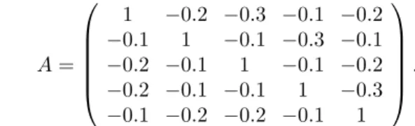
Example 4.2This example is a numerical example intro-duced in [7] and [9]. The coefficient matrixAof (1) is given by:
A=
1 −0.2 −0.3 −0.1 −0.2 −0.1 1 −0.1 −0.3 −0.1 −0.2 −0.1 1 −0.1 −0.2 −0.2 −0.1 −0.1 1 −0.3 −0.1 −0.2 −0.2 −0.1 1
.
parametersw,r, whereρ=ρ(Lr,w),ρ2=ρ(L2,r,w),ρ∗2=
ρ(L∗
2,r,w). All numerical experiments were carried out using Matlab 6.5 with β1 = 1, β2 = 0.1, β3 = 0.2, β4 = 0.1,
β5= 0.3in Table II and β1= 1.1,β2= 1,β3= 1,β4= 1,
β5= 1in Table III, respectively.
TABLE II
SPECTRAL RADII OF THEAORAND PRECONDITIONEDAORITERATION MATRICES
w r ρ ρ2 ρ∗2
1 0 0.6551 0.6480 0.6370
0.2 0.1 0.9288 0.9274 0.9251
0.3 0.2 0.8896 0.8876 0.8839
0.6 0.5 0.7531 0.7495 0.7408
0.6 0.6 0.7423 0.7389 0.7295
0.8 0.7 0.6400 0.6358 0.6223
0.9 0.5 0.6297 0.6242 0.6112
From Tables II-III, it can be seen that ρ∗
2< ρ2< ρwhen
ρ <1. These results are in accordance with the theoretical results in Theorem 3.3 (a).
TABLE III
SPECTRAL RADII OF THEAORAND PRECONDITIONEDAORITERATION MATRICES
w r ρ ρ2 ρ∗2
1 0 0.6551 0.6205 0.6043
0.2 0.1 0.9288 0.9221 0.9187
0.3 0.2 0.8896 0.8798 0.8746
0.6 0.5 0.7531 0.7395 0.7241
0.6 0.6 0.7423 0.7262 0.7139
0.8 0.7 0.6400 0.6203 0.6030
Example 4.3[10] The coefficient matrixAof (1) is given by:
A=
1 q r s q · · ·
s 1 q r . .. q
q s 1 q . .. s
r q s 1 . .. r
s . .. ... ... ... q
· · · s r q s 1
,
where q =−p/n, r =−p/(n+ 1), s =−p/(n+ 2). For
n= 6 andp= 1, Table IV displays the spectral radii of the corresponding iteration matrix with some randomly chosen parametersw,r, whereρ=ρ(Lr,w),ρ1=ρ(L1,r,w),ρ∗1=
ρ(L∗
1,r,w). All numerical experiments were carried out using Matlab 6.5 with α1 = 0.9,α2 = 0.9,α3 = 0.9, α4 = 0.9,
α5= 1.
TABLE IV
SPECTRAL RADII OF THEAORAND PRECONDITIONEDAORITERATION MATRICES
w r ρ ρ1 ρ∗1
0.9 0.8 0.6519 0.5849 0.5773
0.95 0.8 0.6325 0.5618 0.5538
0.8 0.7 0.7083 0.6554 0.6481
0.7 0.65 0.7517 0.7078 0.7012
From Table IV, it can be seen that ρ∗
1 < ρ1 < ρ when
ρ < 1. These numerical results are in accordance with the theoretical results in Theorem 3.2 (a).
V. CONCLUSIONS
In this paper, we proposed three new preconditioners and studied the convergence rates of the new preconditioned AOR methods for solving linear system (1). Comparison results given in Section III show that the new preconditioned AOR methods are better than those proposed by Wang et al. [6], J. H. Yun [8] and A. J. Li [9] whenever these methods are convergent. It can also be seen that all the numerical examples given in Section IV are consistent with the theoretical results given in Section III (Tables I-IV).
It would be nice if we can find optimal values of r and
wfor which the convergence rate of the new preconditioned AOR methods is best. Moreover, by these numerical exam-ples, we found that the relations amongρ¯,ρ∗
1,ρ
∗
2are not only
related to the matrix, but also the seletion of parametersαi,
βi for i= 1,2,· · ·, nin the preconditionersP¯,P1∗ andP
∗
2.
And it is difficult and complicated to find the conditions. Future work will include numerical or theoretical studies for finding the optimal values of r and w and the optimal parameters ofαi,βi for i= 1,2,· · · , n.
ACKNOWLEDGEMENTS
This work is supported by the National Natural Science Foundations of China (No.11171273).
REFERENCES
[1] M. ur Rehman, C. Vuik, and G. Segal, “Preconditioners for the Steady Incompressible Navier-Stokes Problem,”IAENG International Journal of Applied Mathematics, vol. 38, no. 4, pp. 223–232, 2008. [2] O. Kardani, A. V. Lyamin, and K. Krabbenhφft, “A Comparative
Study of Preconditioning Techniques for Large Sparse Systems Arising in Finite Element Limit Analysis,” IAENG International Journal of Applied Mathematics, vol. 43, no. 4, pp. 195–203, 2013.
[3] V. Klement and T. Oberhuber, “Multigrid Method for Linear Comple-mentarity Problem and Its Implementation on GPU,”IAENG Interna-tional Journal of Applied Mathematics, vol. 45, no. 3, pp. 193–197, 2015.
[4] D. W. Deng and T. T. Pan, “A Fourth-order Singly Diagonally Implicit Runge-Kutta Method for Solving One-dimensional Burgers’ Equa-tion,”IAENG International Journal of Applied Mathematics, vol. 45, no. 4, pp. 327–333, 2015.
[5] A. Hadjidimos, “Accelerated overrelaxation method,”Math. Comput., vol. 32, pp. 149–157, 1978.
[6] H. J. Wang and Y. T. Li, “A new preconditioned AOR iterative method for L-matrices,”J. Comput. Appl. Math., vol. 229, pp. 47–53, 2009. [7] A. J. Li, “Improving AOR Iterative Methods For Irreducible
L-matrices,”Engineering Letters, vol. 19, no. 1, pp. 46–49, 2011. [8] J. H. Yun, “Comparison results of the preconditioned AOR methods
for L-matrices,”Appl. Math. Comput., vol. 218, pp. 3399–3413, 2011. [9] A. J. Li, “A New Precoditioned AOR Iterative Method and Compar-ison Theorems for Linear Systems,”IAENG International Journal of Applied Mathematics, vol. 42, no. 3, pp. 161–163, 2012.
[10] S. L. Wu and T. Z. Huang, “A Modify AOR-type Iterative Method for L-matrix Linear System,”ANZIAM J., vol. 49, pp. 281–292, 2007. [11] Y. T. Li, C. X. Li, and S. L. Wu, “Improving AOR method for
consistent linear systems,”Appl. Math. Comput., vol. 186, pp. 379– 388, 2007.
[12] G. B. Wang and N. Zhang, “New preconditioned AOR iterative method for Z-matrices,”J. Appl. Math. Comput., vol. 37, pp. 103–117, 2011. [13] X. Z. Wang, T. Z. Huang, and Y. D. Fu, “Comparison results on preconditioned SOR-type iterative method for Z-matrices linear systems,”J. Comput. Appl. Math., vol. 206, pp. 726–732, 2007. [14] M. Dehghan and M. Hajarian, “Modied AOR iterative methods to
solve linear systems,”Journal of Vibration and Control, vol. 2014, no. 20, pp. 661–669, 2015.
[15] Y. T. Li, C. X. Li, and S. L. Wu, “Improvements of preconditioned AOR iterative method forL-matrices,”J. Comput. Appl. Math., vol. 206, pp. 656–665, 2007.
[17] D. J. Evans, M. M. Martins, and M. E. Trigo, “The AOR iterative method for new preconditioned linear systems,” J. Comput. Appl. Math., vol. 132, pp. 461–466, 2001.
[18] Y. T. Li and S. F. Yang, “A multi-parameters preconditioned AOR iterative method for linear systems,”Appl. Math. Comput., vol. 206, pp. 465–473, 2008.
[19] H. S. Najafi, S. A. Edalatpanah, and A. H. R. Sheikhani, “Convergence Analysis of Modified Iterative Methods to Solve Linear Systems,” Mediterr. J. Math., vol. 11, pp. 1019–1032, 2014.
[20] Q. B. Liu, J. Huang, and S. Z. Zeng, “Convergence analysis of the two preconditioned iterative methods forM-matrix linear systems,”J. Comput. Appl. Math., vol. 281, pp. 49–57, 2015.
[21] H. S. Najafi and S. A. Edalatpanah, “A new of (I+S)-type precondition-er with some applications,”Comp. Math. Appl., pp. 10.1007/s40 314– 014–0161–8, 2014.
[22] R. S. Varga,Matrix Iterative Analysis. Springer, Berlin, 2000. [23] A. Berman and R. J. Plemmoms,Nonnegative Matrices in the
Math-ematical Sciences. SIAM, Philadelphia,PA, 1994.