Second-order plastic-zone analysis of steel frames
Part I: Numerical formulation and examples of validation
Arthur R. Alvarenga and Ricardo A. M. Silveira∗
Department of Civil Engineering, School of Mines Federal University of Ouro Preto (UFOP) Campus Universit´ario
Morro do Cruzeiro, 35400-000 Ouro Preto, MG – Brazil
Abstract
This paper presents a second-order plastic-zone formulation for the non-linear analysis and design of plane steel frames with geometric imperfections and residual stress. The pro-posed numerical methodology has an inelastic formulation based on the plastic-zone method performed by the so-called “slice technique”. This methodology also uses a beam-column finite element model based on the Bernoulli-Euler theory and described in the updated Lagrangian co-rotational system. The considered hypothesis and the adopted kinematic re-lation lead to an element stiffness matrix whose terms represent the constitutive law and second-order effects. An incremental-iterative Newton-Raphson strategy solves the global non-linear equation system and, at the internal force recovery level, in each iteration, an axial-force iterative process is proposed to obtain the axial-force balance at the element ends, more precisely determining the plasticity spread. Three benchmark structural prob-lems are studied and the present work’s findings validate the proposed numerical formulation and the axial-force iterative process. A companion paper discusses in depth the influence of geometrical imperfections and residual stress in steel frame design.
Keywords: Steel frames, Plastic-zone method, Non-linear analysis, Inelastic analysis, Ele-ment axial force
1 Introduction
The effective length K-factor paradox presented by Siat-Moy [28] contributed to a wave of researches showing several conditions under which traditional K-factors could not be precisely defined, failed to give a reasonable answer (over-estimates) or even worse, produced unsafe design.
New solutions or approximations intended to solve the aforementioned drawbacks, as well as others that appear to improve or modify the design process [5, 10, 18]. Giving the AISC point of view prevalent at the time, are works from LeMesurier [22], Hajjar [16], and Hajjar and White [17].
With the application of second-order elastic analysis, it is possible to detect the whole picture of slender structural system. Even in some structural cases, there is no need for the K factor at all (K = 1 [16]). Furthermore, this process is not computer-costly and there is a lot of available software that can perform this kind of analysis. Nevertheless, the main challenge is still to make some sort of second-order analysis by which the K-factor and member check are not obligatory. Research along the last twenty years has brought new ways for the engineer to design without using the old methodology. Computer development paved the way for much research on non-linear methods with both elastic and inelastic approximations. As processor speed, graphic interfaces, software facilities, and memory capacity has expanded, the mathematical formulations and computing programs have grown more complex.
However, only after the publication of Australian Standard AS4100 [1] were designers ex-plicitly allowed to check in-plane member and frame stability solely on a second-order inelastic analysis basis, named hereadvanced analysis. More recently, AISC [25] provided the option for evaluating overall frame stability without effective length factors. To use it, of course, one must know precisely what requirements to obey, so the first step is to define this kind of analysis.
Advanced analysis is a set of accurate second-order inelastic analyses that account for large displacements, plasticity spread and initial imperfection effects. The structural problem is an-alyzed in such a way that the strength or stability limit of the whole (or part of) system is determined precisely, so individual in-plane member checks are not required. It is a direct design.
There are two known research lines to develop a computational advanceddirect analysis in steel framed structures, i.e.:
i. the refined plastic-hinge method, where scalar parameters and tangent modulus account for member rigidity degeneration, which diminishes section properties as soon as yield begins. This method provides good answers and does not require too much computer work [9, 23, 32]. In this context, Chan and Chui [6, 7] proposed a refined plastic-hinge method based on the section assemblage concept [20, 24];
this approach. The Lavall [21] and Pimenta [27] works applied one approximation of this method called slice technique, which the present work also adopts [2, 3].
Besides being considered a complete second-order inelastic analysis, the computational ad-vanced analysis must still fulfill the following minimum requirements:
i. rigorous mathematics formulation based on well-understood engineering theories of solid mechanics;
ii. structural model shall include the stability effects P-∆ and P-δ;
iii. member forces cannot violate the cross section strength: full plasticity condition; iv. structural model must capture plasticity spread;
v. strength, deformations, and internal force distribution must be close to benchmark solu-tions;
vi. initial geometric imperfections and residual stress effects must be included in the analysis. This paper presents a second-order plastic-zone formulation for the non-linear inelastic anal-ysis and design of plane steel frames according to these requirements. Thus, the next section displays the numerical formulation, including the strain field, the finite element model, and the second-order inelastic stiffness matrix. The considered hypothesis and kinematic relations adopted lead to a beam-column element stiffness matrix whose terms represent the constitu-tive law and second-order effects. The standard incremental-iteraconstitu-tive Newton-Raphson strategy solves the global non-linear equation system. This work also presents a new proposal: axial force iterative integration. This iterative process, developed at element level, aims to catch axial force balance when yield starts, which can more closely follow the plasticity spread. To validate this proposed numerical formulation, three steel structures are analyzed and some final remarks are presented in the last section.
A companion paper sheds some light on the last requirement stated above (material and geometric imperfections), called heremain aspects. The initial geometric configurations, treated as a sum of the structure’s out-of-plumbness and some member’s out-of-straightness, coupled (or not), with residual stress effects, are studied on simple and very sensitive structures like portal frames.
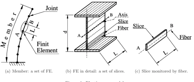
2 The inelastic formulation
Joint
Finit
Element
L
A B
M
e
m
b
e
r
Joint
Finit
Element
L
A B
M
e
m
b
e
r
(a) Member: a set of FE.
Axis Slice Fiber A
B
L
d
Axis Slice Fiber A
B
L
d
(b) FE in detail: a set of slices. A
B
Fiber
Slice
L
A
B
Fiber
Slice
L
(c) Slice monitored by fiber.
Figure 1: Plastic zone model.
The slice’s centerline is namedfiber, as shown in Fig.1(c). The slice technique assumes that, by evaluation of the fiber’s stress-strain relation, it is possible to capture the state of each slice. So integrating the properties of the fiber from all slices along the section will update the section state, with the properties encountered on the two joints. This is similar to the moment-thrust-curvature integration procedure [15]. Hence, this establishes the FE state, giving the plastic-zone formation.
2.1 Strain field and finite element model
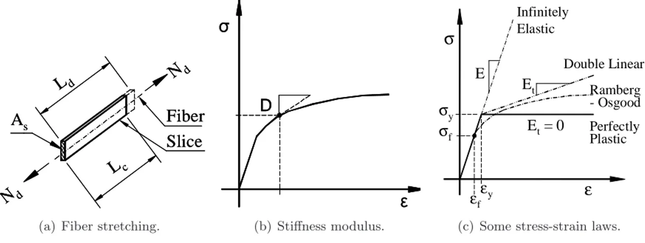
Considering that one fiber in the current state has Lc length, and turns to be Ld length in the deformed (or updated) state, as Fig.2(a) sketches, then the fiber stretchingλand its linear elongation can be defined by:
λ= Ld
Lc
(1a)
ε=λ−1 (1b)
Assuming a fiber to represent the slice as a whole, with slice’s area As, where updated axial forceNddoes fiber stretching, and also knowing the nominal (or Biot) stress σ and linear elongationεenergetically conjugate, the following relations can be written:
σ= Nd
As
(2a)
σ=σ(ε) =Dε, withD= dσ
dε(ε) (2b)
yielding stress of steel; or Et , the tangent modulus, when in the plastic range, σ < σy (see Fig.2(c)). In case of elastic unloading, the stiffness modulus D assumes the value of the Young modulus E.
Applying the plastic-zone method, steel behavior can exhibit some other strain-hardening laws as shown in Fig.2(c). Additionally, to study the member behavior, the following hypotheses are considered:
i. the Bernoulli-Euler simplifications are adopted (all sections remain normal to FE’s axis and cross-sections remain plane after loading application);
ii. the Poisson’s effect is neglected;
iii. all members are braced out-of-plane (the generalized displacements and element forces are in plane only);
iv. the shear stress effect in yielding is disregarded;
v. all cross-sections are compact (WF profiles, which are not recommended for deep sections steel frames);
vi. all members are rigid connected and there is no finite node effect (panel distortion).
Nd
Nd
As
Ld
Lc
Fiber Slice
Nd
Nd
As
Ld
Lc
Fiber Slice
(a) Fiber stretching.
σ
ε D
σ
ε D
(b) Stiffness modulus.
ε σ
εf
εy σf σy
E Et
Et= 0
Infinitely Elastic
Double Linear
Ramberg - Osgood
Perfectly Plastic
ε σ
εf
εy σf σy
E Et
Et= 0
Infinitely Elastic
Double Linear
Ramberg - Osgood
Perfectly Plastic
(c) Some stress-strain laws.
Figure 2: Slice and fiber behavior.
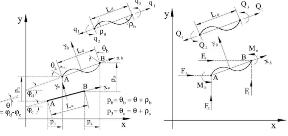
ud(x, yp) =u0d(x)−yp sin ρ (3a)
vd(x, yp) =v0d(x)−yp(1− cosρ) (3b)
in which x is the position of some section along the member (in the local system, in deformed configuration), andyP is the distance between P point and 0 centroid.
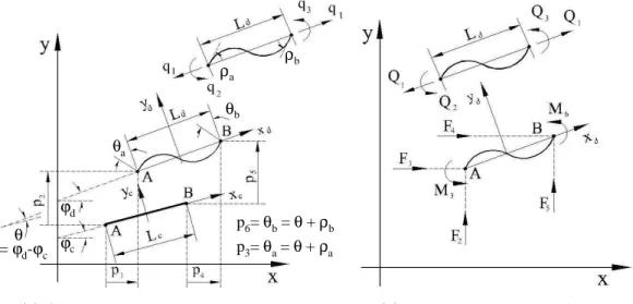
θ ϕd
ϕc
θa
θb
ρb
ρa
p6= θb= θ+ ρb p3= θa= θ+ ρa = ϕd-ϕc
(a) Point P movement related to axis 0. (b) Specific rotation of the fiber.
Figure 3: Fiber and axis relationship.
Figure 3(b) shows a differential FE with length dx, closed by two end sections, where d is the section depth,R0dis the section-axis curvature ratio andRdis the curvature ratio of a fiber placed at generic point P. The elongation of the point P can be written as:
ε=ε0−ypρ′ (4)
in whichε0 is the elongation of the axial fiber and ρ ’ is the angle change of the chord joining
the FE’s ends in relation to the overall parallelx axis.
According to the geometry relations shown in figures, the secant approximation, combining Eqs. (1a) and (1b), and also assuming some simplifications (sinρ∼= tanρ∼=ρ, cosρ∼= 1−ρ2/2
, sec ρ ∼= 1 +ρ2/2 ), the basic relationship for the strain field in the numerical formulation is given by [2, 21, 27]:
ε= (1 +u′0d)
1 +1 2
à v′0d 1 +u′
0d !2
−1−yc v0′′d (1 +u′
0d)
where u0d and v0d are the FE axis’ displacements and yc is the centroid element coordinate which only coincides withyr(reference coordinate, e.g. initial value) in the elastic range. When plasticity begins, the remaining elastic section’s centroid does not necessarily coincide with the EF’s axis, so theyc value has to update for ydat each iteration cycle.
Updated co-rotational Lagrangian formulation evaluates the strain field on the finite element movement. In the local co-rotational system, it defines three displacements as follows (see Fig.4(a)):
q1 =Ld−Lc (6a)
q2=ρa=θa−θ (6b)
q3 =ρb=θb−θ (6c)
where the rotation θ = ϕd−ϕc is the FE’s rigid body rotation, which is subtracted from θa and θb rotations to obtain q2 and q3 , while q1 is the change of EF’s chord length. An overall
Cartesian system of the model describes these nodal motions permitting the conventional three degrees of freedom per node placed together in Fig.4(a), and is written as:
Node A:p1=ua;p2 =va;p3 =θa (7a)
Node B :p4 =ub;p5 =vb;p6=θb (7b)
In the finite element context, u0d and v0d are provided by interpolating functions in the reference configuration. In traditional way, a linear function is chosen foru0dand a third degree polynomial function for v0d :
u0d(x)∼= Ψ1q1 (8a)
vod(x)∼= ·
1 + q1 Lr
¸
[Ψ2q2+ Ψ3q3] (8b)
with
Ψ1(x) =
x
Lr +
1
2 (9a)
Ψ2(x) =
8x3−4Lrx2−2L2rx+L3r 8L2
r
(9b)
Ψ3(x) =
8x3−4Lrx2−2L2rx−L3r 8L2
r
2.2 Second-order inelastic stiffness matrix
Applying the Virtual Work Principle for the FE equilibrium on the reference volumeVr (initial), one can write:
X
i=1 to6
Piδpi = Z
Vr
σδεdVr (10)
As the change of δεcan be expressed using the chain rule (assuming thatεis a function of qα and also qα is related topi ), the following equilibrium relation is obtained:
Pi = Z
Vr
σ µ
∂ε ∂qα
¶ µ ∂qα
∂pi 
dVr=Qα µ
∂qα ∂pi
(11)
beingQαthe co-rotational forces, which correspond to the six Cartesian forces shown in Fig.4(b).
θ ϕd
ϕc
θa
θb
ρb
ρa
p6= θb= θ+ ρb p3= θa= θ+ ρa = ϕd-ϕc
(a) General and co-rotational displacements. (b) Local and co-rotational forces.
Figure 4: Cartesian and co-rotational systems.
Thus, FE’s stiffness matrix refereed to the overall system can be determined by the derivation of Eq. (11) in relation to a global displacementpi . In this way:
Ki,j= ∂Pi ∂pj
=∂qα
∂pi µ
∂Qα ∂qβ
∂qβ ∂pj
+Qα ∂2q
α ∂pi∂pj
= qα,iDα,βqβ,j
| {z }
constitutive law
+ qα,iHα,βqβ,j
| {z }
curvature P−δ
+ Qαqα,ij | {z } P−∆and M−Φ
(12)
where:
Dα,β=
Z
Vr
µ ∂ε ∂qα
¶ D
µ ∂ε ∂qβ
Hα,β = Z
Vr
σ µ
∂2ε ∂qα∂qβ
dVr (13b)
qα,ij = ∂2q
α(ϕd= 0) ∂pi ∂pj
(13c)
The first term represents the constitutive law, while the others include second-order effects caused by FE’s curvature (P-δ) and by both the P-∆ and M-Φ effects. Equation (12) can be rewritten in matrix notation as follows:
K=KM+KH+KGα (14)
where KM is the constitutive stiffness matrix and both KH and KGα define the geometrical stiffness matrix. Numerical approximations provide the components of these matrices, and are given in the Appendix.
Finally, the structure stiffness matrix is built by summing the contribution of every element. As is usual in incremental analyses, some parts of the prescribed nodal loading are applied in steps. This process forms a set of linear equations, which is solved here by Gaussian reduction with backwards substitution [26]. With the displacements known, the stress and strain of every slice from each section (at nodes A or B) can be found and the internal forces evaluated. For the next iteration, the new loading uses the joint forces that were not equilibrated and the cycle stops only when equilibrium of the joint forces is attained (residual forces become negligible). In fact, this is the standard Newton-Raphson iterative strategy to solve nonlinear structural problems [26].
3 Axial force iterative integration (AFII)
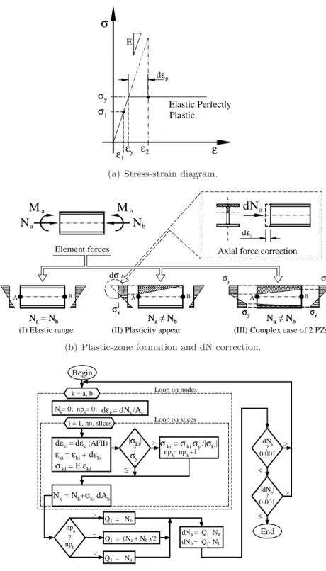
According to Fig.5(a), if some fiber is in the elastic range, for a known strainε1 there is a stress
σ1 < σy , and ε1 =σ1/E < εy . In this case, the internal axial forceQ1 = Nk , with k node index equal to a or b, as shown in Fig 5(b)(I), whereNk is obtained by integrating all slices on side k of FE (see Appendix).
However, when a strain increment occurs like ε2 = ε1 +dε > εy at any load step of an incremental process, the new stress calculated by σ2 =ε1+Edε is greater than σy , therefore
the fiber will be in the plastic range. There will be some plastic strain d p with an elastic strain εy =ε1+dεe in such a way thatε2 =εy+dεp . Figure 5(b)(II), for example, shows a FE where plasticity occurs at node A but the other side remains elastic (node B), and a strip plastic zone will appear along the FE. In this case, the internal axial forceNa6=Nb . This creates a problem about Q1 definition.
E Elastic Perfectly Plastic σ σy σ1 ε1
εy ε2 ε
dεp E Elastic Perfectly Plastic σ σy σ1 ε1
εy ε2 ε
dεp
(a) Stress-strain diagram.
M Na
a
Nb
Mb dNa
A B
A B A B
Element forces Axial force correction
dσ
σy
σy
σy
σy dεa
σy
Na= Nb Na≠ Nb Na≠ Nb
M Na
a
Nb
Mb dNa
A B
A B A B
Element forces Axial force correction
dσ
σy
σy
σy
σy dεa
σy
Na= Nb Na≠ Nb Na≠ Nb
(I) Elastic range (II) Plasticity appear (III) Complex case of 2 PZs
(b) Plastic-zone formation and dN correction.
k = a, b Loop on nodes
Loop on slices i = 1, no. slices
Q = N1 b
Q = N1 a
Q = (N + N )/21 a b
dN = Q - Na 1 a b
dN = Q - Nb 1
< >
=
np = np +1k k
np a
np ?b
|dN |a > 0.001 |dN | 0.001 > b > ? ? ?
N = 0; np = 0;k k
Begin
End dεki = dεk(AFII)
ε
ki =εki+ dεki
σ
ki= E εki
|σki| σki=σki σy/|σki|
Nk= Nk+σkidAki
σ
y
dεk= dNk/Ak
≤ ≤
≤
(c) Simplified flow-chart.
dN =Na−Nb 6= 0 , which cannot be restored with the Newton-Raphson process only. For this reason, the present work proposes a new iterative process to adjust the stress and strain for all FEs with plasticity on any fiber. While the difference|dNk|> tolerance (∼= 0.001 kN) exists, a new axial strain on the node k index (a or b), wheredNk occurs, will be evaluated and is given by:
δεk= dNk
DAck
(15)
in which Ack is the section area in that iteration (current value), obtained at the node k index, that will be updated iteratively. Afterwards, the process finds a new stress, calculates new forces Q, and repeats the whole cycle until convergence. The goal of this procedure is to guarantee that each FE always verifiesQ1 =Na ∼=Nb , assuming the axial force must be constant (fixed between FE extremes). Figure 5(c) shows a simplified flow-chart of this iterative process, which can also solve more complicated cases like that of Fig.5(b)(III).
Moreover, the iterative integration procedure applied here brings the point with plasticity back to the yielding surface, correcting unavoidable distortions from the integrals of forces in plastic zone sections. This procedure is similar to what happens in the refined plastic-hinge approach, where a correction vector is used to keep the point on interaction surface (e.g. when axial force grows, it is necessary to reduce the plastic moment correspondingly [7, 23, 24]).
In the early stages of this formulation and computational program, the co-rotational axial force Q1 was assumed to be a mean value of nodal integrated forces Na and Nb . Using this mean value results in unwanted differences afterwards, and this justifies the present proposal.
4 Examples of validation
Three validation examples are presented. The first investigates a beam-column with member’s out-of-straightness; the second shows the results obtained using the two strategies to evaluate the axial force componentQ1 (with and without the axial force iterative-integration proposed);
and the third, it is the famous Vogel’s portal frame, that is usually adopted for calibrating advanced second-order inelastic analysis.
4.1 Galambos-Ketter’s beam-column
Chenet al. [9] pointed out the structural problem illustrated in Fig.6 as a benchmark problem for second-order inelastic analysis. The goal is to verify the interaction between the axial force and end moments at collapse, for different values of slenderness ratioL/rz , in which L is the column length and rz is the radius of gyration of the cross sectional area surrounding the centroidal axis. Figure 6 also presents the corresponding data, where only the case with no residual stress was considered. A companion paper studies the case with residual stress.
Data:
P = λNy 0 λ 100 %
Steel: ASTM A-36 E = 20000 kN/cm2
σy= 25 kN/cm2
σr= 7.5 kN/cm2
δ0= L/1000
Section: 8 WF 31 Model: 6 FEs L/rz= 60-80-100
MB P MA L B A δ0 Data:
P = λNy 0 λ 100 %
Steel: ASTM A-36 E = 20000 kN/cm2
σy= 25 kN/cm2
σr= 7.5 kN/cm2
δ0= L/1000
Section: 8 WF 31 Model: 6 FEs L/rz= 60-80-100
MB P MA L B A δ0 MB P MA L B A δ0
Figure 6: Galambos and Ketter’s beam-column.
those produced by the BCIN program [9, 11]. The latter also performed a plastic-zone approach but with the finite difference method and using a mesh of 20 sections, having both flange and web divided into 40 strips and an initial out-of-straightnessδ0 = 0.5 mm at the middle length.
This work considered a mesh with only 6 FEs to model the beam-column, and the half-flanges and the web were divided into 20 and 36 slices, respectively.
0 10 20 30 40 50 60 70 80 90 100 M/MP [%]
0 10 20 30 40 50 60 70 80 90 100 N /N y [ % ] .
———Present work
+ + + Chen et al. [9]
L/rz= 60
L/rz= 80
L/rz= 100
N
N M M
Beam-column 8 WF 31 A36
0 10 20 30 40 50 60 70 80 90 100 M/MP [%]
0 10 20 30 40 50 60 70 80 90 100 N /N y [ % ] .
———Present work
+ + + Chen et al. [9]
L/rz= 60
L/rz= 80
L/rz= 100
N
N M M
Beam-column 8 WF 31 A36
N N M M N N M M N N M M Beam-column 8 WF 31 A36
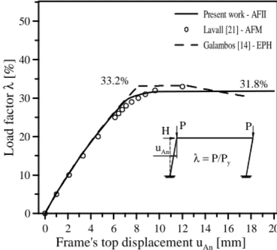
4.2 Galambos’ portal frame
Figure 8 shows the steel portal frame studied by Galambos [14] and also adopted to validate the slices technique formulation [21]. The frame’s equilibrium paths are presented in Fig.9, showing the results obtained by using two different strategies to evaluate the element axial force, i.e., with and without the axial force iterative integration proposed. In the last case, a mean value of the element end axial forces was assumed [21].
L
=
5
0
0
c
m
P
B = 1000 cm
P
H
FE 1
1
2 12 FE 12
13
Data:
P = 1883 kN H = 188.3 kN Steel: ASTM A 441 E = 20500 kN/cm2 σy= 35 kN/cm2
Columns: HPL 240 Beam: HPL 200 Model: 4 FEs by member Load factor: 0 ≤ λ ≤ 40 %
L
=
5
0
0
c
m
P
B = 1000 cm
P
H
FE 1
1
2 12 FE 12
13
Data:
P = 1883 kN H = 188.3 kN Steel: ASTM A 441 E = 20500 kN/cm2 σy= 35 kN/cm2
Columns: HPL 240 Beam: HPL 200 Model: 4 FEs by member Load factor: 0 ≤ λ ≤ 40 %
Figure 8: Galambos’ portal frame equilibrium path.
The equilibrium paths computed by theaxial force iterative integration(AFII) andaxial force mean(AFM) are very close to the answers by Galambos as displayed in Fig.9. The collapse loads, presented in Tab. 1 with the driftuAnprior collapse, show close agreement as well. Nevertheless, it is worth mentioning that when the structural collapse is caused by inelastic buckling instead of incomplete plastic mechanism formation, the numerically determined collapse load by the AFM strategy tends to be a little bigger and the equilibrium path increases a little, too. Figure 9 illustrates this behavior.
Table 2 shows the internal forces near collapse load on elements 1 and 12 obtained by AFII and AFM. While the first has the same value for axial forces (Na∼=Nb ) the latter has different ones (Na < Nb ). In this example, plasticity only happens at node A, while node B remains elastic at that selected FE. This drawback can only be detected when the integrated axial forces are printed. Moreover, Tab. 2 shows that not only the Na and Nb values are different when using AFM, but also the bending moments in the plastic-zone nodes (1 and 12) are bigger than expected. In contrast, on the other end (2 and 11 nodes), forces continue to grow reaching plasticity. Briefly: the axial force begins to reduce in node A and to grow at node B as the Newton-Raphson iterations develop and the moment is not reduced in those plastic zones as would be expected!
0 2 4 6 8 10 12 14 16 18 20
Frame's top displacement uAn [mm]
0 10 20 30 40 50
L
o
ad
f
ac
to
r
λ
[%
]
Present work - AFII Lavall [21] - AFM Galambos [14] - EPH
λ = P/Py
uAn
H P P
33.2% 31.8%
Figure 9: Galambos’ portal frame.
Table 1: Galambos’ frame: collapse load factor and drift.
Galambos [14] Lavall [21] Present Work
EPH(4) PZ PZ
λ[%] uAn [cm] λ[%] uAn [cm] λ[%] uAn [cm]
31 7.464 31.0 8.769 31 8.378
32 7.780 32.0 9.615 31.7 9.965
33.2 8.167 33.0 12.006 31.8(3) 33.633
30.47(1) 17.50 34.0(2) - -
-Notes: 1. Galambos does not define collapse-load; 2. No further information;
3. Matrix shows singularity, last iteration’s driftuAnis given;
4. EPH: second-order elastic-plastic hinge.
Table 2: Galambos’ frame: forces near collapse.
λ(1) FE
Node(2) AFM: Axial Force Mean(6) AFII: Axial Force
[%]
Iterative Integration
A B Na Nb Ma Mb dN(3) Q
(4)
1 Na=Nb Ma Mb
[kN] [kN] [kNcm] [kNcm] [kN] [kN] [kN] [kNcm] [kNcm]
30 1 1 2 543.426 553.649 10244.0 6156.9 -10.223 548.538 548.505 10254.7 6161.0 12 12 13 573.641 587.978 6090.5 10114.3 14.337 580.810 580.840 6075.6 10100.0
31 1 1 2 555.816 575.879 10681.3 6340.0 -20.063 565.848 565.657 10684.3 6319.3 12 12 13 588.273 613.813 6231.0 10490.1 25.540 601.043 601.214 6194.0 10471.2
Notes: 1. The collapse occurs atλ= 31.8;
2. Plasticity appear at nodes 1 and 13 only, while nodes 2 and 12 remain elastic; 3. dN=Na−Nb; 4. Q1= (Na+Nb)/2
the absolute value of dN ≥ 0.001 kN or when a given number of cycles (200 adopted here) are performed without convergence.
4.3 Vogel’s portal frame
Figure 10 [31] shows this portal frame and all required data. The European rolled shapes were used considering ECCS [12], with a residual stress of σr = 0.5 σy . Furthermore, the structural model, as required by advanced analysis, includes the out-of-plumbness ∆0 = L/400 and the
out-of-straightness σ0 = L/1000 for both columns. Since the frame collapse is determined
by the column’s inelastic buckling, this example is a good benchmark test for any inelastic formulation [11].
B = 400 cm
L
=
5
0
0
c
m
H
P P
0.5 cm 1.25 cm
0.5 cm
Data:
P = 2800 kN H = 35 kN Steel: ASTM A-7 E = 20500 kN/cm2
σy= 25 kN/cm2σr= 11.75 kN/cm2
Colums: HEB 300 with 8 FEs Beam: HEA 340 with 6 FEs
δ0= L / 1000 ∆0= L / 400
Load factor: 0 ≤ λ ≤ 105 %
B = 400 cm
L
=
5
0
0
c
m
H
P P
0.5 cm 1.25 cm
0.5 cm
Data:
P = 2800 kN H = 35 kN Steel: ASTM A-7 E = 20500 kN/cm2
σy= 25 kN/cm2σr= 11.75 kN/cm2
Colums: HEB 300 with 8 FEs Beam: HEA 340 with 6 FEs
δ0= L / 1000 ∆0= L / 400
Load factor: 0 ≤ λ ≤ 105 %
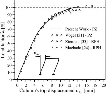
Figure 10: Vogel’s portal frame.
Ziemian et al. [33] and Clarke [11], both applying PZ formulation, adopted 120 elements (50 FEs by column). Based on plastic-hinge methodology, Teh and Clarke [29] and Machado [24] used four FEs for the whole structure. There is not much details about Liew’s FE model, who used the refined plastic-hinge and notional load approaches [9]. Avery and Mahedran [4], and Kim and Lee [19], using the Abacus commercial software, modeled the frame with 8952 3D-shell elements. Chan and Zhou [8] adopted the coarsest mesh (one FE by member) and the refined plastic-hinge method with a high-order polynomial function called PEP.
Table 3 displays the collapse load factor λcol and the column top horizontal displacement uAn . This table shows that displacements ranging from 14.2 to 17.3 mm are a good response and the present work’s value falls within this range.
Table 3: Vogel’s frame: collapse load factor and drift
Collapse Vogel Ziemian Clarke Chen et al.
point [31] [33] [11] [9]
PZ EPH PZ RPH PZ NL-PH RPH
λcol [%] 102.2 101.7 99.9 105.0 102.3 99.9 96.0
uAn [mm] 17.3 11.5 14.2 12.0 17.1 12.9 14.8
Collapse Teh and Avery and Kim and Chan and Machado Present
point Clarke [29] Ma-hendran [4] Lee [19] Zhou [8] [24] Work
PZ PZ PZ PEP RPH AS-PH PZ
λcol [%] 100.5 101.0 103.0 103.3 94.0 98.0 100.7
uAn [mm] 20.0 16.2 19.2 16.0 17.01 32.56 17.00
Notes on methods: PZ - plastic zone; EPH - second-order elastic-plastic hinge;
RPH - refined plastic hinge; NL-PH - notional load plastic hinge;
PEP - polynomial enhanced plastic hinge; AS-PH - assembly section plastic hinge [6]
collapse load, in which N is the axial force, Q the horizontal shear, and M the bending moment. The subscript letters mean: (A) left column, (B) beam and (C) right column, (1) base node and (n) columns top node. The present work’s values are again near Vogel’s and Ziemian’s, both with PZ formulation, and show a slight difference in relation to the other researchers’ answers.
0 2 4 6 8 10 12 14 16 18 20
Column's top displacement uAn [mm]
0 10 20 30 40 50 60 70 80 90 100
L
o
ad
f
ac
to
r
λ
[%
]
Present Work - PZ Vogel [31] - PZ Ziemian [33] - RPH Machado [24] - RPH uAn
Figure 11: Vogel portal frame’s equilibrium path.
Table 4: Vogel’s frame: forces near collapse.
Forces(1)
Vogel Ziemian Clarke Chenet al. Machado Present
[31] [33] [11] [9] [24] Work
PZ PZ PZ RPH NL-PH AS-PH PZ
NA
[kN]
2770.2 2765.0 2821.0 2649.0 2752.0 2711.0 2780.7
NC 2829.9 2843.0 2905.0 2721.0 2846.0 2791.0 2858.5
NB 13.4 - - - 15.8
Q1 30.8 - - - 40.5
Qn 28.4 - - - 21.7
MA1
[kNcm]
9071.0 8703.0 9385.0 8586.0 10600.0 9248.0 9854.4
MAn 7464.0 7955.0 8721.0 7357.0 9580.0 8174.0 8058.1
MC1 9055.0 8242.0 8277.0 8389.0 9270.0 8784.0 8832.1
MCn 7462.0 7573.0 8084.0 7069.0 9207.0 7804.0 7492.7
λcol 1.022 0.999 1.023 0.960 1.040 0.980 1.007
FE/col. - 50 50 1 1 1 8
Notes: 1. Indexes: A and C for left and right column, B for beam, 1 and n for first and last nodes in the member;
2. some values are not given in the existing literature.
created by compression along the member, and no yielding occurs in the beam. These two columns’ plastic-zones seem to be equal, and the collapse happens by inelastic instability.
36.7
0 56.0
10.8
6.4 44.7
39.1 7.1
Plasticity[%] : compression FE’s center line
λ = 100.7 %
36.7
0 56.0
10.8
6.4 44.7
39.1 7.1
Plasticity[%] : compression FE’s center line
λ = 100.7 %
5 Final remarks
A numerical procedure involving a second-order inelastic analysis of steel structures using the plastic-zone method and producing a new axial force iterative integration procedure is presented in this paper. The slice technique is the base for the plastic-zone formulation adopted. All three studied benchmark problems presented good agreement with those found in literature. This seems to validate the proposed formulation.
It is worth noting that the proposed numerical methodology was able to trace what occurs inside the steel section and along the member, which means the identification of the start and spread of plasticity. Therefore, this formulation can supply a more comprehensive investigation on the strength and stability of the steel structures.
Based on the nonlinear analysis carried out here and other already-solved steel frame prob-lems, when comparing the proposed numerical methodology with other formulations or methods, the following comments can be made:
i. the quality and precision of the obtained responses are equivalent to those obtained from Abaqus or Ansys 3D plastic zone solutions, even using a more simplified model;
ii. once considered as one more precise numerical formulation, our responses can be used to validate refined plastic-hinge computational implementations, which naturally have dif-ficulties with plasticity spread simulation but do not require too much computer work; and
iii. when compared with others plastic zone approaches, the proposed axial force iterative inte-gration maintains the quality of the internal force recovery, more precisely determining the plasticity spread and for this reason a better answer is obtained.
These comments justify and even make attractive the development of this line of research. In spite of this, it should be mentioned that there is a long road ahead in making this process available for offices. For example, some cases of load increment strategies can lead the solution toward stationary points, among other critical points. In seeking completeness, this method also deserves improvement to fulfill the design needs of non-linear connection behavior, as well as 3D analysis.
6 Acknowledgments
The authors are grateful for the financial support from the Brazilian National Council for Scien-tific and Technological Development (CNPq/MCT), CAPES and the Minas Gerais Research Foundation (FAPEMIG). They also acknowledge the support from the Brazilian Steel Company USIMINAS for this research. Special thanks go to Professor Michael D. Engelhard from Univer-sity of Texas at Austin for his valuable suggestions; and John White and Harriet Reis for their editorial reviews.
References
[1] AS 4100. Steel structures. Standards Association of Australia, Sidney, Australia, 1990.
[2] A.R. Alvarenga. Main aspects in plastic-zone advanced analysis of steel portal frames. M.Sc. thesis, Civil Engineering Program, EM/UFOP, Ouro Preto, MG, Brazil, 2005. (in Portuguese).
[3] A.R. Alvarenga and R.A.M. Silveira, editors. Considerations on Advanced Analysis of Steel Por-tal Frames, Proceedings of ECCM III European Conference on Computational Mechanics Solids, Structures and Coupled Problems in Engineering, Lisbon, Portugal, 2006. pp 2119.
[4] P. Avery and M. Mahendran. Distributed plasticity analysis of steel frame structures comprising non-compact sections. Engineering Structures, 22:901–919, 2000.
[5] R. Bjorhovde. Effect of end-restraint on column strength – practical applications.AISC Engineering Journal, 1:1–13, 1984.
[6] S.L. Chan and P.P.T. Chui. A generalized design-based elastoplastic analysis of steel frames by section assemblage concept. Engineering Structures, 19(8):628–636, 1997.
[7] S.L. Chan and P.P.T. Chui. Nonlinear static and cyclic analysis of steel frames with semi-rigid connections. Elsevier, Oxford, 2000.
[8] S.L. Chan and Z.H. Zhou. Elastoplastic and large deflection analysis of steel frames by one element per member, ii: Three hinges along member. Journal of Structural Engineering ASCE, 130(4):545– 553, 2004.
[9] W.F. Chen, Y. Goto, and J.Y.R. Liew. Stability design of semi-rigid frames. John Willey and Sons, New York, 1996.
[10] W.F. Chen and E.M. Lui. Structural stability – theory and implementation. Elsevier, New York, 1987.
[11] M.J. Clarke. Plastic zone analysis of frames. In W.F. Chen and S. Toma, editors,Advanced analysis of steel frames: theory, software and applications. CRC Press, Boca Raton, 1994.
[12] ECCS. Ultimate limit state calculations of sway frame with rigid joints. Technical working group 8.2, publication 33, European Convention for Constructional Steelwork, Brussels, 1984.
[14] T.V. Galambos.Structural Members and Frames. Dept. Civil Engineering, Un. Minnesota Mineapo-lis, 1982.
[15] T.V. Galambos and R.L. Ketter. Columns under combined bending and thrust. Transations ASCE, 126(1):1–25, 1961. New York, 1959.
[16] J.F. Hajjar. Effective length and notional load approaches for assessing frame stability: Implications for American steel design, Task Committee on Effective Length of the Technical Committee on Load and Resistance Factor Design of the Technical Division of the Structural Engineering. Institute of the American Society of Civil Engineers, Reston, Va., 1997.
[17] J.F. Hajjar and D.W. White. Stability of steel frames: the cases for simple elastic and rigorous inelastic analysis - design procedure. Engineering Structures, 22:155–167, 2000.
[18] S.E. Kim, M.K. Kim, and W.F. Chen. Improved refined plastic hinge analysis accounting for strain reversal. Engineering Structures, 22:15–25, 2000.
[19] S.E. Kim and D.H. Lee. Second-order distributed plasticity analysis of space steel frames. Engineer-ing Structures, 24:735–744, 2002.
[20] A. Landesmann. Analysis and implementation of plastic model for steel framed structures. M.Sc. thesis, Civil Engineering Program/COPPE/UFRJ, Rio de Janeiro, RJ, Brazil, 1999. (in Portuguese).
[21] A.C.C. Lavall. A consistent theory formulation for non-linear analysis by finite element method considering initial imperfections and residual stress in cross section. D.Sc. Dissertation, EESC/USP, S˜ao Carlos, SP, Brazil, 1996. (in Portuguese).
[22] W.J. LeMesurier, editor. Simplified K-factors for stiffness controlled designs, 1797-1812, New York, 1995.
[23] J.Y.R. Liew, D.W. White, and W.F. Chen. Second-order refined plastic-hinge analysis for frame design. parts i and ii. Journal of Structural Engineering, ASCE, 119(11):3196–3237, 1993.
[24] F.C.S. Machado. Second-order inelastic analysis of steel structured systems. M.Sc. thesis, Civil Engineering Program EM/UFOP, Ouro Preto, MG, Brazil, 2005. (in Portuguese).
[25] American Institute of Steel Construction. Specification for structural steel buildings. AISC, Chicago, 2005.
[26] D.R.J. Owen and E. Hinton.Finite elements in plasticity: theory and practice. Pineridge Press Ltd, Swansea, UK, 1980.
[27] R.J. Pimenta. Proposition of buckling curve for welded wf built from fire cut plates. M.Sc. thesis, Federal University of Minas Gerais, Belo Horizonte, MG, Brazil, 1996. (in Portuguese).
[28] F.C. Siat-Moy. K-factor paradox. Journal of Structural Engineering ASCE, 112(8):1747–1760, 1986.
[29] L.H. Teh and M.J. Clarke. Plastic-zone analysis of 3d steel frames using beam elements. Journal of Structural Engineering ASCE, 125(11):1328–1337, 1999.
[30] S. Vinnakota and C.M. Foley. Inelastic behavior of multistory partially restrained steel frames. parts i and ii. Journal of Structural Engineering ASCE, 125(8):854–868, 1999.
[32] R.D. Ziemian and W. McGuire. Modified tangent modulus approach, a contribution to plastic hinge analysis. Journal of Structural Engineering ASCE, 128(10):1301–1307, 2001.
[33] R.D. Ziemian, W. McGuire, and G.G. Deierlein. Inelastic limit state design, part i: Planar frames studies; part ii: Three-dimensional frame study. Journal of Structural Engineering ASCE, 118(9):2352–2568, 1992.
Appendix: The finite element matrices and numerical integration
KM =
D1m
Lr 0
D2m
Lr −
D1m
Lr 0
D2m
Lr
12D3m
LrL2d
6D3m
(LrLd) 0 −
12D3m
(LrL2d)
6D3m
(LrLd)
4D3m
Lr
D2m
Lr −
6D3m
(LrLd)
2D3m
Lr
D1m
Lr 0 −
D2m
Lr
12D3m
(LrL2d) −
6D3m
(LrLd)
sim. 4D3m
Lr (16)
KH =
0 0 0 0 0 0
Q1
5Ld
Q1
10 0 −
Q1
5Ld
Q1
10
2Q1Ld
15 0 − 2Q1
15 −
Q1Ld
30
0 0 0
Q1
5Ld −
Q1
10
sim. 2Q1Ld
KGα =
0 Q2L+2Q3
d
0 0 −Q2L+2Q3
d
0
Q1
Ld 0 −
Q2+Q3 L2
d
−Q1Ld 0
0 0 0 0
0 Q2L+2Q3
d
0
Q1 Ld 0
sim. 0 (18)
The FE matrices have terms related to deformed length (Ld), which changes at each iterative step, and also to initial or reference length (Lr), which is fixed from the beginning of the analysis. Besides the co-rotational forcesQ1 ,Q2 and Q3 , there are the termsD1m ,D2m and D3m that represent the elastic-plastic geometrical properties of the section to be evaluated at each step of the incremental-iterative process. These geometrical properties are obtained by average values using:
Djm = 0.5(Dja+Djb), withj= 1,2,3 (19)
whereDjk is evaluated at the k node index (a or b) as follows:
Djk = Z
Ar
D(yc)(j−1)dAr=
no. slices X
i=1
h
Di(yci)(j−1)dArii (20)
in whichD1k,D2k andD3kare evaluated numerically by DdA,DycdAandDyc2dAintegration, respectively.
The co-rotational axial force on FE is defined by the new process proposed: Q1 = AFII
(Na, Nb ), where AFII is the Axial Force Iterative Integration applied to the axial forcesNa and Nb obtained from integration on k node index (a or b), respectively, using the expression:
Nk=
Z Ar σdAr= no. slices X i=1
[σi dAri] (21)
in such way that these integrals have the same value asQ1 .
The co-rotational moments Q2 = -Ma andQ3 =Mb , are also given by:
Mk =
Z
Ar
σycdAr =
no. slices X
i=1
![Figure 8 shows the steel portal frame studied by Galambos [14] and also adopted to validate the slices technique formulation [21]](https://thumb-eu.123doks.com/thumbv2/123dok_br/15701199.629101/13.892.174.683.319.561/figure-portal-studied-galambos-adopted-validate-technique-formulation.webp)
![Figure 10 [31] shows this portal frame and all required data. The European rolled shapes were used considering ECCS [12], with a residual stress of σ r = 0.5 σ y](https://thumb-eu.123doks.com/thumbv2/123dok_br/15701199.629101/15.892.171.681.405.695/figure-portal-required-european-rolled-shapes-considering-residual.webp)