Constructing efﬁcient substructure-based preconditioners for BEM systems of equations

(1)

Constructing efﬁcient substructure-based preconditioners

for BEM systems of equations

$

F.C. de Arau´jo

a,n

, E.F. d’Azevedo

b

, L.J. Gray

b a_{Department of Civil Eng., UFOP, 35400-000 Ouro Preto-MG, Brazil} b_{Computer Science and Math. Div., ORNL, Oak Ridge, P.O. Box 2008, USA}

a r t i c l e

i n f o

Article history:

Received 11 March 2010 Accepted 13 August 2010 Available online 14 October 2010

Keywords:

3D boundary-element models Subregion-by-subregion algorithm Krylov solvers

Substructure-based block-diagonal preconditioners

a b s t r a c t

In this work, a generic substructuring algorithm is employed to construct global block-diagonal preconditioners for BEM systems of equations. In this strategy, the allowable fill-in positions are those on-diagonal block matrices corresponding to each BE subregion. As these subsystems are independently assembled, the preconditioner for a particular BE model, after theLUdecomposition of all subsystem matrices, is easily formed. So as to highlight the efficiency of the preconditioning proposed, the Bi-CG solver, which presents a quite erratic convergence behavior, is considered. In the particular applications of this paper, 3D representative volume elements (RVEs) of carbon-nanotube (CNT) composites are analyzed. The models contain up to several tens of thousands of degrees of freedom. The efficiency and relevance of the preconditioning technique is also discussed in the context of developing general (parallel) BE codes.

1. Introduction

Applying iterative solvers to large-order engineering problems has been intensively pursued in the last decades, mainly because

their unquestionable appeal to solve truly large models [1,2].

Herein, the parallelism embedded in them allied with the today’s parallel computer architectures plays a decisive role, so that it can be well stated that developing fast scalable (preconditioned) parallel Krylov solvers is a key point for getting high-ﬁdelity solution for large-order complex engineering problems. In these cases, direct solvers may be exceedingly expensive concerning both memory and CPU time, and their parallel implementation is awkward.

For general non-symmetric matrices, like BE matrices, based on the number of terms involved in the iterative formulas, the Krylov solvers can be subdivided in two broad classes of algorithms: long-recurrence algorithms (GMRES and variants) and short-recurrence ones (Bi-CG and variants). Over the last several decades, milestone contributions in these algorithms have been deﬁnitely given by the following works: the Lanczos method

(by Lanczos in 1952)[3], the Bi-CG method (by Fletcher in 1976)

[4], the GMRES method (by Saad and Schultz in 1986)[5], the CGS

method (by Sonneveld in 1989)[6], the Bi-CGSTAB (by van der Vosrt

in 1992)[7], and the Bi-CGSTAB(l) (by Sleijpen and Fokkema in

1993)[8]. Of course, in this period of time, a series of other works

that significantly contributed for increasing the efficiency of Krylov solvers have also been published, including those related to particular applications to symmetric definite matrices.

Particularly for BEM systems of equations, the ﬁrst successful applications of iterative solvers were reported at the end of the

80s and beginning of the 90s[9–12], wherein

diagonal-precondi-tioned Bi-CG[9–10,12], and preconditioned GMRES[11]methods

were used. According to the authors’ knowledge, before these works, only basic iterative methods as the Jacobi or Gauss–Seidel methods, or at most the CGN solver, which consists of applying

the CG method to the normal equations, ATAx¼ATb, had been

considered [13–14]. A patent disadvantage of these iterative

solvers are the non-reliability regarding convergence, so that they actually cannot be regarded as general-purpose solvers for practical applications. In fact, applying basic iterative methods, convergence is assured only if the spectral radius of the corresponding iteration matrix is less than 1, which is not the case for general systems. On the other hand, considering the CGN has the disadvantage of squaring the condition number of the

original systemAx¼b, which may cause the iterative process fail

to converge. The Bi-CG and GMRES methods, and their variants (or combinations) are then the remaining alternatives for deriving general-purpose solvers for BEM equations.

In fact, long-term recurrence methods as GMRES and variants should be avoided because of memory requirements for large problems and non-rare convergence stagnation in practice.

Contents lists available atScienceDirect

journal homepage:www.elsevier.com/locate/enganabound

Engineering Analysis with Boundary Elements

$

Sponsors: Brazilian Research Council, CNPq; Research Foundation of the State of Minas Gerais, FAPEMIG; Ofﬁce of Advanced Scientiﬁc Computing Research, U.S. Department of Energy.

n

Corresponding author. Tel.: +55 31 3559 1468; fax: +55 31 3559 1548.

(2)

Restarting the iterative process after a numbermof iterations is an obvious strategy for reducing memory costs involved in using

GMRES, but, depending on the choice of m, bad convergence

characteristics (including stagnation) may be enhanced, also leading to non-reliable solvers for general purposes in practice. Concerning the Bi-CG method, the shortcoming is its erratic convergence behavior. Thus, a likely optimal iterative solver should be generated by combining the Bi-CG method, which takes into account short-term recurrences, with a residual-minimization method, as the GMRES, which should smooth out convergence irregularities connected with the Bi-CG iterations. Following these

ideas culminated in developing the transpose-free Bi-CGSTAB(l)

[8]and the GPBi-CG (generalized product Bi-CG)[15]solvers.

Whether or not solvers like the Bi-CGSTAB(l) or the GPBi-CG

will always, sure and fast, provide an accurate solution for any practical problem, it is a question that does not have any mathematically founded answer yet. However, two facts are relevant herein. First, convergence failure or slowness is a token that the corresponding model is not suitable for the description of the physical response; second, preconditioners may be employed

to accelerate the iterative process[1,17]. For BEM solvers, a series

of preconditioners have been reported in the technical literature

[9–12,16–19,20]. In general, the splitting matrix of basic iterative methods as the Jacobi, block Jacobi, Gauss–Seidel or incomplete

LUdecomposition methods can be used to construct

precondi-tioners. Roughly speaking, preconditioners are also a way to state a relationship between direct and iterative solvers, in the sense that if the preconditioning matrix becomes the system matrix, so the iterative method at hand becomes a direct solver (giving then the system solution at one single iteration step). Furthermore, domain decomposition methods (DDM) allied with direct meth-ods may also be employed to construct global preconditioners. Herein, in general, direct solvers are employed to get the solution for the many subdomains, while iterative techniques describe the interactions between them. Concerning the parallel processing (actually not addressed in this study), we see that domain decomposition strategies also suits to easily parallelize incomplete

LU-based preconditioners, indeed the most efﬁcient ones, but not

easily parallelizable. In case of block-diagonal preconditioners, the parallelization is straightforward. Thus, DDM-based precondi-tioners are very convenient for developing parallel solvers.

In this work, we objectively employ the BE substructuring

algorithm[21–22]to form a global block-diagonal preconditioner.

This substructuring algorithm is nothing other than a DDM-based strategy to decompose a certain problem domain into a generic number of coupled BE models, so that the preconditioning here developed can be designated as a BE-subdomain-based precondi-tioner. Although the coupling conditions between the subdomains are imposed in a direct (non-iterative) way, the subsystems are independently assembled, and so the block-diagonal matrices corresponding to each subregion can be easily decomposed in

theirLandUfactors. It is worth commenting that the price paid

for constructing this preconditioning, which is much higher than e.g. a plain diagonal one, is in fact insigniﬁcant if convergence reliability and convenience for developing general parallel boundary-element codes is attained. Moreover, the more the number of subregions, the less expensive the constructing of the BE-substructuring-based preconditioner is. For the applications here, the preconditioning proposed is incorporated into the Bi-CG solver. As this solver is theoretically less efﬁcient than the

Bi-CGSTAB(l) or the GPBi-CG solvers, as discussed above, the

efﬁciency of the preconditioner itself will be highlighted in the numerical experiments.

This paper is structured in the following way: we present an overview of the generic BE substructuring algorithm in Section 2, the construction of the preconditioner in Section 3, and analyze

different complex carbon-nanotube (CNT) composites in Section 4. The models considered contains up to several tens of thousands of degrees of freedom. The efﬁciency and relevance of the pre-conditioning proposed is discussed also in the context of ideas for developing general scalable BE parallel codes, in effect the goal of the chief ideas on the base of this paper.

2. The boundary-element substructuring algorithm

The fact that the boundary element method (BEM) is derived from the exact boundary-integral representation of problem solutions, in closed or open domains, accounts for the following advantages: high accuracy, fulﬁllment of radiation conditions in open domains, and easier mesh generation. Indeed, very accurate responses are obtained if homogeneous single-domain problems are considered and the integrals involved are accurately evaluated. However, this is way not the case in practice, wherein e.g. material heterogeneity is often present, and a BE subregion technique is in general needed. Here, the BE subregion-by-subregion (BE-SBS) algorithm reported in

Refs. [21,22] is adopted to both model complex heterogeneous

problems as CNT composites, and to construct preconditioners to be used together with the Krylov solver embedded.

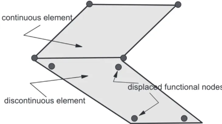
To derive the BE-SBS algorithm, besides continuous elements, discontinuous boundary elements are employed when needed. Herein, another interesting characteristic of the BEM is taken into account: interelement compatibility (in the FE sense) is not required to assure solution convergence. Actually, discontinuous elements allow generating very complex boundary-element models, for instance containing a number of inclusions and voids as in composites. If only continuous boundary elements were used, setting up complex coupled models for general problems

may be awkward[23]. Thus, considering discontinuous boundary

elements is very convenient. However, because of the unavoidable proximity of the displaced collocation (functional) nodes to

neighboring elements (seeFig. 1), besides singular, nearly singular

integrals also take place, and special quadratures are required. As known, in 3D elasticity standard boundary-element formulations, surface integrals of the form

Z

Ge p

Ge u

ikandpikare the Kelvin fundamental kernels,ui

andpithe boundary displacement and traction, respectively, and

G

e the surface of the eth boundary. Actually, the efﬁcient

evaluation of these integrals in the singular and nearly singular

continuous element

discontinuous element

displaced functional nodes

(3)

cases is needed for getting high-quality responses. In previous

works [21,22,24–28], several numerical quadratures have been

investigated. One has concluded that the numerical integration

strategy proposed in Ref. [22] was the best one among the

techniques observed. It has the following characteristics:

1. Weakly singular and nearly weakly singular surface integrals

are computed by combining triangle-polar [24]and

polyno-mial coordinate transformations[25];

2. Nearly strongly singular integrals are evaluated by applying

the line-integral approach reported in Refs.[26,27] together

with the improvements brought about in Ref. [22], which

concern the inclusion of analytical expressions for nearly strongly singular line integrals occurring in the process.

3. Strongly singular integrals (Cauchy principal values) are indirectly calculated by applying rigid-body displacements.

In the above, the termsnearly weakly singularandnearly strongly

singular integrals mean a nearly singular integral associated,

respectively, with u

ik (the weakly singular kernel) and pik (the

strongly singular kernel). All details of the quadratures involved are

described in Ref.[22]. Of course, this integration strategy also suits

to model thin-walled domains, allowing then e.g. the modeling of shell-like elements by means of 3D formulations.

With proper integration procedures, discontinuous boundary elements can be used, and so the BE-SBS algorithm, reported in

Refs.[21,22], is derived. This algorithm is comparable to the

element-by-element (EBE) technique, developed to ﬁnite-element analysis

(4)

(FEA)[29]while a subregion or substructure corresponds to a finite element. Notice that, if needed, we could have a subregion mesh as fine as a finite-element mesh, and if the BE global system matrix were explicitly assembled, it would be highly sparse as well. Furthermore, the BE-SBS algorithm can also be compared to finite

element tearing and interconnecting (FETI) methods[30], where a

given problem domain is decomposed (torn) into non-overlapping subdomains and posteriorly interconnected by imposing the corresponding continuity conditions at the interfaces.

Unlike other BE–BE coupling algorithms which look for suitable compressed formats to store the corresponding global

sparse matrix[31,32], the main idea of the BE-SBS method, which

takes into account Krylov iterative solvers, is to get the global response for a problem working exclusively with its local full-populated subsystems of equations, which are independently generated and stored. No global explicit system matrix is assembled; no zero blocks are stored or handled. The boundary

conditions for the ith subdomain (associated with the outer

boundary of

Oi

, denoted by

Gii

) are introduced during the matrix

assembly for each subsystem. The interface conditions, e.g. at the

interface

Gij

(between the subdomainsiandj), given by

uij¼uji pij¼ pji at

G

ij (

ð2Þ

are directly (not iteratively) imposed while calculating the matrix–

vector products during the iterative solution process, whereuijandpij

denote, respectively, the displacement and traction vectors of

sub-domainiat

Gij

. Thus, fornssubregions, after introducing the boundary

conditions, the BE global system of equations is then given by

X

i1

m¼1

ðHimumiGimpimÞ þAiixiþ

X

ns

m¼iþ1

ðHimuimþGimpmiÞ ¼Biiyi,i¼1,ns,

ð3Þ

whereAii,Bii,HijandGijdenote the regular BE matrices obtained for

source points pertaining to subregion

Oi

and associated, respectively,

with the boundary vectorsxi,yi,uijandpij. Note thatxiandyiare the

vectors containing the boundary unknown and boundary prescribed

values of

Oi

(after column interchange).

To accelerate the solver iterations, structured matrix–vector

products (SMVP) [21,28] are employed. Herein, the matrix

columns of a given subregion are grouped into three separate

blocks: one associated with interfaces

Gij

for which i4j, a

second associated with the outer boundary

Gii

, at which boundary

values are prescribed, and one associated with interfaces

Gij

for ioj. This corresponds to the matrix structuring given

in (4) below

]

[

]

[

1 , 1 , 1 1 , 1 , 1 in i i ii i i i i in i i ii i i i i

G

B

G

H

A

H

...

+ − + −

=

block 1 block 2 block 3

ð4Þ

HiandGiare the BE matrices for theith subregion.

Notice that the 3D BE subregion-by-subregion algorithm discussed in this section is a general-purpose technique for the BEM analysis of multi-domain problems with a generic number of subregions, of any shapes, under any spatial substructure arrangements (periodic or non-periodic). As easily inferred, the non-linear contact can also be promptly incorporated into the algorithm.

41

p

₄₂

p

H

1 Ω2 Ω3 Ω4

B

11

B

22

B33

Ω 1 Ω 3 Ω 2 Ω₄

B

44

y

₂

y

₃

y

₄

(5)

In this system, note that if theith andjth subdomains are not coupled, so the respective block matrices are identically null, i.e.

Hij¼Hji¼Gij¼Gji¼0. However, as commented previously, we do

not have any explicit system of equations. Instead, the working subsystems are those (structured) ones shown in expression (4). The matrix–vector and transpose-matrix–vector products are then calculated from the separate contributions from each subsystem, and during the solver iterations, the interface conditions are imposed in a direct way.

In this study, the preconditioner is constructed by taking the diagonal blocks of the coupled system. Based on the particular (explicit) system of equations shown in (5), we are talking about that subset of positions highlighted in gray. Inferring from Eq. (5) that, for a generic number of subregions, the diagonal blocks of the coupled system are given by

Qi¼ Gi1 Gi,i1 Aii Hi,iþ1 Hin

h i

,i¼1, ns, ð6Þ

where theQimatrices are straightforwardly formed having the

subregion matrices of the model at hand, the construction of the global SBS-based block-diagonal preconditioner for the coupled system of Eq. (3) is then immediate. Explicitly written, this global preconditioner is of the form

Q¼

Q₁

&

Q_i

&

Qns

2

6 6 6 6 6 6 4

3

7 7 7 7 7 7 5

ð7Þ

However, as the subdomain submatrices, this global precondi-tioner is not explicitly assembled either; it is separately stored per

subregion at an additional memory space of the size [nno(is)

ndofn][nno(is)ndofn], wherenno(is) is the number of nodes of

theisth subregion, andndofnis the number of degrees of freedom

per node (the same for the whole model). In the computational

implementation, only their L and U decomposition factors,

obtained right after the BE subsystem matrices are formed, are stored. In this work, the Bi-CG solver, which also requires transpose matrix–vector multiplications, is employed. In effect, by considering left preconditioning, the preconditioner is applied

to the iterative solution for the ith subregion, x_i, by solving

systems like (LiUi)xi¼xiand (LiUi)Txi¼xi. Notice that the irregular

convergence property of the Bi-CG iterations actually highlights the importance and efﬁciency of the preconditioner.

4. Results and discussions

The efﬁciency of the SBS-based block-diagonal preconditioner detailed above is observed by determining engineering constants for complex CNT-based composites. The composite representative volume elements (RVEs) are constructed by arranging long and short CNT ﬁbers along square and hexagonal packing patterns inside the polymer matrix. A single or several coupled composite unit cells have been used.

The integration quadratures employed in the analyses follow

the general description in Section 2 above. In all analyses, 88

and 6 integration points are used for evaluating all surface and line integrals involved, respectively. In all RVEs, the following

pure phase constants are adopted[33]:

CNT:E_CNT¼1000

nN

nm2ðGPaÞ;

n

CNT¼0:30,

Matrix:Em¼100

nN

nm2ðGPaÞ;

n

m¼0:30:

The long CNT ﬁbers are geometrically deﬁned by cylindrical

tubes having outer radiusr0¼5.0 nm and inner radiusri¼4.6 nm,

and length lf¼10 nm. The short CNTs have cross section and

hemispherical caps with same previous outer and inner radius; its

length (including both caps) is lf¼50 nm. Noting that long-ﬁber

composites have their ﬁbers all the way through their length, 2D elasticity description applies, and so, the ﬁber lengths in 3D models must not necessarily be long at all. Thus, in the 3D models

in this paper, the long CNTs (lf¼10 nm) are actually shorter than

the short CNTs (lf¼50 nm).

In general, when needed, discontinuous boundary elements are automatically generated by shifting the nodes interior to the

elements a distance of d¼0.10 (measured in the natural

coordinate system). The matrix-copy option is also conveniently considered to replicate physically and geometrically identical subdomains, avoiding then assembling repeatedly their corre-sponding matrices. The 8-node quadrilateral boundary element is employed, and the tolerance for the iterative solver (Bi-CG)

is taken as

z

¼108_{. The diagonal preconditioning (Jacobi) and}

the preconditioning proposed in this paper (BE-SBS-based block-diagonal decomposition) are then contrasted to show the efﬁciency brought about by the latter preconditioner. The analyses were carried out at a notebook with dual intel 2.26 GHz processor, and 3 GB of random access memory.

4.1. RVEs with square-packed long CNT fibers

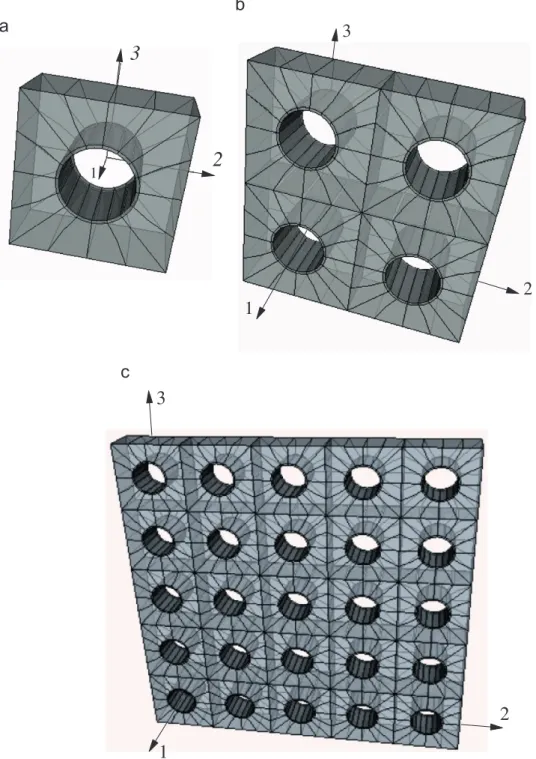
In this application, RVEs based on 11, 22, and 55 unit

cells are employed for modeling long-CNT-based composites (seeFig. 2). The length along the 1 direction (ﬁber direction) of the

specimen is the same as the CNT length (l1¼10 nm). The other

dimensions of each unit cell (along the 2 and 3 axes; seeFig. 2)

are taken as l2¼l3¼20 nm. Important model data are provided

inTable 1. InTable 2, the engineering parameters extracted from

the analysis of all the RVEs shown in Fig. 2 are compared

with results calculated by Liu and Chen [33]via ﬁnite-element

analysis, and estimated (when possible) by the rules of mixture

(see Refs.[33, 34]).

Table 1

Model data for the square-packed long-CNT RVEs.

Model nsuba _nelb _nnodesc _ndofd _{Sparsity (%)}

11 2 128 608 1824 29 22 8 512 2660 7980 81 55 50 1344 17,456 52,368 97

a_{n. of subregions} b_{n. of elements} c_{n. of nodes}

d_{n. of degrees of freedom}

Table 2

Engineering constants for the square-packed long-CNT RVEs.

Model E1/Em E2/Em,E3/Em n₁₂,n₁₃ n₂₃

11 1.3227 0.8302 0.2974 0.3595 22 1.3228 0.8319 0.2973 0.3600 55 1.3228 0.8319 0.2972 0.3580 Chen & Liu (3D FE) 1.3255 0.8492 0.3000 0.3799 Rule of mixturea _1.3255 _– _– _–

(6)

As seen fromTable 2, there is a very good agreement between the material parameters calculated with the present method and

estimated by reﬁned 3D FE models[33]or the rules of mixture

([22, 34]). Furthermore, no signiﬁcant change in the constant values is also observed as the number of unit cells per RVE increases.

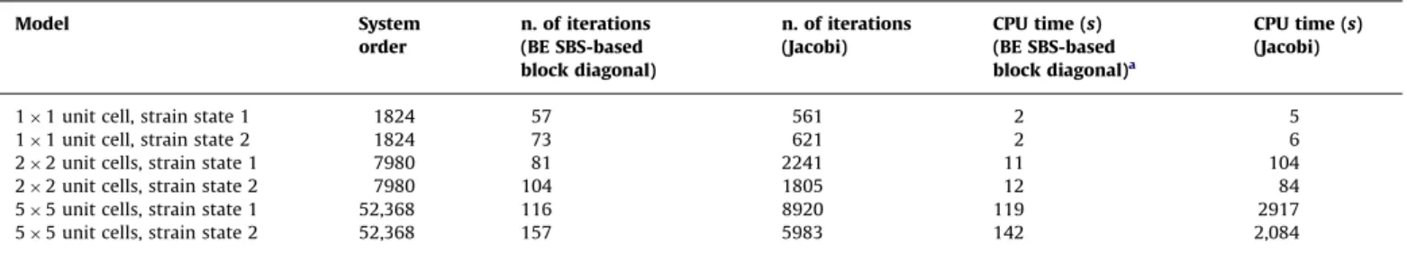
InTable 3, results showing the performance of the precondi-tioners are presented. As one sees, compared to the Jacobi preconditioner, a considerable acceleration of Bi-CG solver is observed when the BE SBS-based block-diagonal one is applied

(e.g. it makes the solver about 24 times faster for the 5

5-unit-cell RVE under strain state 1). Notice that, although the cost per iteration is higher using the BE SBS-based block-diagonal preconditioning, the corresponding number of iterations is considerably reduced. The decaying of the Euclidean residual

norm,:

d

_:

2, as a function of the iteration order for both contrasted

preconditioners is also shown in Fig. 3. This graph clearly

shows the superiority of the BE SBS-based block-diagonal preconditioning.

4.2. RVEs with hexagonal-packed long CNT fibers

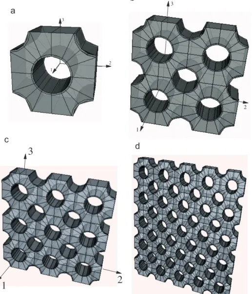
Here, 11, 22, 33, and 55 RVEs are analyzed (see

Fig. 4), each one built with unit cells having dimensionsl1¼10 nm

andl2¼l3¼20 nm. Model data and estimated material parameters

are given in Tables 4 and 5, respectively. For comparison

purposes, onlyE1, estimated by the rules of mixture, is considered

[34], and we verify that E1 values estimated by the rules of

mixture and calculated with the present method are about the same magnitude. Here we also note that increasing the number of unit cells per RVE does not signiﬁcantly change the estimated

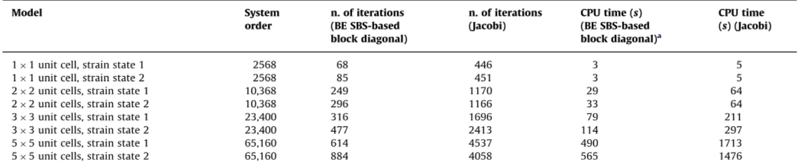
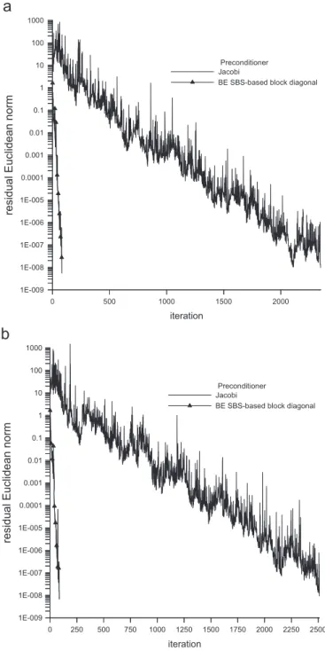
material constants. InTable 6the performance of both

precondi-tioners is presented, and in the graph inFig. 5the decaying of the

corresponding residual Euclidean norms during the Bi-CG itera-tions is given. Again, the performance of the BE SBS-based block-diagonal preconditioning has shown superior.

4.3. RVEs with squared-packed short CNT fibers

In this application, the RVEs are constituted of 11 and 22

short capsule-like CNTs smeared inside the matrix material along

square-packing patterns (Fig. 6,Table 7). A single-cell RVE has

outer dimensionsl1¼100 nm andl2¼l3¼20 nm, and the

geome-trical details of the CNT were furnished above. Compared to the

results obtained by Liu and Chen[33], and, when possible, by the

extended rule of mixture[22], the values estimated by applying

the BE SBS-based strategy show good agreement (Table 8). For

both RVEs, about the same material constant values are

estimated. In Table 9, performance data of the Jacobi and BE

SBS-based preconditioners are given. InFig. 7, the residual norm

decaying as a function of the iteration order is shown. Again, the

BE SBS-based preconditioning clearly increases the efﬁciency of

the Bi-CG solver, making it for the 22-unit-cell RVE under strain

state 1 about 10 times faster.

Table 3

Performance data for the square-packed long-CNT RVEs; tol¼1.0108_.

Model System

order

n. of iterations (BE SBS-based block diagonal)

n. of iterations (Jacobi)

CPU time (s₎

(BE SBS-based block diagonal)a

CPU time (s₎

(Jacobi)

11 unit cell, strain state 1 1824 57 561 2 5 11 unit cell, strain state 2 1824 73 621 2 6 22 unit cells, strain state 1 7980 81 2241 11 104 22 unit cells, strain state 2 7980 104 1805 12 84 55 unit cells, strain state 1 52,368 116 8920 119 2917 55 unit cells, strain state 2 52,368 157 5983 142 2,084

a_{Including the LU decomposition CPU time}

0 1000 2000 3000 4000 5000 6000 7000 8000 9000

iteration 1E-009

1E-008 1E-007 1E-006 1E-005 0.0001 0.001 0.01 0.1 1 10 100 1000

res

id

u

al

Euc

lid

e

a

n

orm

Preconditioner Jacobi

BE SBS-based block diagonal

0 1000 2000 3000 4000 5000

iteration

1E-009 1E-008 1E-007 1E-006 1E-005 0.0001 0.001 0.01 0.1 1 10 100 1000

residual Euclidean norm

BE SBS-based bock diagonal

(7)

5. Conclusions and prospects

Using a robust boundary-element subregion-by-subregion

(BE SBS) technique proposed in previous papers ([21, 35]), a

straightforward strategy for constructing block-diagonal precon-ditioners for BE systems of equations is presented. The perfor-mance of this preconditioning was veriﬁed by analyzing complex composite representative volume elements (RVEs).

Observing Tables 3, 6 and 9, and graphs inFigs. 3, 5 and 7,

we see that the BE-SBS-based block-diagonal preconditioning, compared to the Jacobi (diagonal) one, considerably accelerates the Bi-CG solver, making it in all cases analyzed several times faster. Moreover, it causes the decaying of the residual Euclidean norm as a function of the iteration order to be more regular (see Figs. 3, 5 and 7). In fact, the BE-SBS-based block-diagonal preconditioning states a transition (or connection) between direct and iterative solvers, in the sense that the less the number of interfaces, the closer to the global system matrix the preconditioning

1

2 3

1

2 3

Fig. 4.Hexagonal-packed long-CNT-based RVEs.

Table 4

Model data for the hexagonal-packed long-CNT RVEs.

11 6 138 856 2568 72 22 17 656 3456 10,368 86 33 34 1464 7800 23,400 93 55 86 4040 21,720 65,160 97

a_{n. of subregions} b_{n. of elements} c_{n. of functional nodes} d_{n. of degrees of freedom}

Table 5

Engineering constants for the hexagonal-packed long-CNT RVE.

Model E1/Em E2Em,E3/Em n12,n13 n23

11 1.8081 1.0889 0.2943 0.5107 22 1.8074 1.0839 0.2936 0.5107 33 1.8074 1.0916 0.2931 0.5185 55 1.8126 1.0813 0.2927 0.4997 Rule of mixturea _1.8131 _– _– _–

(8)

matrix,Q, is. For example, if no interface is present in the model, the

Qmatrix is identical to the system matrix (with one single or many

decoupled subregions), and convergence will be reached at one

Table 6

Performance data for the hexagonal-packed long-CNT RVEs; tol¼1.0108.

Model System

order

CPU time (s₎

CPU time (s) (Jacobi)

11 unit cell, strain state 1 2568 68 446 3 5 11 unit cell, strain state 2 2568 85 451 3 5 22 unit cells, strain state 1 10,368 249 1170 29 64 22 unit cells, strain state 2 10,368 296 1166 33 64 33 unit cells, strain state 1 23,400 316 1696 79 211 33 unit cells, strain state 2 23,400 477 2413 114 297 55 unit cells, strain state 1 65,160 614 4537 490 1713 55 unit cells, strain state 2 65,160 884 4058 565 1476

a_{Including the LU decomposition CPU time}

0 500 1000 1500 2000 2500 3000 3500 4000 4500

iteration

1E-009 1E-008 1E-007 1E-006 1E-005 0.0001 0.001 0.01 0.1 1 10 100 1000

res

idual Euclidean norm

0 500 1000 1500 2000 2500 3000 3500 4000

iteration

1E-009 1E-008 1E-007 1E-006 1E-005 0.0001 0.001 0.01 0.1 1 10 100

resid

ua

l Eu

c

lidean

norm

Fig. 5. Residual norm vs. iteration: 55-unit-cell, hexagonal-packed long CNT: (a) strain state 1 and (b) strain state 2.

Fig. 6.Square-packed short-CNT-based RVEs.

Table 7

Model data for the square-packed short-CNT RVEs.

11 2 352 1064 3192 27 22 8 1408 5156 15,468 78

a_{n. of subregions} b_{n. of elements} c_{n. of functional nodes} d_{n. of degrees of freedom}

Table 8

Engineering constants for the square-packed short-CNT RVEs.

Model E1/Em E2/Em,E3/Em n12,n13 n23

11 1.0378 0.9366 0.2963 0.3207 22 1.0379 0.9379 0.2976 0.3217 Chen & Liu (3D FE) 1.0391 0.9342 0.3009 0.3217 Rule of mixturea _1.0396 _– _– _–

(9)

single iteration. In addition, knowing that the global coupled system is highly sparse, we can well conclude that the preconditioner proposed will be certainly a good approximation of the global

system matrix, which is one of the requirements for finding good preconditioners. Generally speaking, the larger the size of the subsystems, the higher the cost for constructing the preconditioner, however, on the other hand, a better approximation for the global system is achieved, reducing then the number of iterations. Furthermore, being this preconditioner based on the BE-SBS algorithm, its parallelization is immediate. By the way, in a cost-benefit analysis, not only the acceleration of the iterative process but also the solver-convergence reliability and parallel-processing suitability should be considered as benefit.

Among others, we can ﬁnally afﬁrm that the BE-SBS strategy has the following general advantages: (1) it is a fundamental technique to model complex heterogeneous problems, (2) it is a spontaneous way

to parallelize BE codes[36], and (3) it is, as shown in this paper, an

easy way to construct efﬁcient block-diagonal preconditioners for the Krylov solver the BE-SBS algorithm itself embeds. Although reliable and fast convergence of iterative solvers is a still open question for general practical modeling in engineering, mainly in the case of BE formulations, where usually non-symmetric matrices are involved

[37], it seems that the BE-SBS-based block-diagonal preconditioner

proposed in this paper will be one more contribution towards making the reliable use of iterative solvers in engineering feasible. Of course, much more efﬁciency would have been attained if, compared to the Bi-CG solver, more efﬁcient Krylov solvers, as e.g. the

Bi-CGSTAB(l)[8]or the GPBi-CG[15], had been employed.

Acknowledgements

This research was sponsored by the Ofﬁce of Advanced Scientiﬁc Computing Research, U.S. Department of Energy under Contract DE-AC05-00OR22725 with UT-Battelle, LLC, the Brazilian Research Council (CNPq), and by the Research Foundation for the State of Minas Gerais (FAPEMIG), Brazil.

References

[1] van der Vorst HA. Iterative Krylov Methods for Large Linear Systems. Cambridge University Press; 2003.

[2] Saad Y. Iterative Methods for Sparse Linear Systems, Society for Industrial and Applied Mathematics. Philadelphia: SIAM; 2003.

[3] Lanczos C. Solution of systems of linear equations by minimized iteration. J Res Nat Bur Stand 1952;49:33–53.

[4] Fletcher R. Conjugate gradient methods for indeﬁnite systems, Lecture Notes in Mathematics 506. Berlin: Spriger-Verlag; 1976.

[5] Saad Y, Schultz MH. GMRES: a generalized minimum residual algorithm for solving nonsymmetric linear systems. SIAM J Sci Stat Comput 1986;7:856–69. [6] Sonneveld P. CGS, a fast Lanczos-type solver for nonsymetric linear systems.

SIAM J Sci Stat Comput 1989;10:36–52.

[7] van der Vorst HA. Bi-CGSTAB: a fast and smoothly converging variant of Bi-CG for the solution of nonsymmetric linear systems. SIAM J Sci Stat Comput 1992;13:631–44.

[8] Sleijpen GLG, Fokkema DR. BICGSTAB(L) for linear equations involving unsymmetric matrices with complex spectrum. Electron Trans Num Methods Anal 1993;1:11–32.

[9] Arau´jo FC, Mansur WJ. Iterative solvers for BEM systems of equations. In: Proceedings of the 11th International Conference on Boundary Element Methods, Cambridge, USA, 1989, vol. 1, pp. 263–274.

Table 9

Performance data for square-packed short-CNT RVEs; tol¼1.0108_.

Model System

order

CPU time (s₎

(Jacobi)

11 unit cell, strain state 1 3192 51 763 6 21 11 unit cell, strain state 2 3192 67 822 7 23 22 unit cells, strain state 1 15,468 83 2348 60 610 22 unit cells, strain state 2 15,468 87 2510 60 481

a_{Including the LU decomposition CPU time.}

0 500 1000 1500 2000

iteration

1E-009 1E-008 1E-007 1E-006 1E-005 0.0001 0.001 0.01 0.1 1 10 100 1000

residual E

u

clidean n

orm

0 250 500 750 1000 1250 1500 1750 2000 2250 2500

iteration

1E-009 1E-008 1E-007 1E-006 1E-005 0.0001 0.001 0.01 0.1 1 10 100 1000

re

sidua

l Euclidea

n

norm

(10)

[10] Arau´jo FC, Mansur WJ, Malaghini JEB. Biconjugate gradient acceleration for large BEM systems of equations In: Proceedings of the 12th International Conference on Boundary Element Methods, Sapporo, Japan, vol. 1, 1990, pp. 99–110.

[11] Kane JH, Keyes DE, Prasad KG. Iterative equation solution techniques in boundary element analysis. Int J Numer Methods Eng 1991;31:1511–36. [12] Mansur WJ, Arau´jo FC, Malaghini JEB. Solution of BEM systems of equations

via iterative techniques. Int J Numer Methods Eng 1992;33:1823–41. [13] Bettess JA. Economical solution techniques for boundary integral matrices.

Int J Numer Methods Eng 1983;19:1073–7.

[14] Mullen RL, Rencis JJ. Iterative methods for solving boundary element equations. Comput Struct 1987;25:713–23.

[15] Zhang S-L. A class of product-type Krylov-subspace methods for solving nonsymmetric linear systems. J Comp Appl Math 2002;149:297–305. [16] Vavasis SA. Preconditioning for boundary integral-equations. SIAM J Matrix

Anal Appl 1992;13:905–25.

[17] Chen K. Matrix Preconditioning Techniques and Applications. Cambridge, UK: Cambridge University Press; 2005.

[18] Davey K, Bounds S. A preconditioning strategy for the solution of linear boundary element systems using the GMRES method. Appl Numer Math 1997;23:443–56.

[19] Merkel M, Bulgakov V, Bialecki R, Kuhn G. Iterative solution of large-scale 3D-BEM industrial problems. Eng Anal Boundary Elem 1998;22:183–97. [20] Chen K. On a class of preconditioning methods for dense linear systems from

boundary elements. SIAM J Sci Comput 1998;20:684–98.

[21] Arau´jo FC, Silva KI, Telles JCF. Generic domain decomposition and iterative solvers for 3D BEM problems. Int J Numer Methods Eng 2006;68:448–72. [22] Arau´jo FC, Gray LJ. Evaluation of effective material parameters of

CNT-reinforced composites via 3D BEM. Comp Mod Eng Sci 2008;24(2):103–21. [23] Arau´jo FC, Dors C, Martins CJ, Mansur WJ. New developments on BE/BE

multi–zone algorithms based on Krylov solvers—applications to 3D

frequency-dependent problems. J Braz Soc Mech Sci Eng 2004;26(2):231–48.

[24] Li HB, Han GM, Mang HA. A new method for evaluating for evaluating singular integrals in stress analysis of solids by the direct boundary element method. Int J Numer Methods Eng 1985;21:2071–98.

[25] Telles JCF. A self-adaptive co-ordinate transformation for efﬁcient numerical evaluation of general boundary element integrals. Int J Numer Methods Eng 1987;24:959–73.

[26] Liu Y. Analysis of shell-like structures by the boundary element method based on 3-D elasticity: formulation and veriﬁcation. Int J Numer Methods Eng 1998;41:541–58.

[27] Chen XL, Liu YJ. An advanced 3D boundary element method for characteriza-tion of composite materials. Eng Anal Boundary Elem 2005;29:513–23. [28] Arau´jo FC, Gray LJ. Analysis of thin-walled structural elements via 3D

standard BEM with generic substructuring. Comput Mech 2008;41:633–45. [29] Hughes TJR, Levit I, Winget L. An element-by-element solution algorithm for

problems of structural and solid mechanics. Comput Methods Appl Mech Eng 1983;36(2):241–54.

[30] Farhat C, Roux F-X. An unconventional domain decomposition method for an efﬁcient parallel solution of large-scale ﬁnite element systems. SIAM J Sci Stat Comput 1992;13:379–96.

[31] Araujo FC, Belmonte GJ, Freitas MSR. Efﬁciency increment in 3D multizone boundary element algorithms by use of iterative solvers. J Chin Inst Eng 2000;23(3):269–74.

[32] Yu W, Wang Z, Hong X. Preconditioned multi-zone boundary element analysis for fast 3D electric simulation. Eng Anal Boundary Elem 2004;28(9):1035–44. [33] Chen XL, Liu YJ. Square representative volume elements for evaluating the effective material properties of carbon nanotube-based composites. Comput Mater Sci 2004;29:1–11.

[34] Hyer MW. Stress Analysis of Fiber-Reinforced Composite Materials. 1st ed.. Boston: McGraw-Hill; 1998.

[35] Arau´jo FC, Silva KI, Telles JCF. Application of a generic domain-decomposition strategy to solve shell-like problems through 3D BE models. Commun Numer Methods Eng 2007;23:771–85.

[36] Arau´jo FC, d’Azevedo EF, Gray LJ. Boundary-element parallel-computing algorithm for the microstructural analysis of general composites. Comput Struct 2010;88:773–84.