Boundary layer of the dissociated
gas flow over a porous wall under
the conditions of equilibrium
dissociation
Branko Obrovi´
c
∗, Dragiˇ
sa Nikodijevi´
c
†, Slobodan Savi´
c
‡Abstract
This paper studies the ideally dissociated air flow in the bound-ary layer when the contour of the body within the fluid is porous. By means of adequate transformations, the governing boundary layer equations of the problem are brought to a general form. The obtained equations are numerically solved in a three-parametric localized approximation. Based on the obtained solutions, very important conclusions about behaviour of certain boundary layer physical values and characteristics have been drawn.
Keywords: boundary layer, dissociated gas, equilibrium dis-sociation, porous contour, general similarity method, porosity parameter
∗Faculty of Mechanical Engineering University of Kragujevac Sestre Janji´c 6,
34000 Kragujevac, Serbia and Montenegro
†Faculty of Mechanical Engineering University of Niˇs, Aleksandra Medvedeva 14,
18000 Niˇs, Serbia and Montenegro
‡Faculty of Mechanical Engineering University of Kragujevac Sestre Janji´c 6,
34000 Kragujevac, Serbia and Montenegro, e-mail: [email protected]
Nomenclature
A, B boundary layer characteristics
a, b constants
Ci mass concentration of any i component
cp specific heat of gas dissociated at constant pressure D21=D12 =D coefficient of atomic component diffusion
Di diffusion coefficient of any i component
Fdp characteristic boundary layer function f1 =f first form parameter
fk set of form parameters
H boundary layer characteristic
h enthalpy
¯
h nondimensional enthalpy
he enthalpy at the outer edge of the boundary layer hi enthalpy of the mass unit of any i component
hw enthalpy at the wall of the body within the fluid
h1 enthalpy at the front stagnation point of the body within the fluid
Le Lewis number
l function
M discrete point
Pr Prandtl number
p pressure
Q nondimensional function
Ri gas constant of any i component
Smi Schmidt number (diffusion Prandtl number) of any
i component
s new longitudinal variable
u longitudinal projection of velocity in the boundary layer
ue velocity at the boundary layer outer edge
Vw conditional transversal velocity
v transversal projection of velocity in the boundary layer
vw velocity of injection (or ejection) of the fluid ˙
Wi mass formation rate of any i component
x, y longitudinal and transversal coordinate
Z∗∗
z new transversal variable ∆∗
conditional displacement thicknesses ∆∗∗
conditional momentum loss thickness
ζ nondimensional friction function
η nondimensional transversal coordinate
κ=f0 local compressibility parameter Λ1 = Λ first porosity parameter
Λk set of porosity parameters
λ thermal conductivity coefficient
µ dynamic viscosity
µ0 known values of dynamic viscosity of the dissociated gas
µw given distributions of dynamic viscosity at the wall
of the body within the fluid
ν0 kinematic viscosity at a concrete point of the boundary layer
ρ density of ideally dissociated gas
ρe dissociated gas density at the outer edge of the boundary layer
ρ0 known values of density of the dissociated gas
ρw given distributions of density at the wall of the body within the fluid
τw shear stress at the wall of the body within the fluid
Φ nondimensional stream function
ψ stream function
ψ∗
new stream function
1
Introduction
The main goal of this investigation, as with our earlier studies, is to apply the general similarity method to obtain the so-called generalized boundary layer equations of the considered problem, and to solve them. When the flow velocity of the gas (air) is high, as with supersonic flight of aircrafts through the Earth atmosphere, the temperature in the viscous boundary layer increases significantly. These high temperatures cause thermochemical reactions of dissociation and recombination. Due to the thermochemical processes in the boundary layer, the air becomes a multicomponent mixture of atomic and molecular components. There-fore, for the steady gas mixture flow followed with chemical reactions, the complete equation system of laminar planar boundary layer has the following form:
ρu ∂u ∂x +ρv
∂u ∂y =−
dp dx +
∂ ∂y
µ µ ∂u
∂y ¶
,
∂
∂x (ρu) + ∂
∂y (ρv) = 0,
ρu ∂Ci ∂x +ρv
∂Ci ∂y =
∂ ∂y
µ
ρ Di ∂Ci ∂y
¶
+ ˙Wi, (i= 1, 2, ..., q−1)
(1)
ρ u∂h ∂x +ρv
∂h
∂y = u dp dx +µ
µ ∂u ∂y
¶2 + ∂
∂y µ
µ
Pr
∂h ∂y
¶ +
∂ ∂y
" X
i
ρhiDi µ
1− Smi Pr
¶ ∂Ci
∂y #
,
p=ρRT ,¯ R¯ =X
i
CiRi, (X
i
Ci = 1 ).
The notations common in the boundary layer theory are used for cer-tain physical values in these equations [1, 2].
According to Lighthill, gas mixture flow can be replaced with a bi-nary mixture model consisting only of an atomic and a molecular com-ponent. Ideally dissociated gas is defined this way. Air at temperatures around 2 000 K and even up to around 8 000 K can be considered [1] an ideally dissociated gas. An ideally dissociated gas model can be ap-plied to the boundary layer flow. Then the mass concentration of the atomic component is defined as C1 = ρ1/ρ = ρA/ρ = CA = α; while the mass concentration of the molecular component is C2 = ρ2/ρ =
ρM/ρ =CM = 1−α , where the subscripts A and M stand for atomic, i.e., molecular component of the ideally dissociated gas.
When dissociation and recombination velocities are high enough, thermochemical equilibrium is established in the boundary layer. In that case the concentration C1 = α is directly related to the absolute temperature i.e. enthalpy.
If it is assumed that the thermochemical equilibrium is established in the whole boundary layer area, then [3, 4], the boundary layer equations (15) can be written in the following form:
∂
∂x (ρu) + ∂
∂y (ρv) = 0,
ρ u∂u ∂x +ρv
∂u
∂y = ρeue due
dx + ∂ ∂y
µ µ∂u
∂y ¶
, (2)
ρ u∂h ∂x +ρv
∂h
∂y = −u ρeue due
dx +µ µ
∂u ∂y
¶2
+ ∂
∂y ·
µ
Pr (1 +l)
∂h ∂y ¸
.
Compressible fluid flow problems have been investigated by scientists all around the world as well as in Serbia, especially by Saljnikov [10] to-gether with the members of the so-called Belgrade School of Boundary Layer. To our knowledge, the most important results obtained by in-vestigation of the dissociated gas flow were presented by Dorrance in [1]. Members of the School led by Loitsianskii [8] also obtained some important results in the field of dissociated gas flow in the boundary layer.
This paper presents the results of investigation of the ideally dissoci-ated gas (air) flow under conditions of equilibrium dissociation where the wall of the body within the fluid isporous. These results were obtained by application of the general similarity method firstly suggested by Loit-sianskii, and later improved by Saljnikov, but mostly for its application to incompressible fluid flow in the boundary layer.
The corresponding boundary conditions of the considered flow prob-lem are:
u= 0, v =vw(x), h=hw for y= 0,
u→ue(x), h→he(x) for y→ ∞. (3)
In the governing equations of the system (2), as well as in the bound-ary conditions (3), the usual notations are used: u(x, y) - longitudinal projection of velocity in the boundary layer, v(x, y) - transversal pro-jection, ρ - density of ideally dissociated gas (mixture), µ - dynamic viscosity, h- enthalpy, Pr - Prandtl number, and x,y- longitudinal and transversal coordinate. The Function l = l(p, h) for the equilibrium bicomponential mixture is determined by the expression [3],
l= (Le−1) (hA−hM) µ
∂CA ∂h
¶
p
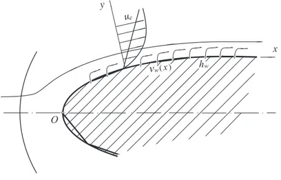
, (4)
body within the fluid (Fig.1). Here, vw >0 at injection, andvw <0 at
ejection of the gas.
O
w w
v ue
. . . .
y
h
x
Figure 1: Flow in the boundary layer
The nondimensional transfer coefficient, Prandtl and Lewis number are defined with the known expressions:
P r= µ cp
λ , Le= ρ cpD
λ (5)
where λ is thermal conductivity coefficient, cp - specific heat of gas dissociated at constant pressure and D21 = D12 = D - coefficient of atomic component diffusion. These numbers can be regarded as constant values [1, 3]. In our further studies Prandtl number is considered to be Pr = 0.712.
2
Transformation of boundary layer
equa-tions
s= 1
ρ0µ0
x Z
0
ρwµw∂x=s(x); z = 1
ρ0
y Z
0
ρ∂y =z(x, y), (6)
The stream function ψ(s, z) is also introduced in accordance with the relations:
u= ∂ψ
∂z , v˜= ρ0µ0
ρwµw µ
u∂z ∂x +v
ρ ρ0
¶
=−∂ψ
∂s, (7)
which result from the continuity equation.
In the expressions (6) and (7)ρ0 andµ0 =ρ0ν0 stand for the known values of density and dynamic viscosity of the dissociated gas (air). Here,
ρw and µw denote the given distributions of these values at the wall of the body within the fluid, and ν0 stands for kinematical viscosity at a concrete point of the boundary layer.
From the first two equations of the system (2), by a usual procedure – by integration transversally to the boundary layer and by transformation of the variables, the momentum equation of the considered problem is obtained. In its all three forms, the corresponding momentum equation is: dZ∗∗ ds = Fdp ue , df ds = u′ e ueFdp+
u′′ e u′ e f, 1 ∆∗∗
d∆∗∗
ds = u′
e ue
Fdp
2f . (8)
While obtaining the momentum equation, the following values are introduced: parameter of the form f, value Z∗∗
, conditional displace-ment thicknesses ∆∗
(s) and ∆∗∗
(s) conditional momentum loss thick-ness, nondimensional friction function ζ(s), porosity parameter Λ(s), characteristic function Fdp and nondimensional valueH. With this flow problem we have:
f(s) = u ′
e∆
∗∗2
ν0
=u′
eZ
∗∗
=f1, Z ∗∗ = ∆ ∗∗2 ν0 , ∆∗ (s) =
∆∗∗ (s) =
∞ Z 0 u ue µ
1 − u
ue ¶
dz ,
ς(s) = ·
∂(u/ue)
∂(z/∆∗∗) ¸
z=0
, H = ∆ ∗
∆∗∗, (9)
Fdp = 2[ς −(2 +H)f]−2Λ,
Λ(s) =−vwµ0
µw
∆∗∗
ν0
=−Vw∆ ∗∗
ν0
= Λ1,
Vw = µ0
µwvw;
where the value Vw(s) can be named conditional transversal velocity at the inner edge of the boundary layer. (In these expressions and further on ’ stands for a derivative with respect to the variable s).
Applying the transformations of the variables (6) and the stream function (7), the governing system (2), (3) of the considered dissociated gas flow problem comes down to the following equation system:
∂ψ ∂z
∂2ψ
∂s∂z − ∂ψ
∂s ∂2ψ
∂z2 =
ρe ρueu
′
e+ν0
∂ ∂z µ Q ∂ 2ψ ∂z2 ¶ , ∂ψ ∂z ∂h ∂s − ∂ψ ∂s ∂h
∂z = − ρe
ρueu
′
e ∂ψ
∂z +ν0Q µ
∂2ψ
∂z2 ¶2 + (10) ν0 ∂ ∂z · Q
P r (1 +l) ∂h ∂z ¸
;
∂ψ ∂z = 0,
∂ψ ∂s =−
µ0
µwvw =−Vw, h =hw f or z = 0,
∂ψ
The nondimensional function Q is determined as:
Q = ρ µ
ρwµw ; Q= 1 f or z = 0,
(11)
Q → ρeµe
ρwµw =Q(s) f or z → ∞.
As seen from the expression (8), the momentum equation is by its form the same as the momentum equation of incompressible fluid [8]. And the dynamic equation of the system (10) has a similar form to the corresponding equation of incompressible fluid.
However, it is noticed that the (underlined) boundary layer condition for a partial derivative is∂ψ/∂s6= 0.With the application of the general similarity method, it is important that this boundary layer condition should equal zero. Therefore, as with incompressible fluid, [8] the stream function ψ(s, z) is divided into two parts. If the notation ψ(s, 0) =
ψw(s) is introduced for the stream function for the flow along the wall of the body (z = 0), then the stream function for this flow problem can be written in the form of the relation
ψ(s, z) = ψw(s) +ψ∗
(s, z), ψ∗
(s, 0) = 0. (12)
where ψ∗
(s, z) is a new stream function.
When we apply the relation (12), the equation system (10) trans-forms into the system:
∂ψ∗
∂z
∂2ψ∗
∂s∂z − ∂ψ∗
∂s
∂2ψ∗
∂z2 −
dψw ds
∂2ψ∗
∂z2 =
ρe ρueu
′
e+ν0
∂ ∂z
µ Q ∂
2ψ∗
∂z2 ¶
,
∂ψ∗
∂z ∂h ∂s −
∂ψ∗
∂s ∂h ∂z −
dψw ds
∂h
∂z = − ρe
ρueu
′
e ∂ψ∗
∂z +ν0Q µ
∂2ψ∗
∂z2 ¶2
+
(13)
ν0
∂ ∂z
· Q
P r(1 +l) ∂h ∂z ¸
ψ∗
(s, z) = 0, ∂ψ
∗
∂z = 0, h=hw f or z= 0,
∂ψ∗
∂z →ue(s), h→he(s) f or z → ∞.
Each of the equations of the system (13) contains one (underlined) term on the left, where dψw/ds appears. It is noticed that
dψw(s)
ds = µ
∂ψ ∂s
¶
z=0
=−µ0
µwvw =− Vw. (14)
In the case of a nonporous wall of the body within the fluid (for which vw = 0), in the equations of the system (13) the underlined terms equal zero, therefore the obtained equation system is exactly the same as the corresponding system [3]. The characteristic function Fdp comes
down to the corresponding function F.
3
Generalized boundary layer equations of
the considered flow problem
In accordance with the ideas followed with the application of the general similarity method to different flow problems for both compressible and incompressible fluid [6, 7], in these studies we introduced new variables and a new stream function Φ(s, η). However, after comprehensive and rather complicated numerical transformations, it has been determined that, here also, new transformations should be introduced in the form of the following expressions:
s = s; η(s, z) = u
b/2
e (s) K(s) z ,
K(s) =
aν0 s Z
0
ub−1
e ds
1/2
ψ∗
(s, z) =u1−b/2
e K(s) · Φ (η , κ , f1, f2, f3, ... , Λ1,Λ2,Λ3, ...), (15)
h(s, z) = h1·¯h(η , κ , f1, f2, f3, ... , Λ1,Λ2,Λ3, ...),
µ he+u
2
e
2 =h1 =const. ¶
In defined so-called similarity transformations, the following nota-tions are used: η(s, z) - newly introduced transversal variable, Φ - new stream function, ¯h- nondimensional enthalpy, and h1 - enthalpy at the front stagnation point of the body within the fluid.
Here also, based on the newly introduced transversal variableη(s, z), important values and characteristics of the boundary layer (9) can be written in the form of suitable relations:
∆∗∗
= K(s)
ube/2
B(s), ∆
∗
∆∗∗ =H =
A(s)
B(s) ,
f B2 =
a u′
e ub
e s Z
0
ub−1
e ds ,
ζ =B µ
∂2Φ
∂η2 ¶
η=0
, τw = µ
µ∂u ∂y
¶
y=0
= ρwµw
ρ0
ue
∆∗∗ ζ , (16)
A(s) = ∞ Z
0 µ
ρe ρ −
∂Φ
∂η ¶
dη , B(s) = ∞ Z
0
∂Φ
∂η µ
1− ∂Φ
∂η ¶
dη ;
where the values A and B are assumed to be continual functions of the longitudinal variable s. The local parameter of dissociated gas com-pressibility [4] κ = f0, the set of parameters of the form fk(s) of
Loit-sianskii’s type [8], as well as the set of porous wall parameters [9] Λk(s)
κ=f0(s) = u 2 e
2h1 , fk(s) = u k−1
e u
(k)
e Z∗∗k,
Λk(s) =−uke−1 µ
Vw √ν 0
¶(k−1)
Z∗∗k−1/2
k = 1, 2, 3...).
(17)
For k = 1 we obtain f1(s) = u′e Z
∗∗
- a form parameter already known in the boundary layer theory, while the porosity parameter Λ1 = −(Vw∆∗∗
/ν0) is the same as the earlier defined parameter (9). Parame-ters of the sets (17) satisfy recurrent simple differential equations of the form: ue u′ e f1 dκ
ds = 2κ f1 ≡θ0, ue
u′
e f1
dfk
ds = [ (k−1) f1+k Fdp] fk+fk+1 ≡θk, (18)
ue u′
e f1
dΛk
ds ={(k−1)f1+ [ (2k−1)/2 ] Fdp} Λk+ Λk+1 ≡χk.
Applying the similarity transformations (15), (17) to the equation system (13) the generalized boundary layer equation system has been obtained. The outer velocity ue(s) appears explicitly in neither of the equations of the obtained system.
The obtained generalized equation system, together with the trans-formed boundary conditions, is:
∂ ∂η µ Q ∂ 2Φ ∂η2 ¶ +aB
2+ (2−b)f 1
2B2 Φ
∂2Φ
∂η2 +
f1 B2 " ρe ρ − µ ∂Φ ∂η ¶2#
+
Λ1
B ∂2Φ
∂η2 = 1 B2 " ∞ X k=0 θk µ ∂Φ ∂η
∂2Φ
∂η ∂fk − ∂Φ
∂fk ∂2Φ
∂η2 ¶ + ∞ X k=1 χk µ ∂Φ ∂η
∂2Φ
∂η ∂Λk − ∂Φ
∂Λk ∂2Φ
∂η2 ¶
∂ ∂η
· Q
P r(1 +l) ∂¯h ∂η ¸
+ aB
2+ (2−b)f 1
2B2 Φ
∂¯h ∂η −
2κ f1
B2
ρe ρ
∂Φ
∂η + 2κQ µ
∂2Φ
∂η2 ¶2
+ Λ1
B ∂¯h ∂η =
1
B2 · ∞
P k=0
θk µ
∂Φ
∂η ∂¯h ∂fk −
∂Φ
∂fk ∂¯h ∂η
¶ +
∞ P k=1
χk µ
∂Φ
∂η ∂¯h ∂Λk −
∂Φ
∂Λk ∂¯h ∂η
¶# ;
(19)
Φ = 0, ∂Φ
∂η = 0, ¯h= ¯hw =const. f or η= 0,
∂Φ
∂η →1 , ¯h→¯he(s) = 1−κ f or η→ ∞ .
Both equations of the system (19), on the left hand-side, contain one term that depends on the porosity parameter Λ1. On the right hand-side, each of the equations contains a sum of terms that are multiplied with the function χk. In the case of a non-porous wall (vw = 0, Vw = 0) all the porosity parameters equal zero, therefore these terms also equal zero. In that case, the obtained equations take the form of the corresponding equations [3] for the case of a flow along a non-porous wall.
κ can be performed in relation to the nondimensional total enthalpy
g = (h+u2/2)/h
1,i.e., it is justified to assume that∂g/∂κ≈0. There-fore in the three-parametric (f0 = κ 6= 0, f1 = f 6= 0, Λ1 = Λ 6= 0, f2 = f3 = ... = 0,Λ2 = Λ3 = ... = 0) twice localized approxima-tion (∂/∂κ= 0, ∂/∂Λ1 =0), the corresponding boundary layer equation system of the considered flow problem has the following form:
∂ ∂η µ Q∂ 2Φ ∂η2 ¶ +aB
2+ (2−b)f
2B2 Φ
∂2Φ
∂η2 +
f B2 " ρe ρ − µ ∂Φ ∂η ¶2#
+
Λ
B ∂2Φ
∂η2 =
Fdpf B2
µ ∂Φ
∂η
∂2Φ
∂η ∂f − ∂Φ
∂f ∂2Φ
∂η2 ¶ , ∂ ∂η · Q
P r (1 +l) ∂¯h ∂η ¸
+aB
2+ (2−b)f
2B2 Φ
∂h¯ ∂η −
2κ f B2 ∂Φ ∂η " ρe ρ − µ ∂Φ ∂η ¶2#
+ 2κ Q µ
∂2Φ
∂η2 ¶2
+
+Λ
B ∂¯h ∂η = Fdpf B2 µ ∂Φ ∂η ∂¯h ∂f −
∂Φ
∂f ∂h¯ ∂η
¶
; (20)
Φ = 0, ∂Φ
∂η = 0, ¯h= ¯hw =const. f or η= 0 ,
∂Φ
∂η →1, h¯ →he¯ (s) = 1−κ f or η→ ∞ .
4
Numerical solution of the transformed
equation system. Obtained results
In papers [3, 4] it is stated that for dissociated airLe≈1.It follows that the function l (which is a part of the energy equation) is defined with the expression (4) and that it equals zero. Furthermore, in the papers written by the same author, based on the tables of the thermodynamic functions for air, it is proven that the following very correct approximate formula can be applied for the wide range of pressure changes:
Q(¯h) = µ¯ hw ¯ h ¶1/3 , (21)
and it is used in this paper.
For the density ratio in this paper, we used the approximationρe/ρ≈
¯
h/(1−κ) obtained from the corresponding rather complicated formula stated in [3].
Besides the previous relations for certain physical values, for numer-ical integration of the system (20), it is necessary to decrease the order of the dynamic equation. Introducing the transformation
u ue =
∂Φ
∂η =ϕ=ϕ (η , κ , f , Λ) , (22)
the order of the dynamic equation is decreased; therefore the correspond-ing equation system of the considered dissociated air flow problem takes the following form:
∂ ∂η µ Q∂ϕ ∂η ¶ +aB
2+ (2−b)f
2B2 Φ
∂ϕ ∂η+ f B2 µ ¯ h
1−κ − ϕ
2 ¶ + Λ B ∂ϕ ∂η = = Fdpf B2 µ ϕ ∂ϕ ∂f − ∂Φ ∂f ∂ϕ ∂η ¶ , ∂ ∂η µ Q P r
∂¯h ∂η
¶ + aB
2+ (2−b) f
2B2 Φ
∂¯h ∂η−
2κf B2 ϕ
µ ¯
h
1−κ−ϕ
2 ¶
= Fdpf
B2 µ
ϕ∂¯h ∂f −
∂Φ
∂f ∂¯h ∂η
¶
; (23)
Φ = 0, ϕ= 0, ¯h= ¯hw =const. f or η= 0 ,
ϕ →1 , h¯→he¯ (s) = 1−κ f or η→ ∞ .
Numerical solution of the obtained system of nonlinear and conjugated differential partial equations (23) is performed by the finite differences method, i.e., so-called ”passage method”. According to the usual scheme of the finite differences, the equation system (23) is firstly transformed into an equivalent system of algebraic equations, which is solved by it-erative procedure, taking into consideration the order of calculation of certain functions and linearization. The values of the functionsϕ, Φ, ¯h
are calculated at discrete points M of the half planar integration grid, i.e., at discrete points of each calculating layer (K+1). For each calcu-lating layer with this, as well as other complicated boundary layer fluid flow problem [6, 7], the number of discrete points N = 401 has been determined.
For the concrete solution of the equation system (23), i.e., for the solution of the corresponding algebraic system, the necessary program in FORTRAN has been written. It is based on the program used in [10]. All the necessary calculations have been made for the concrete values of
a and b , and they are: a = 0.4408 ; b = 5.7140 ; which, according to [10], represent the optimal values. For the Prandtl number, as already stated, for the case of dissociated air flow Pr = 0.712. While calculating the characteristic functions B and Fdp , at a zero iteration, the values
B0
K+1 = 0.469 and Fdp,K0 +1 = 0.4411,were accepted, as already done in the paper [10 ].
Table 1: One of the solutions of the dissociated gas boundary layer equations
f = 0.0000000D+ 00 Λ = 0.02 ∆f = 0.1000000D−02
A=−0.1758993 B = 0.5415912 B2 = 0.2933210
f /B2 = 0.0000000 H =−0.3247825 ∂2Φ/∂η2 = 0.6111155
Fdp = 0.6219525 κ= 0.04 ς = 0.3309762
M η u/ue Φ h Q
M η u/ue Φ h Q
177 8.8000001 1.0000000 7.1928120 0.9600000 0.2511062 185 9.2000001 1.0000000 7.5928120 0.9600000 0.2511062 193 9.6000001 1.0000000 7.9928120 0.9600000 0.2511062 201 10.0000001 1.0000000 8.3928120 0.9600000 0.2511062 209 10.4000002 1.0000000 8.7928120 0.9600000 0.2511062 217 10.8000002 1.0000000 9.1928120 0.9600000 0.2511062 225 11.2000002 1.0000000 9.5928120 0.9600000 0.2511062 233 11.6000002 1.0000000 9.9928120 0.9600000 0.2511062 241 12.0000002 1.0000000 10.3928120 0.9600000 0.2511062 249 12.4000002 1.0000000 10.7928120 0.9600000 0.2511062 257 12.8000002 1.0000000 11.1928120 0.9600000 0.2511062 265 13.2000002 1.0000000 11.5928120 0.9600000 0.2511062 273 13.6000002 1.0000000 11.9928120 0.9600000 0.2511062 281 14.0000002 1.0000000 12.3928121 0.9600000 0.2511062 289 14.4000002 1.0000000 12.7928121 0.9600000 0.2511062 297 14.8000002 1.0000000 13.1928121 0.9600000 0.2511062 305 15.2000002 1.0000000 13.5928121 0.9600000 0.2511062 313 15.6000002 1.0000000 13.9928121 0.9600000 0.2511062 321 16.0000002 1.0000000 14.3928121 0.9600000 0.2511062 329 16.4000002 1.0000000 14.7928121 0.9600000 0.2511062 337 16.8000003 1.0000000 15.1928121 0.9600000 0.2511062 345 17.2000003 1.0000000 15.5928121 0.9600000 0.2511062 353 17.6000003 1.0000000 15.9928121 0.9600000 0.2511062 361 18.0000003 1.0000000 16.3928121 0.9600000 0.2511062 369 18.4000003 1.0000000 16.7928121 0.9600000 0.2511062 377 18.8000003 1.0000000 17.1928121 0.9600000 0.2511062 385 19.2000003 1.0000000 17.5928121 0.9600000 0.2511062 393 19.6000003 1.0000000 17.9928121 0.9600000 0.2511062 401 20.0000003 1.0000000 18.3928121 0.9600000 0.2511062
This solution describes the dissociated gas flow in the laminar bound-ary layer along a flat plane (ue = u∞ = const, f = u
′
eZ
∗∗
= 0, κ =
different values of the porosity parameter. The diagram ¯h(η) is espe-cially shown for different values of the compressibility parameter at the cross-section of the boundary layer defined with f = 0.0 (Fig.8).
5
Discussion of the obtained results and
conclusions
Based on the given (and other) diagrams the general conclusion that the profiles of the obtained solutions of the boundary layer equations, concerning their behaviour, are the same as with other similar flow prob-lems.
For the considered flow case, the following conclusions can be defined:
• Nondimensional velocity u/ue at different cross-sections of the
boundary layer (differentf) converges very fast towards one (Fig.2).
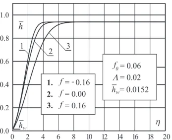
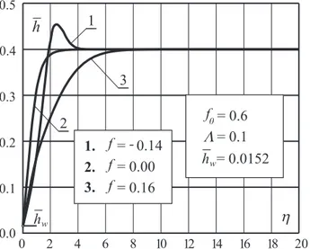
• A significant influence of the compressibility parameter κ on the distribution of the nondimensional enthalpy with respect to the boundary layer cross-section is noticed. The compressibility pa-rameter changes even the general character of behaviour of the enthalpy distribution in the boundary layer. For lower values of
κ ,the enthalpy ¯hreaches the maximum value that equals 1−κ ,at the outer edge of the boundary layer (Fig.3). However, for higher values of κ , the enthalpy ¯h has a maximum ¯hmax >1−κ within the boundary layer itself (Fig.8).
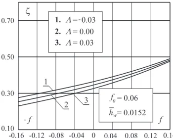
• The diagram (Fig.7) clearly shows that the porosity parameter Λ has an influence on the nondimensional friction function ζ, and therefore on the boundary layer separation point. We can also no-tice a great influence of this parameter on other important bound-ary layer characteristics: the valueB (Fig.5) and the function Fdp
(Fig.6).
Generally, there are some difficulties in application of the general similarity method to the problem of ideally dissociated air flow in the boundary layer around the porous contour. They are mainly of mathematic nature. The difficulties concerning physical, i.e., thermochemical problems of the gas flow itself are almost insolu-ble. This method, however, gives important quality results that enable us to study the behaviour of distributions of physical and characteristic values for different boundary layer cross-sections and different forms of the outer velocity functions.
• In order to obtain the more correct (quantity) results, it is neces-sary to integrate the system (19) in a three-parametric approxima-tion but without localizaapproxima-tion with respect to the parameter Λ, and especially without localization with respect to the compressibility parameter κ = f0. According to some earlier studies [5], it can be expected that this flow problem would show that the change of the compressibility parameter has a great influence on the change of the enthalpy in the boundary layer.
= 0.0152
w
f0= 0.4
f= 0.18
1.
2.
3.
f= 0.00 f=-0.18 1
2 3
0 2 4 6 8 10 12 14 16 18 20
0.0 0.2 0.4 0.6 0.8 1.0
u ue
h
h
= 0.1
L
Figure 2: Diagram of nondimensional velocity u/ue
1
2 3
0 2 4 6 8 10 12 14 16 18 20 0.2
0.4
0.0 0.6 0.8 1.0
f= 0.00 2.
f= 0.16 3.
f= 0.16 1.
-= 0.50
0
= 0.0152
w
= 0.06 f
= 0.02 L
h h
h
w
h
.
1
2
3
0 2 4 6 8 10 12 14 16 18 20 0.1
0.2
0.0 0.3 0.4 0.5
f= 0.00 2.
f= 0.16 3.
f= 0.14 1.
-= 0.50
0
= 0.0152 = 0.6 f
= 0.1 L
h
w
h
w
h h
.
Figure 4: Diagram of nondimensional enthalpy (κ =f0 = 0.6)
0= 0.04
f
= 0.0152
w
h
2
3 1
0.20 0.30
0.10 0.40 0.50 0.60 0.70 0.80
f f
-B
-0.16 -0.12 -0.08 -0.04 0 0.04 0.08 0.12 0.16
2.
3.
= 0.02
= 0.04
= 0.06
1. L
L L
0= 0.06 f
= 0.0152
w h
L L L
2.
3.
=- 0.03
= 0.00
= 0.03 1.
3 2
1
0.20 0.40 0.60 0.80 1.00 1.20 1.40
f f
-F
-0.16 -0.12 -0.08 -0.04 0 0.04 0.08 0.12 0.16
dp
Figure 6: Diagram of characteristic function Fdp(Λ)
0= 0.06
f
= 0.0152 w
h
L L L
2.
3.
= 0.03
= 0.00
= 0.03
1.
2 3
1
0.30
0.10 0.50 0.70
f f
--0.16 -0.12 -0.08 -0.04 0 0.04 0.08 0.12 0.16 z
3
4 2
1
0 2 4 6 8 10 12 14 16 18 20 0.2
0.4
0.0 0.6 0.8 1.0
2.
3.
4. 1.
0= 0.0
f
0= 0.5
f
0= 0.7
f
0= 0.9
f
h
= 0.0152 = 0.0 f
= 0.1
L
w
h
h
w
h
.
Figure 8: Diagram of nondimensional enthalpy in the cross-section of the boundary layer when f = 0.0 for different values of parameter κ=f0
References
[1] W. H. Dorrance, Viscous hypersonic flow, Theory of reacting and hy-personic boundary layers (in Russian), Mir, Moscow, 1966.
[2] John D. Jr. Anderson, Hypersonic and high temperature gas dynamics, McGraw-Hill Book Company, New York, St. Louis, San Francisco, 1989.
[3] N. V. Krivtsova, Parameter method of solving of the laminar boundary layer equations with axial pressure gradient in the conditions of balance dissociation of the gas (in Russian), Engineering-Physical Journal, X, (1966), 143-153.
[4] N. V. Krivtsova, Laminar boundary layer with the equilibrium dissoci-ated gas (in Russian), Gidrogazodinamika, Trudi LPI, No. 265, (1966), 35-45.
[5] B. Obrovic, Boundary layer of dissociated gas (in Serbian), Monograph, University of Kragujevac, Faculty of Mechanical Engineering, Kraguje-vac, 1994.
Series ”Mechanics, Automatic Control and Robotics”, Vol. 3, No. 15, (2003), 989-1000.
[7] B. Obrovic and S. Savic, Ionized gas boundary layer on a porous wall of the body within the electroconductive fluid, Theoret. Appl. Mech., Vol. 31, No. 1, (2004), 47-71.
[8] L. G. Loitsianskii, Liquid and gas mechanics (in Russian), Nauka, Moscow, 1973, 1978.
[9] B. Obrovic and S. Savic, About porosity parameters with the application of the general similarity method to the case of a dissociated gas flow in the boundary layer, Kragujevac J. Math. 24, (2002), 207-214.
[10] V. Saljnikov and U. Dallmann, Verallgemeinerte Ahnlichkeitslosungen fur dreidimensionale, laminare, stationare, kompressible Grenzschicht-stromungen an schiebenden profilierten Zylindern. Institut fur Theo-retische Stromungsmechanik, DLR-FB 89-34, Gottingen, 1989.
Submitted on July 2005.
Graniˇ
cni sloj strujanja disociranog gasa preko
poroznog zida u uslovima ravnoteˇ
zne disocijacije
UDK 532.526