Theoretical framework for estimating snow distribution through point measurements

(1)

TCD

9, 1–44, 2015

Theoretical framework for estimating snow distribution through point measurements

E. Trujillo and M. Lehning

Title Page

Abstract Introduction

Conclusions References

Tables Figures

◭ ◮

Back Close

Full Screen / Esc

Printer-friendly Version

Interactive Discussion

Discussion

P

a

per

|

Discussion

P

a

per

|

Discussion

P

a

per

|

Discussion

P

a

per

|

The Cryosphere Discuss., 9, 1–44, 2015 www.the-cryosphere-discuss.net/9/1/2015/ doi:10.5194/tcd-9-1-2015

This discussion paper is/has been under review for the journal The Cryosphere (TC). Please refer to the corresponding final paper in TC if available.

Theoretical framework for estimating

snow distribution through point

measurements

E. Trujillo1and M. Lehning1,2

1

Laboratory of Cryospheric Sciences, School of Architecture, Civil and Environmental Engineering, École Polytechnique Fédérale de Lausanne, Lausanne, Switzerland

2

WSL Institute for Snow and Avalanche Research SLF, Davos, Switzerland

Received: 28 November 2014 – Accepted: 1 December 2014 – Published: 5 January 2015 Correspondence to: E. Trujillo (ernesto.trujillo@epfl.ch)

(2)

TCD

9, 1–44, 2015

Title Page

Tables Figures

◭ ◮

Back Close

Full Screen / Esc

Discussion

P

a

per

|

Discussion

P

a

per

|

Discussion

P

a

per

|

Discussion

P

a

per

|

Abstract

In recent years, marked improvements in our knowledge of the statistical properties of the spatial distribution of snow properties have been achieved thanks to improvements in measuring technologies (e.g. LIDAR, TLS, and GPR). Despite of this, objective and quantitative frameworks for the evaluation of errors and extrapolations in snow

mea-5

surements have been lacking. Here, we present a theoretical framework for quantita-tive evaluations of the uncertainty of point measurements of snow depth when used to represent the average depth over a profile section or an area. The error is defined as the expected value of the squared difference between the real mean of the profile/field and the sample mean from a limited number of measurements. The model is tested for

10

one and two dimensional survey designs that range from a single measurement to an increasing number of regularly-spaced measurements. Using high-resolution (∼1 m) LIDAR snow depths at two locations in Colorado, we show that the sample errors follow the theoretical behavior. Furthermore, we show how the determination of the spatial lo-cation of the measurements can be reduced to an optimization problem for the case of

15

the predefined number of measurements, or to the designation of an acceptable uncer-tainty level to determine the total number of regularly-spaced measurements required to achieve such error. On this basis, a series of figures are presented that can be used to aid in the determination of the survey design under the conditions described, and under the assumption of prior knowledge of the spatial covariance/correlation

prop-20

(3)

TCD

9, 1–44, 2015

Title Page

Tables Figures

◭ ◮

Back Close

Full Screen / Esc

Discussion

P

a

per

|

Discussion

P

a

per

|

Discussion

P

a

per

|

Discussion

P

a

per

|

1 Introduction

The assessment of uncertainties of snow measurements remains a challenging prob-lem in snow sciences. Snow cover properties are highly heterogeneous over space and time and the representativeness of measurements of snow stage variables (e.g. snow depth, snow density, and snow water equivalent – SWE) is often overlooked due to

5

difficulties associated with the assessment of such uncertainties. This has been, at least in part, due to the limited knowledge of the characteristics of the spatial statistical properties of variables such as snow depth and SWE, particularly at the small-scales (sub-meter to tens of meters). However, a turning point has been reached in recent years thanks to improvements in remote sensing of snow (e.g. light detection and

rang-10

ing (LiDAR) and Radar technologies), which have allowed significant progress in the quantitative understanding of the small-scale heterogeneity of snow covers in different environments, with resolutions and areas of coverage previously unresolved with the standard methods of measurement (e.g. Trujillo et al., 2007, 2009; Mott et al., 2011).

Point or local measurements of snow properties will continue to be necessary for

pur-15

poses that range from inexpensive evaluation of the amount of snow over a particular area, to validation of models and remote sensing measurements. Such measurements have a footprint representative of a very small area surrounding the measurement lo-cation (i.e. support, following the nomenclature proposed by Blöschl, 1999), and the integration of several measurements is necessary for a better representation of the

20

snow variable in question over a given area. Because of this, tools for quantitative evaluations of the representativeness and uncertainty of measurements need to be in-troduced, and the uncertainty of such measurements should be more widely discussed in the field of snow sciences.

Currently, efforts to assess the reliability and uncertainty of snow measurements

25

(4)

Kro-TCD

9, 1–44, 2015

Title Page

Tables Figures

◭ ◮

Back Close

Full Screen / Esc

Discussion

P

a

per

|

Discussion

P

a

per

|

Discussion

P

a

per

|

Discussion

P

a

per

|

nholm and Birkeland, 2007; Shea and Jamieson, 2010), and comparisons between remotely sensed and ground data (Chang et al., 2005; Grünewald and Lehning, 2014). These studies have been useful to empirically quantify uncertainties associated with point measurements; however, these type of approaches do not provide a quantitative framework for the assessment of uncertainties associated with a particular sampling

5

design, they do not allow for an optimal sampling design (e.g. selecting the number of points and locations for a desired accuracy level), and they do not take advantage of the increased knowledge of the characteristics of the heterogeneity of snow cover properties.

Another possible approach is one in which the expected error in the estimation of

10

a particular statistical moment of a field over a defined domain (e.g. areal mean or SD from a finite number of measurements) is determined on the basis of known statistical properties of the field in question. Such approach has been explored for the analysis of uncertainties when measuring precipitation (e.g. Rodríguez-Iturbe and Mejía, 1974), and for a more general analysis of the effects of sampling of random fields as examples

15

of environmental variables (e.g. Skøien and Blöschl, 2006), among others. Despite of these examples, there is to the authors’ knowledge no attempt of implementing such type of approach in snow sciences, tailoring the methodology to the particular analysis of uncertainties when measuring snow variables such as snow depth. Such an imple-mentation appears to be lacking in numerous studies that use point measurements to

20

represent snow distribution from point measurements, addressing the spatial extrap-olation of such point measurements as the “true” spatial distribution of snow depth when evaluating the performance of interpolation methodologies, regressions trees, and hydrological models. These comparisons ignore the intrinsic error incurred when extrapolating the original point measurements, leaving a proportion of uncertainty that

25

(5)

Addi-TCD

9, 1–44, 2015

Title Page

Tables Figures

◭ ◮

Back Close

Full Screen / Esc

Discussion

P

a

per

|

Discussion

P

a

per

|

Discussion

P

a

per

|

Discussion

P

a

per

|

tionally, as it will be presented below, the development of the expression to evaluate the error presented here includes some additional terms that appear in the derivation of the expression that are not accounted for in previous developments. These terms are needed to accurately predict the behavior that is observed when measuring snow depth from a limited number of measurements.

5

On this basis, the error in the estimation of spatial means from point measurements over a particular domain (e.g. a profile, or an area) can be quantified as the expected value of the squared difference between the real mean and the sample mean obtained from a limited number of point measurements. Such an approach, as it will be shown here, uses spatial statistical properties of snow depth fields in a way that allows for an

10

objective evaluation of the estimation error for snow depth measurements. The sections below illustrate the use of such methodology for optimal design of sample strategies in the specific context of snow depth. However, the methodology can also be implemented for other snow variables such as snow water equivalent, given that similar geostatistics can be used to characterize their spatial organization.

15

2 Background

Let Z(x) denote a random field function of the coordinates x in the n-dimensional spaceRn. Bold letters represent a location vector from hereon. In our case, the field can represent e.g.: snow depth or snow water equivalent (SWE) at a given time of the year. The mean of the process over a domainA(e.g. a profile section or an area) is

20

defined as:

µz(A)= 1 A Z

A

(6)

TCD

9, 1–44, 2015

Title Page Abstract Introduction Conclusions References Tables Figures ◭ ◮ ◭ ◮ Back Close

Full Screen / Esc

Printer-friendly Version Interactive Discussion Discussion P a per | Discussion P a per | Discussion P a per | Discussion P a per |

In practice, the mean is often obtained from the arithmetic average of measurements at a finite number of locations,N, within the domain:

Z= 1

N N X

i=1

z(x_i). (2)

The performance of the estimator can be evaluated by calculating the expected value of the square difference between the estimator and the true mean

5

σ2

Z(A)=E " 1 N N X

i=1

z(x_i)−1

A Z

A

z(x)dx 2#

. (3)

For a 1st order stationary process (i.e. the mean independent of location), Eq. (3) can be expressed as

σ2 Z(A)=

1 N2

N X

i=1

VAR z(x_i)

+ 2

N2

N−1

X

i=1

N X

j=i+1

COV

z(x_i)z(x_j)

− 2

N·A N X

i=1

Z

A

COVz(x_i)z(x_j)dx_j

+ 1 A2 Z A Z A

COVz(x_i)z(x_j)dx_idx_j

(4)

where VAR[ ] and where COV[ ] are the variance and the covariance, respectively. If we

10

(7)

TCD

9, 1–44, 2015

Full Screen / Esc

Printer-friendly Version Interactive Discussion Discussion P a per | Discussion P a per | Discussion P a per | Discussion P a per | σ2

Z(A)=σ

2 p             1 N + 2 N2

N−1

X

i=1

N X

j=i+1

CORR

x_i−x_j

− 2

NA N X

i=1

Z

A

CORR

x_i−x_j dx_j

+ 1 A2 Z A Z A CORR

x_i−x_j dx_idx_j

            (5)

where CORR[ ] is the correlation function, andσp2is the variance of the point process.

The first two terms in Eq. (5) are the total sum of the covariances (or correlation as σp2 has been factored out) between all point locations i=1,. . .,N (e.g. measurement

locations). The first of the two terms is only function of the number of points, while

5

the second is a function of the number of points,N, and the correlations between the locations. Such correlations are themselves a function of the separation vectors (both in magnitude and direction), and the parameters of the correlation function. These two terms are independent of the size of the areaA, and can be thought of as the portion of the error caused by the correlation between the point processes at the locations

10

i=1,. . .,N (e.g. measurement locations). Term 3 accounts for the correlation between the measurement locations and the continuous process over the domainA. This term can be seen as a negative contribution to the total error assuming that the sum of the integrals is positive. The term is a function of the number of points, N, the domain area, A, the location of the points and the correlation structure, characterized using

15

(8)

TCD

9, 1–44, 2015

Title Page

Tables Figures

◭ ◮

Back Close

Full Screen / Esc

Discussion

P

a

per

|

Discussion

P

a

per

|

Discussion

P

a

per

|

Discussion

P

a

per

|

3 Data

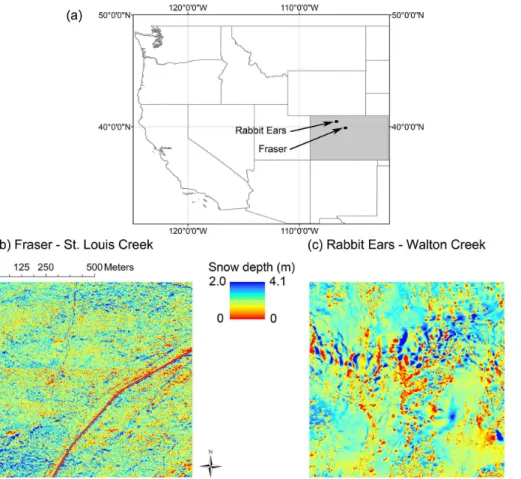
For the analyses and tests of the methodology introduced here, Light Detection and Ranging (LIDAR) snow depths obtained as part of the NASA’s Cold Land Processes Experiment (CLPX) will be used (Cline et al., 2009). The dataset consists of spatially distributed snow depths for 1 km×1 km areas (Intensive Study Areas – ISAs) in the

5

Colorado Rocky Mountains close to maximum snow accumulation in April 2003. For this study two areas will be used: the Fraser – St Louis Creek ISA (FS) and the Rabbit Ears – Walton Creek ISA (RW) (Fig. 1). The FS ISA is covered by a moderate density coniferous (lodgepole pine) forest on a flat aspect with low relief. The RW ISA is charac-terized by a broad meadow interspersed with small, dense stands of coniferous forest

10

and with low rolling topography. The snow depth distributions in these ISAs show diff er-ences that are relevant for the analysis of the methodology introduced here. At the FS ISA, the snow depth distribution is relatively isotropic (Fig. 1b), with short spatial corre-lation memory and little variations in the spatial scaling properties (i.e. power-spectral exponents and scaling breaks) with direction (Trujillo et al., 2007). On the other hand,

15

the spatial distribution of snow depth in the RW ISA is more anisotropic (Fig. 1c), with longer spatial correlation memory along a principal direction aligned with the predom-inant wind direction vs. shorter memory along the perpendicular direction, and with variations in the power-spectral exponents and scaling breaks according to the pre-dominant wind directions (Trujillo et al., 2007).

20

4 One-dimensional process

The spatial representation of the snow cover requires a basic assumption on the scale or resolution at which a field or profile is going to be represented at. This relies on the spatial support of the measurements. For the case of snow depths, point mea-surements from local surveys using a snow depth probe are frequently used for this

25

(9)

TCD

9, 1–44, 2015

Title Page

Tables Figures

◭ ◮

Back Close

Full Screen / Esc

Discussion

P

a

per

|

Discussion

P

a

per

|

Discussion

P

a

per

|

Discussion

P

a

per

|

these types of measurements, such as the accuracy of the position of the measure-ment in space or deviations in the vertical angle of penetration of the probe through the snow pack. These uncertainties are additional to any of the uncertainties estimated using the methodology discussed here.

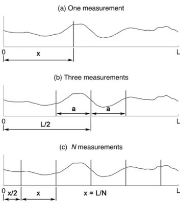
The one-dimensional case provides a good opportunity to illustrate the limitations of

5

point measurements. Consider the case of a snow depth profile that is measured using a snow depth probe at a regular spacing “d”. Each of these point measurements is meant to represent the mean snow depth over a particular distance surrounding the measurement, and the question is: over what distance is such assumption valid? In this case, the intrinsic assumption is that the measurement is representative over the

10

distance “d”, but at this point the validity of such assumption is not proven.

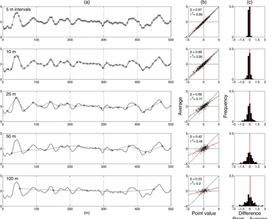
The answer to this question is conditioned to how variable the profile is and over what distances. To look at this, let us look at two snow depth profiles, one in a forested envi-ronment (FS) and another in an open envienvi-ronment (RW) in the Colorado Rocky Moun-tains (Figs. 2a and 3a, respectively). The variability in the profiles is markedly different,

15

with variations over shorter distances in the forested area, and a smoother profile in the open and wind influenced environment. This is reflected in the spatial correlation struc-ture of these snow depth profiles, with stronger correlations over longer distances in open and wind-influenced environments with respect to that in forested environments (Trujillo et al., 2007, 2009). These di_fferences should be considered when selecting

20

the sampling frequency required to capture the variability and accurately represent the mean conditions within a particular sampling spacing. This is illustrated by comparing the mean snow depth for a particular resolution to the point value at the center of the interval (Fig. 2b in a forested environment and Fig. 3b in an open and wind-influenced environment). In the Figures, average vs. point values at several sampling intervals are

25

(10)

TCD

9, 1–44, 2015

Title Page

Tables Figures

◭ ◮

Back Close

Full Screen / Esc

Discussion

P

a

per

|

Discussion

P

a

per

|

Discussion

P

a

per

|

Discussion

P

a

per

|

interval sizes. The degree of overestimation can be quantified through the slope of the regression line (in red in Figs. 2b and 3b). In the forested environment (Fig. 2b), the slopes range between 0.8 and 0.13, with decreasing slopes with increasing spacing. These slopes indicate that, on average, the mean values are 0.8 times the point values for the 5 m spacing and 0.1 times the point values for the 100 m spacing. In the open

5

and wind-dominated environment, the slopes are higher and range between 0.97 and 0.23 from 5 m spacing and 100 m spacing, respectively. A clear difference emerges: forested environments require shorter separation between single measurements if the snow depth profile is to be accurately captured by the measurements. The variability within the size of the interval determines the degree of uncertainty associated with the

10

point measurements, as the sub-interval variability is related to the degree of over-estimation of the mean value within the interval. Secondly, the differences between average and point values for each spacing distance are generally more scattered in the forested environment than in the open environment, and in both environments the degree of scattering increases with spacing (Figs. 2c and 3c). However, it is important

15

to note here that we are comparing normalized profiles (mean=0, SD=1), allowing us to focus on the rescaled spatial variations. What is highlighted is the relevance of the spatial structure of the profile rather than the absolute variance. This spatial structure can be quantified by, for example, the spatial covariance/correlation function.

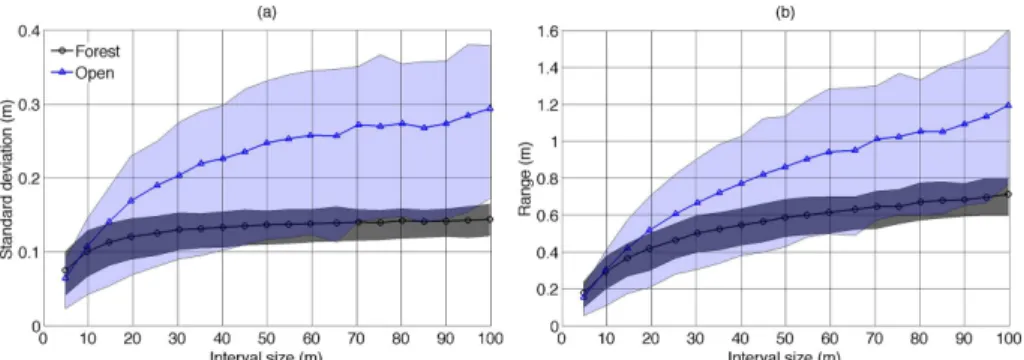
Additionally to the di_fferences in the correlation structure, there are also di_fferences

20

in the absolute variability in snow depth in these environments (Fig. 4). The subinterval SD as a function of interval size along the profiles is higher in the open and wind-influenced environment at RW vs. the forested environment at FS (Fig. 4a). Mean SD values in the open environment are twice as larger as those at the forested environment towards the larger interval sizes (∼100 m). The SD increases with interval size in both

25

(11)

TCD

9, 1–44, 2015

Title Page

Tables Figures

◭ ◮

Back Close

Full Screen / Esc

Discussion

P

a

per

|

Discussion

P

a

per

|

Discussion

P

a

per

|

Discussion

P

a

per

|

scales analyzed. Complementary, The shaded areas (25 to 75 % quantiles) give an idea of the variability of SD values, with a much wider range in RW vs. FS, and an increase in the range between quantiles with interval size in RW.

Also important, the sub-interval mean range (range defined as the difference be-tween the maximum and minimum snow depths within an interval) increases with

in-5

terval size in both FS and RW (Fig. 4b). However, the mean range is larger in the open environment at RW and the rate of increase with interval size is also steeper. Similarly, the shaded areas indicate wider distribution of range values in the open environment at RW, while relatively uniformly distributed around the mean across interval sizes in the forested environment at FS. The results in Figs. 2–4 illustrate two compensating

10

di_fferences between the snow covers in these environments and their influence on measurement strategies: that is, the forested environment requires shorter separation between measurements for accurate representation of the snow cover, however, in the wind-influence and open environment, the subinterval variability is higher indicating wider variations around any sampled measurement within the interval.

15

Ultimately, the number and distance between measurements and the specific ar-rangement of the measurements are all conditioned to what the measurements are needed for. Hydrologic applications may not require a highly detail representation of a snow depth profile (or a field), and representing the average conditions over a given distance (or area) is su_fficient, but small-scale process-based studies may require

20

a more detailed characterization over shorter distances (or smaller areas). This implies that the decision depends on the particular use that the measurements will support. In the following sections, the equations presented in the Background (Sect. 2) will be applied to evaluate the uncertainty associated with multiple measurement designs for profiles and fields of snow depth.

(12)

TCD

9, 1–44, 2015

Title Page

Tables Figures

◭ ◮

Back Close

Full Screen / Esc

Discussion

P

a

per

|

Discussion

P

a

per

|

Discussion

P

a

per

|

Discussion

P

a

per

|

4.1 Case 1: single measurement along a profile section

Equation (2) can be used to evaluate the uncertainty of a single measurement along a profile section of lengthL. For this case, as well as for the following cases in this article, an exponential covariance with a decay exponentν(ν >0) will be assumed:

C(h,σ,ν)=σ2_exp ₋_ν_k_h_k

forσ2_>_{0, and}_{ν >}₀ ₍₆₎

5

wereσ2is the variance, andkhkis the length of the vectorh. For this one-dimensional case and combining Eqs. (6) and (5), the following expression is obtained:

σ2

Z(x,L,ν) .

σ_p2=1− 2

Lν

2−exp(−νx)−exp(−ν·[L−x])

+ 1

L2_ν

2L+2

νexp(−νL)− 2 ν

(7)

wherexis the distance from one extreme of the section to the location of the

measure-10

ment (Fig. 5a). The normalized squared errorσ2

Z(x,L,ν)/σ

2

p is minimized atx equal to

half of the section length,L/2, regardless of ν. The existence of a correlation in the profile leads to this solution, as the middle location contains more information about the surroundings because of the correlation to the surrounding snow depths. Also, this solution is different from the solution for an uncorrelated profile (e.g. white noise), for

15

which the squared error would be equal to the variance, independent of the location of the measurement.

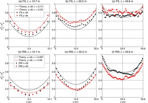
The results here are confirmed with an analysis of LIDAR snow depths profiles in FS and RW (Fig. 6). The analysis consists of calculating the difference between the mean and the point value for sections of a given length (varied between 10–50 m) and forx

20

(13)

TCD

9, 1–44, 2015

Title Page

Tables Figures

◭ ◮

Back Close

Full Screen / Esc

Discussion

P

a

per

|

Discussion

P

a

per

|

Discussion

P

a

per

|

Discussion

P

a

per

|

repeated for each section lengthL. The results indicate that the real snow depth profiles behave as predicted by the model of the error, with a minimum error atx equal to half of the section length. Another difference highlighted by these results is the difference between the sample errors in the forested environment (FS) vs. the open environment (RW) for the larger interval sizes (e.g. 50 m). The sampled normalized squared error

5

in the forested environment shows only a mild decrease in the square error to around 0.7–0.8 towards the inside of the section length. However, this decrease is achieved for the measurement along most of the interval length with the exception of the extremes. This can be explained by the relationship between the spatial memory of snow depth (e.g. the correlation function) and the section length. Densely forested environments

10

exhibit correlation lengths that are sorter than those in open and wind influenced en-vironments (e.g. Trujillo et al., 2007, 2009). As the section length increases beyond such correlation lengths, a measurement location towards the middle of the interval contains less information of the surrounding snow depths in a forested environment (e.g. FS) vs. an open and wind influenced environment (e.g. RW). This is observed

15

in Fig. 6c vs. Fig. 6f, with the results in RW showing a more clear minimum towards the center of the profile section. The results also show a poorer performance of the model in RW vs. FS, as the exponential correlation model has a poorer fit in RW at the shorter-lag range; however, model performance is improved for longer section lengths (e.g. Fig. 6c and f).

20

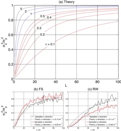
Model and sampled results thus support that the measurement location can be fixed in the middle of the interval, and the normalized squared error can then be described as a function of both, the exponential decay exponent,ν, and the length of the sec-tion, L (Fig. 7a). The normalized squared error increases with interval length, with a steeper increase for larger exponential decay exponents, for which the squared error

25

(14)

TCD

9, 1–44, 2015

Title Page

Tables Figures

◭ ◮

Back Close

Full Screen / Esc

Discussion

P

a

per

|

Discussion

P

a

per

|

Discussion

P

a

per

|

Discussion

P

a

per

|

lengthL. This is done for profiles separated every 30 m, similar to the analysis above, and for profiles along thex andy directions. The theoretical normalized squared error is estimated from Eq. (7) using the exponential decay exponent from the model fitted to the sampled correlation function. The results show that the theoretical model repro-duces the sampled squared error remarkably well, even reproducing the anisotropic

5

properties of the correlograms, represented by the different exponents of the exponen-tial model along x and y directions (Fig. 7b and c). The model also reproduces the different behavior of the squared error between both fields (i.e. FS and RW), showing that the normalized squared error increases more rapidly and is larger in the forested environment (Fig. 7b) vs. the open environment (Fig. 7c). However, it should be noted

10

here that as the error is normalized, and as the variance of the field in the open envi-ronment is larger (Fig. 4a), the absolute squared error could reach higher values in the open environment (RW). In this regard, one feature to discuss here is the assumption that the point variance of snow depth in these environments has been estimated as the spatial variance over the entire study area, as it is generally practiced in time

se-15

ries analysis and geostatistics. In practice, this is the only possible approach because there is limited information to estimate the point variance from multiple realizations of the process at each spatial location, as inter- and intra-annual snow depth fields are not available, not only for these areas, but for almost any area where this methodology may be applied.

20

4.2 Case 2: three measurement along a profile section

From Eq. (5) is also evident that increasing the number of measurements will reduce the squared error. In the case of three measurements separated by a distance “a”, with the middle measurement centered in the section of length L (Fig. 5b), and for an exponential covariance function with parameter ν, Eq. (5) leads to the following

25

(15)

TCD

9, 1–44, 2015

Title Page

Tables Figures

◭ ◮

Back Close

Full Screen / Esc

Discussion

P

a

per

|

Discussion

P

a

per

|

Discussion

P

a

per

|

Discussion

P

a

per

|

σ2

Z(a,L,ν) .

σ_p2=1

3+ 2 9 h

2 exp(−νa)−exp(−2νa)i

− 4

3Lν "

3−exp

−νL

2

(1+exp(−νa)+exp(νa)) #

+ 1

L2_ν

2L+2_νexp(−νL)−2

ν

.

(8)

Equation (8) can be minimized to determine the optimal separation distance between points,a, as a function ofLandν:

aoptimal=−

1

νln(t) (9)

where

5

t=B+

p

B2₋₄_AB

2A

A=4ν

9

and B=− 4

3Lexp

−νL

2

.

The combination of Eqs. (8) and (9) can be used to determine the normalized squared error,σ2

Z/σ

2

p, and the optimal distance,aoptimal, for the measurement pattern in Fig. 5b.

10

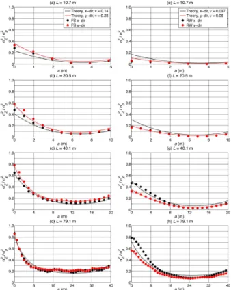
The model predicts that the normalized squared error is minimized at an intermediate location between 0 and L/2 (black lines in Fig. 8a and b). The results show an in-crease in the error with interval size,L, as well as little sensitivity ofaoptimal toν. This

latter feature can be seen as advantage since small biases in the estimation of νwill not result in significant biases in the estimation ofaoptimal. One could almost assume

(16)

TCD

9, 1–44, 2015

Title Page

Tables Figures

◭ ◮

Back Close

Full Screen / Esc

Discussion

P

a

per

|

Discussion

P

a

per

|

Discussion

P

a

per

|

Discussion

P

a

per

|

a value ofaoptimalwithout prior knowledge of the exponential decay exponent,

select-ing aoptimal within the range of values indicated by the model for a rage of possible

exponential decay exponents. Note thataoptimal is located close to the 60 % distance

from the center towards the outer boundary of the profile section for all section lengths (Fig. 8a and b). On the other hand, the measurement error displays a higher sensitivity

5

toνaroundaoptimal, indicating that biases in the estimation of toνwould have a more

noticeable effect on the estimation of the measurement error. This is further clarified in Fig. 8c, in which the normalized error (not squared) andaoptimalcan be obtained for

cor-responding profile section lengths (L) and exponential decay exponents (ν) based on the isolines shown. For example, for a profile section of 30 m, and an exponential decay

10

exponent of 0.2 m−1, the normalized error is 0.32 andaoptimalis 9.63 m (see intersect

of the two isolines in Fig. 8c). The normalized error in Fig. 8c is not squared, high-lighting the sensitivity of the measurement error toν, which represents the degree of spatial correlation of the profile in this case (e.g. lower values indicate stronger spatial memory/correlation, hence lower measurement errors).

15

The performance of the model is tested against the normalized squared error ob-tained from the same snow depth profiles in FS and RW. The test consists of estimating the normalized squared error for profiles sections of length between 10 and 80 m, with abeing varied between 0 andL/2 (Fig. 9). For each value ofa, the normalized squared error is estimated based on the means obtained using the three snow depth samples

20

for each section. All squared differences are then averaged to obtain the values pre-sented in the figure. Sampled and modeled errors follow the same trend across alla values and for the di_fferentLvalues in Fig. 9. The minimum error is also reproduced by the model proving the applicability of the model for estimating the optimal separation between measurements. The model does perform better in the forested environment

25

(17)

TCD

9, 1–44, 2015

Title Page

Tables Figures

◭ ◮

Back Close

Full Screen / Esc

Discussion

P

a

per

|

Discussion

P

a

per

|

Discussion

P

a

per

|

Discussion

P

a

per

|

of the snow depth distribution in this environment (higher spatial correlations) when compared to that in FS.

4.3 Case 3:N measurement along a profile section

As stated above, the measurement error can be reduced by increasing the number of measurements taken over a given section of lengthL. Let us focus on the case of

5

stratified sampling whereN regularly spaced measurements are taken over the inter-val (Fig. 5c), and to quantify this reduction we can use Eq. (5) and the exponential covariance model. Equation (5) can then be reduced to:

σ2

Z(N,L,ν)/σ

2

p=

1 N +

2 N2

N−1

X

k=1

kexp −ν

L−kL

N !

− 4

Lν "

1− 1

N N X

k=1

exp −νL N

N−k+1

2 !#

− 2

L2_ν2

1−Lν−exp(−νL) .

(10)

The normalized squared error (σ2 Z/σ

2

p) obtained with Eq. (10) for profiles sections of

10

lengths between 10 and 80 shows a steep decrease withN(Fig. 10), with a steeper de-crease for higher exponential decay exponents. For the longer profile sections (e.g. 80, Fig. 10d), little reductions are achieved in the squared error beyond only a few mea-surements (e.g. N=16). Equation (10) and the results in Fig. 10 can be used to de-termine the number of measurements necessary to achieve a desired accuracy level.

15

(18)

TCD

9, 1–44, 2015

Title Page

Tables Figures

◭ ◮

Back Close

Full Screen / Esc

Discussion

P

a

per

|

Discussion

P

a

per

|

Discussion

P

a

per

|

Discussion

P

a

per

|

intra-annual and inter-annual persistence of the spatial patterns, and hence, the spa-tial statistical properties of snow depth fields in mountain environments, as shown in previous studies using both manual surveys and LIDAR measurements (e.g. Deems et al., 2008; Schirmer et al., 2011; Melvold and Skaugen, 2013; Helfrich et al., 2014). A detailed spatial survey (e.g. dense manual measurements or TLS), sampling different

5

portions of an area can be used to determine the covariance/correlation characteristics of the snow depth distribution, with which the model for the error can be applied.

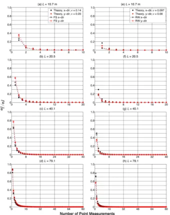
Following the method described in the previous section, we test the performance of the model against the normalized squared error obtained from the same snow depth profiles in FS and RW. In this case, the sampled squared error is estimated based on

10

theN regularly-spaced measurements distributed along the profile sections of length L. As the snow depth fields are gridded at ∼1 m resolution, the location of the mea-surements is approximated to the closest coordinate in the profile section following the pattern in Fig. 5c. Once again, sampled and modeled errors follow closely the same trend for the differentLvalues in both FS and RW (Fig. 11). The error decreases with

15

N, with a rapid decay at the lower N values, illustrating that the error can be drasti-cally reduced by simply increasing the number of measurements by a small amount. The normalized squared error across allN values is lower for RW than for FS, con-sistent with the higher spatial correlations observed in the snow depth fields of RW vs. FS. Once again, there are some di_fferences between the sampled and modeled

20

normalized squared error in RW for the shorter profile lengths and for smallN values: a consequence of the poorer fit of the exponential model for the shorter lag range in RW. However, the model is still able to reproduce the error in both fields, and the ap-plicability of the model is illustrated even when the fit of the correlation model can be improved.

(19)

TCD

9, 1–44, 2015

Full Screen / Esc

5 Two-dimensional process

Similar to the one-dimensional process, Eq. (5) can be formulated to calculate the squared error in the two-dimensional space. To exemplify this, we apply the method-ology to an isotropic process over the x−y plane for three cases in a square area: (a) one single measurement in the center of the area, (b) five measurements radiating

5

out from the center (Fig. 12a) and (c)N byN measurements regularly spaced in thex andy directions (Fig. 12b).

For the isotropic case, the covariance/correlation function is only dependent on the magnitude of the lag vector,

h_i,j =|xi−xj| (11)

10

and, consequently, the error is represented by,

σ2

Z(A)=σ

2 p             1 N + 2 N2

N−1

X

i=1

N X

j=i+1

CORR

h_i,j

− 2

NA N X

i=1

Z

A

CORR

h_i,j

dx_j

+ 1 A2 Z A Z A CORR

h_i,j

dx_idx_j             . (12)

The exponential correlation function for the isotropic case takes the following form:

(20)

TCD

9, 1–44, 2015

Full Screen / Esc

wherehis the magnitude of the lag vector. Replacing into the expression for σ2 Z, we obtain,

σ2 Z =σ

2 p             1 N + 2 N2

N−1

X

i=1

N X

j=i+1

exp −ν|x_i−x_j|

− 2

NA N X

i=1

Z

A

exp −ν|x_i−x_j| dx_j

+ 1 A2 Z A Z A

exp −ν|x_i−x_j| dx_jdx_i

            . (14)

For the case of a rectangular area of side dimensionLx andLy in the correspondingx andy directions, the equation becomes,

5

σ2 Z =σ

2 p               1 N + 2 N2

N−1

X

i=1

N X

j=i+1

exp−ν (x_i−x_j)2+(y_i−y_j)21₂

− 2

NA N X

i=1

Ly Z 0 Lx Z 0

exp−ν (xi−x)2+(yi−y)2 1₂

dxdy

+ 1 A2 Ly Z 0 L_x Z 0 Ly Z 0 L_x Z 0

exp−ν (x′−x)2+(y′−y)21₂

dxdydx′dy′               . (15)

The limits of the integrals can be changed depending on the desired location of the origin. In this case, the origin is located at the lower-left corner.

As discussed earlier, the first term is only a function of N, such that the base error is the variance of the point process divided by the number of points. The second term

10

(21)

TCD

9, 1–44, 2015

Title Page

Tables Figures

◭ ◮

Back Close

Full Screen / Esc

Discussion

P

a

per

|

Discussion

P

a

per

|

Discussion

P

a

per

|

Discussion

P

a

per

|

a function ofN,A, the location of the points, and the decay rate ν. The fourth term is a function of Aand ν, but is independent of the location of the points and N (i.e. in-dependent of the survey design, and only a function of the correlation structure of the continuous process).

5.1 Case 1: single measurement in the center of the area 5

In this case, we focus on a single measurement in the middle of a square area of side dimensionL. Numerical solution of Eq. (15) shows that the normalized squared error increases rapidly with L, with a steeper increase for higher exponential decay expo-nents (Fig. 13a), which approach a normalized squared error of 1 for L values less than 10 (e.g. 1≤ν≤5). The theoretical results in Fig. 13a can be used to determine

10

the discrepancy between a single measurement in the middle of an area and the areal mean for a second order stationary and anisotropic process with an exponential covari-ance/correlation function. Comparison of the modeled and sampled normalized square errors for the FS snow depth field indicate very good agreement between modeled and sample errors (Fig. 13b). The sample error is estimated following the same procedure

15

explained for the one-dimensional cases, although in the two-dimensional space. Both sampled and modeled errors show the same behavior acrossLvalues between 1 and 100 m, although the scatter in the sampled error increases for larger L values. This can be explained by the smaller number of samples to estimate the mean normalized squared error and the fact that the correlation structure decays rapidly and a single

20

(22)

TCD

9, 1–44, 2015

Title Page

Tables Figures

◭ ◮

Back Close

Full Screen / Esc

Discussion

P

a

per

|

Discussion

P

a

per

|

Discussion

P

a

per

|

Discussion

P

a

per

|

5.2 Case 2: five measurements radiating out from the center of the area

The case five measurements radiating out from the center (Fig. 12a), with a point in the middle of the area and four points separated by a distanceafrom the center leads to a solution that allows for the optimization problem illustrated in case 2 of the one-dimensional examples (Sect. 4.2). In the two-one-dimensional case, Eq. (15) does not have

5

an explicit solution fora, and numerical implementation is required. The equation can be solved by simply replacing the point coordinates and the correlation function param-eters. Following this approach, the normalized squared error can be obtained for areas of varying sizes (Fig. 14). Similar to the one-dimensional example (case 2, Sect. 4.2), σ2

Z/σ

2

p decreases with a, reaching a minimum at an intermediate distance from the

10

middle point outwards. The decay inσ2 Z/σ

2

p is more rapid for the least correlated

pro-cesses (i.e. higher decay exponents) reaching a value close to the base normalized square error that is a function of the number of points (i.e. 1/N=1/5 in this case). An extended analysis of the effect of each of the terms in the equation is included in the Supplement (Part I). The error, as shown in Fig. 14, is minimized as a consequence

15

of two balancing terms that lead to this intermediate solution. The optimal solution is a balance between reducing the correlation between the individual measurements (e.g. increasing the separation between the location of the measurements) but increas-ing the correlation between the measurements and the surroundincreas-ing area (e.g. locatincreas-ing the measurements closer to the middle of the area). These two competing effects lead

20

to an optimization problem based on the location of the point measurements. For the least correlated processes, the error behaves closer to the behavior of an uncorrelated field once the measurements become effectively decorrelated (e.g.a >1 in Fig. 14b for ν=5). Figure 14 exemplifies how Eq. (15) can be used to determine the optimal mea-surement location for areas of different sizes, and to determine the associated error

25

with configurations other than the optimal.

(23)

TCD

9, 1–44, 2015

Title Page

Tables Figures

◭ ◮

Back Close

Full Screen / Esc

Discussion

P

a

per

|

Discussion

P

a

per

|

Discussion

P

a

per

|

Discussion

P

a

per

|

squared error for square areas of side dimension (L) between 10 and 79 m, withabeing varied between 0 andL/2 (Fig. 15). For each value ofa, the normalized squared error is estimated based on the means obtained using the five snow depth samples for each section. All squared differences are then averaged to obtain the values presented in the figure. Once again, the sampled and modeled errors follow the same trend across all

5

avalues and for the differentL values. The minimum error andaoptimalare also

repro-duced closely by the model, and as the area size increases, the sampled and modeled error approach the error for an uncorrelated field at larger separations (i.e. 0.2). These results illustrate that the performance of the model in the two-dimensional space is remarkable, similar to what was observed in the one-dimensional case.

10

5.3 Case 3:N byNmeasurements regularly spaced in thexandy directions

Similarly to the one-dimensional case, the two-dimensional case ofN byN regularly spaced measurements (Fig. 12b) leads to a decreasing normalized squared error with N (Fig. 16). There is a sharp decrease in the error with just increasing the number of measurements in the lower range ofN. The analysis illustrates that stratified sampling,

15

as the one shown here, is an excellent approach to minimizing the error. For example, for the area of 10 by 10, increasingN to 4 (N2=16) reduces the normalized squared error to less than 0.05. It is also worth noting here that for this two-dimensional case, the error is less sensitive to the value of the exponential decay exponent (ν) for the higher N values as the mean is accurately captured regardless of the correlation of

20

the field. Figure 16 serves as an example of how the methodology can be used for objective selection of the number of measurements necessary to achieve a desired accuracy level using prior knowledge of the spatial covariance function.

The performance of the model is tested again for square areas of side dimension (L) between 10 and 79 m using the snow depth field in FS, and for an increasing

num-25

(24)

TCD

9, 1–44, 2015

Title Page

Tables Figures

◭ ◮

Back Close

Full Screen / Esc

Discussion

P

a

per

|

Discussion

P

a

per

|

Discussion

P

a

per

|

Discussion

P

a

per

|

sampled and modeled errors increase as the size of the area increases, as expected. These results complete the model performance tests for the two-dimensional isotropic case.

6 Summary and conclusions

A methodology for an objective evaluation of the error in capturing mean snow depths

5

from point measurements is presented based on the expected value of the squared difference between the real average snow depth and the mean of a finite number of snow depth samples within a defined domain (e.g. a profile section or an area). The model can be used for assisting the design of survey strategies such that the error is minimized in the case of a limited and predetermined number of measurements, or

10

such that the desired number of measurements is determined based on a predefined acceptable uncertainty level. The model is applied to one- and two-dimensional survey examples using LIDAR snow depths collected in the Colorado Rockies. The results confirm that the model is capable of reproducing the estimation error of the mean from a finite number of samples for real snow depth fields. The theoretical framework

15

introduced here requires knowledge of certain spatial statistical properties (e.g. best covariance/correlation model and parameters, as illustrated here using the exponential correlation model with parameterν). These properties are also shared by other spatially heterogeneous fields and processes that are hydrologically-relevant, such as snow water equivalent, soil moisture and precipitation, among others. In consequence, this

20

methodology can be extended to the aforementioned variables and processes.

Currently, remote sensing technologies (e.g. TLS, Airborne LiDAR, and Ground Pen-etrating Radar) are allowing for the characterization of snow cover properties at in-creasing resolutions in both space and time. Such improvements can be utilized in the context introduced here to optimize survey design such that estimation errors can be

25

(25)

TCD

9, 1–44, 2015

Title Page

Tables Figures

◭ ◮

Back Close

Full Screen / Esc

Discussion

P

a

per

|

Discussion

P

a

per

|

Discussion

P

a

per

|

Discussion

P

a

per

|

will continue to be relevant despite of the aforementioned improvements, as access to these technologies is limited by their cost and the expertise that is required for their application.

The Supplement related to this article is available online at doi:10.5194/tcd-9-1-2015-supplement.

5

Acknowledgements. Data for this article was obtained from NASA’s Cold Land Processes ex-periment (CLPX), available at http://nsidc.org/data/docs/daac/nsidc0157_clpx_lidar.

References

Blöschl, G.: Scaling issues in snow hydrology, Hydrol. Process., 13, 2149–2175, 1999.

Chang, A. T. C., Kelly, R. E. J., Josberger, E. G., Armstrong, R. L., Foster, J. L., and

Mog-10

nard, N. M.: Analysis of ground-measured and passive-microwave-derived snow depth variations in midwinter across the northern Great Plains, J. Hydrometeorol., 6, 20–33, doi:10.1175/Jhm-405.1, 2005.

Cline, D., Yueh, S., Chapman, B., Stankov, B., Gasiewski, A., Masters, D., Elder, K., Kelly, R., Painter, T. H., Miller, S., Katzberg, S., and Mahrt, L.: NASA cold land processes experiment

15

(CLPX 2002/03): airborne remote sensing, J. Hydrometeorol., 10, 338–346, 2009.

Deems, J. S., Fassnacht, S. R., and Elder, K. J.: Interannual consistency in fractal snow depth patterns at two Colorado mountain sites, J. Hydrometeorol., 9, 977–988, doi:10.1175/2008jhm901.1, 2008.

Grünewald, T. and Lehning, M.: Are flat-field snow depth measurements representative? A

com-20

parison of selected index sites with areal snow depth measurements at the small catchment scale, Hydrol. Process., doi:10.1002/hyp.10295, in press, 2014.

Helfrich, K., Schöber, J., Schneider, K., Sailer, R., and Kuhn, M.: Interannual persis-tence of the seasonal snow cover in a glacierized catchment, J. Glaciol., 60, 889–904, doi:10.3189/2014JoG13J197, 2014.

25

(26)

TCD

9, 1–44, 2015

Title Page

Tables Figures

◭ ◮

Back Close

Full Screen / Esc

Discussion

P

a

per

|

Discussion

P

a

per

|

Discussion

P

a

per

|

Discussion

P

a

per

|

López-Moreno, J. I., Fassnacht, S. R., Beguería, S., and Latron, J. B. P.: Variability of snow depth at the plot scale: implications for mean depth estimation and sampling strategies, The Cryosphere, 5, 617–629, doi:10.5194/tc-5-617-2011, 2011.

Melvold, K. and Skaugen, T.: Multiscale spatial variability of lidar-derived and modeled snow depth on Hardangervidda, Norway, Ann. Glaciol., 54, 273–281, 2013.

5

Meromy, L., Molotch, N. P., Link, T. E., Fassnacht, S. R., and Rice, R.: Subgrid variability of snow water equivalent at operational snow stations in the western USA, Hydrol. Process., 27, 2383–2400, doi:10.1002/Hyp.9355, 2013.

Mott, R., Schirmer, M., and Lehning, M.: Scaling properties of wind and snow depth distribution in an alpine catchment, J. Geophys. Res.-Atmos., 116, D06106, doi:10.1029/2010JD014886,

10

2011.

Rice, R. and Bales, R. C.: Embedded-sensor network design for snow cover measurements around snow pillow and snow course sites in the Sierra Nevada of California, Water Resour. Res., 46, W03537, doi:10.1029/2008wr007318, 2010.

Rodríguez-Iturbe, I. and Mejía, J. M.: Design of rainfall networks in time and space, Water

15

Resour. Res., 10, 713–728, 1974.

Schirmer, M., Wirz, V., Clifton, A., and Lehning, M.: Persistence in intra-annual snow depth distribution: 1. Measurements and topographic control, Water Resour. Res., 47, W09516, doi:10.1029/2010WR009426, 2011.

Shea, C. and Jamieson, B.: Star: An efficient snow point-sampling method, Ann. Glaciol., 51,

20

64–72, 2010.

Skøien, J. O. and Blöschl, G.: Sampling scale effects in random fields and implications for environmental monitoring, Environ. Monit. Assess., 114, 521–552, doi:10.1007/S10661-006-4939-Z, 2006.

Trujillo, E., Ramirez, J. A., and Elder, K. J.: Topographic, meteorologic, and canopy controls

25

on the scaling characteristics of the spatial distribution of snow depth fields, Water Resour. Res., 43, W07409, doi:10.1029/2006WR005317, 2007.

Trujillo, E., Ramírez, J. A., and Elder, K. J.: Scaling properties and spatial organization of snow depth fields in sub-alpine forest and alpine tundra, Hydrol. Process., 23, 1575–1590, doi:10.1002/hyp.7270, 2009.

30

(27)

TCD

9, 1–44, 2015

Title Page

Tables Figures

◭ ◮

Back Close

Full Screen / Esc

Discussion

P

a

per

|

Discussion

P

a

per

|

Discussion

P

a

per

|

Discussion

P

a

per

|

(28)

TCD

9, 1–44, 2015

Title Page

Tables Figures

◭ ◮

Back Close

Full Screen / Esc

Discussion

P

a

per

|

Discussion

P

a

per

|

Discussion

P

a

per

|

Discussion

P

a

per

|

(29)

TCD

9, 1–44, 2015

Title Page

Tables Figures

◭ ◮

Back Close

Full Screen / Esc

Discussion

P

a

per

|

Discussion

P

a

per

|

Discussion

P

a

per

|

Discussion

P

a

per

|

(30)

TCD

9, 1–44, 2015

Title Page

Tables Figures

◭ ◮

Back Close

Full Screen / Esc

Discussion

P

a

per

|

Discussion

P

a

per

|

Discussion

P

a

per

|

Discussion

P

a

per

|

Figure 3. (a)As Fig. 2 but for an open and wind influenced environment at the Rabbit Ears – Walton Creek (RW) ISA of the CLPX (Trujillo et al., 2007; Cline et al., 2009).(b)Average values within sampling intervals (same as ina) vs. point samples for normalized snow depth profiles in the RW ISA. The red line is a linear regression fit, with slopeβandr2as indicated in each plot.

(31)

TCD

9, 1–44, 2015

Title Page

Tables Figures

◭ ◮

Back Close

Full Screen / Esc

Discussion

P

a

per

|

Discussion

P

a

per

|

Discussion

P

a

per

|

Discussion

P

a

per

|

(32)

TCD

9, 1–44, 2015

Title Page

Tables Figures

◭ ◮

Back Close

Full Screen / Esc

Discussion

P

a

per

|

Discussion

P

a

per

|

Discussion

P

a

per

|

Discussion

P

a

per

|

(33)

TCD

9, 1–44, 2015

Title Page

Tables Figures

◭ ◮

Back Close

Full Screen / Esc

Discussion

P

a

per

|

Discussion

P

a

per

|

Discussion

P

a

per

|

Discussion

P

a

per

|

Figure 6.Comparison of the theoretical and sampled normalized squared error (σ2

Z/σ

2

p) for the

(34)

TCD

9, 1–44, 2015

Title Page

Tables Figures

◭ ◮

Back Close

Full Screen / Esc

Discussion

P

a

per

|

Discussion

P

a

per

|

Discussion

P

a

per

|

Discussion

P

a

per

|

Figure 7. (a)Theoretical normalized squared error for a single measurement in the middle of a section of length, L, and for an exponential correlation function with a decay exponent,