An optimised method for correcting quenched fluorescence yield

(1)

OSD

11, 1243–1264, 2014

An optimised method for correcting

quenched fluorescence yield

L. Biermann et al.

Title Page

Abstract Introduction

Conclusions References

Tables Figures

◭ ◮

Back Close

Full Screen / Esc

Printer-friendly Version Interactive Discussion

Discussion

P

a

per

|

D

iscussion

P

a

per

|

Discussion

P

a

per

|

Discuss

ion

P

a

per

|

Ocean Sci. Discuss., 11, 1243–1264, 2014 www.ocean-sci-discuss.net/11/1243/2014/ doi:10.5194/osd-11-1243-2014

Open Access

Ocean Science

Discussions

This discussion paper is/has been under review for the journal Ocean Science (OS). Please refer to the corresponding final paper in OS if available.

An optimised method for correcting

quenched fluorescence yield

L. Biermann1, C. Guinet2, M. Bester3, A. Brierley4, and L. Boehme1

1

Sea Mammal Research Unit, Scottish Oceans Institute, St. Andrews, UK

2

Centre National de la Recherche Scientifique, Centre d’Etudes Biologiques de Chizé Villiers en Bois, France

3

Mammal Research Institute, Department of Zoology and Entomology, University of Pretoria, South Africa

4

Pelagic Ecology Research Group, Scottish Oceans Institute, St. Andrews, UK

Received: 8 April 2014 – Accepted: 22 April 2014 – Published: 9 May 2014

Correspondence to: L. Biermann (lb66@st-andrews.ac.uk)

(2)

OSD

11, 1243–1264, 2014

L. Biermann et al.

Title Page

Tables Figures

◭ ◮

Back Close

Full Screen / Esc

Discussion

P

a

per

|

D

iscussion

P

a

per

|

Discussion

P

a

per

|

Discuss

ion

P

a

per

|

Abstract

Under high light intensity, phytoplankton protect their photosystems from bleaching through non-photochemical quenching processes. The consequence of this is sup-pression of fluorescence emission, which must be corrected when measuring in situ yield with fluorometers. Previously, this has been done using the limit of the mixed 5

layer, assuming that phytoplankton are uniformly mixed from the surface to this depth. However, the assumption of homogeneity is not robust in oceanic regimes that support deep chlorophyll maxima. To account for these features, we correct from the limit of the euphotic zone, defined as the depth at which light is at∼1 % of the surface value. This

method was applied to fluorescence data collected by eleven animal-borne fluorome-10

ters deployed in the Southern Ocean over four austral summers. Six tags returned data showing evidence of deep chlorophyll features. Using the depth of the euphotic layer, quenching was corrected without masking subsurface fluorescence signals.

1 Introduction

Monitoring distribution and abundance of primary producers in the marine environment 15

is useful for understanding larger physical and environmental processes. Phytoplank-ton are predominantly single-celled, green microscopic organisms; present at variable concentrations in every ocean (Falkowski and Kolber, 1995; Behrenfeld et al., 2009). They are the first stepping-stone in transferring energy into the marine ecosystem. When conditions allow for growth, their collective impact is such that they are able to 20

change the spectral properties of the water (McClain, 2009). This can be exploited to measure abundance and distribution using their photosynthetic pigment, chloro-phylla(Chla) as a marker (Morel and Prieur, 1977; Gordon and Morel, 1983; Falkowski et al., 1998; Henson et al., 2010).

Satellite-derived ocean colour is the most comprehensive dataset available for mon-25

(3)

OSD

11, 1243–1264, 2014

L. Biermann et al.

Title Page

Tables Figures

◭ ◮

Back Close

Full Screen / Esc

Discussion

P

a

per

|

D

iscussion

P

a

per

|

Discussion

P

a

per

|

Discuss

ion

P

a

per

|

significant (Dierssen and Smith, 2000; McClain, 2009). Perhaps most significantly, satellite sensors can only “see” ocean colour from the surface to one optical depth; providing little information on the vertical structure of the water column (Morel and Berthon, 1989). Despite innovative algorithms to improve data collected by satellites, limitations are not likely to be resolved with the next generation of ocean colour sen-5

sors. Continued collection of in situ data on phytoplankton distribution and abundance is thus essential (Johnson et al., 2009).

Fluorescence has been widely used as a relatively inexpensive, non-invasive method for studying phytoplankton and quantifying Chl a since the 1960’s (Lorenzen, 1966; Lorenzen and Jeffrey, 1980; Cullen and Eppley, 1981; Falkowski and Kolber, 1995; Xing 10

et al., 2011; Lavigne et al., 2012). Chlorophyll pigments packaged inside phytoplankton cells re-radiate∼2 % of light energy as fluorescence. Active fluorescence can thus be

measured by a fluorometer delivering voltage output equivalent to 460 nm (excitation in the blue) and measuring resultant fluorescence in the 620–715 nm range (detection in the red). Assuming that the measured yield is proportional to the abundance of pho-15

tosynthesising phytoplankton, relative values of fluorescence can be used to quantify primary biomass. However, yield (and thus proportionality) is a_ffected by several fac-tors, including the intensity of sunlight each cell is exposed to (Behrenfeld and Boss, 2006).

To regulate high sunlight intensity, phytoplankton employ the mechanism of non-20

photochemical quenching. This process helps cells protect themselves in environments where light energy absorption exceeds the capacity for light utilisation (Müller et al., 2001; Behrenfeld et al., 2009). During periods of high light stress, shallow-mixed phy-toplankton in the upper euphotic layer protect their photosystems from bleaching by emitting excess energy as heat (Milligan et al., 2012). In this state of photo-protection, 25

(4)

OSD

11, 1243–1264, 2014

L. Biermann et al.

Title Page

Tables Figures

◭ ◮

Back Close

Full Screen / Esc

Discussion

P

a

per

|

D

iscussion

P

a

per

|

Discussion

P

a

per

|

Discuss

ion

P

a

per

|

shallow-mixed biomass will be “invisible” to a fluorometer. If uncorrected, quenched fluorescence yields will generate surface values under-representative of phytoplankton abundance. Avoiding such under-representation is particularly important for studies comparing satellite-derived surface Chlawith in situ fluorescence derived Chla.

On the vertical scale, quenched fluorescence profiles are also problematic in that 5

they have the same shape as deep fluorescence maxima (DFM). Sub-surface fluores-cence maxima can be indicative of deep chlorophyll maxima (DCM), which form when the bulk of phytoplankton biomass settles to depths where both nutrients and light are sufficient (Cullen and Eppley, 1981; Holm-Hansen and Hewes, 2004). Because DCM are usually found below one optical depth, abundance and distribution of such features 10

cannot be measured by satellite (McClain, 2009; Charrassin et al., 2010). However, DCM play important roles in the organisation of pelagic trophic food webs, as well as underreported roles in contributing to net primary production and carbon fixation (Fair-banks et al., 1982; Estrada et al., 1993; Claustre et al., 2008). It is therefore necessary to accurately identify and map these features.

15

In previous work on glider data, correcting for quenching involved using backscat-ter (Sackmann, 2008) or surface light intensity (Todd et al., 2009); each measured simultaneously to fluorescence. For autonomous platforms collecting “only” fluores-cence, salinity and temperature data, this is not possible. Using the depth of the density-derived mixed layer, Xing et al. (2011) corrected quenched fluorescence data 20

collected by Argo floats in Pacific, Atlantic, and Mediterranean offshore zones. This mixed layer depth (MLD) method was then extended to fluorescence data collected by tagged southern elephant seals (Mirounga leonina) o_ff Kerguelen Island in the Southern Ocean (Xing et al., 2012; Guinet et al., 2013). Following the method of Xing et al. (2011), the maximum fluorescence yield within the density-derived mixed layer 25

(5)

OSD

11, 1243–1264, 2014

L. Biermann et al.

Title Page

Tables Figures

◭ ◮

Back Close

Full Screen / Esc

Discussion

P

a

per

|

D

iscussion

P

a

per

|

Discussion

P

a

per

|

Discuss

ion

P

a

per

|

is especially true for motile (flagellated) and seasonally successive (heavily silicified) species (Mengesha et al., 1998; Quéguiner, 2013).

In this paper, we present a method to correct for quenching using the limit of the eu-photic zone (Z_eu), defined as the depth at which light is at∼1 % of the surface value. At

this level, light should be sufficient for photosynthesis but too weak to cause quenching. 5

This method is applied to fluorescence data collected by 11 animal-borne fluorometer, conductivity, temperature and depth satellite-relayed data loggers (FCTD-SRDLs) de-ployed in the Southern Ocean over several austral summers. Surface waters of this oceanic regime are well-mixed and DCM are thought to be rare. However, a southern elephant seal tagged on Marion Island travelled to a region correctly hypothesised to 10

support sub-surface features (Holm-Hansen et al., 2005). Animals tagged on Kergue-len Island also returned fluorescence profiles exhibiting deep features.

2 Methods

2.1 In-situ data

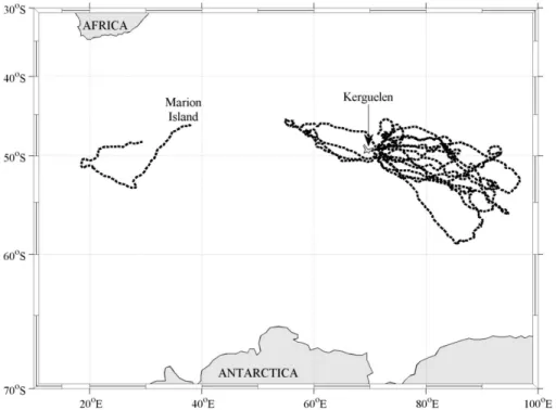
Between 2009 and 2013 ten adult female southern elephant seals from Kerguelen and 15

one from Marion Island were equipped with FCTD-SRDLs (Sea Mammal Research Unit, St Andrews University, Scotland) before they undertook their post-breeding forag-ing migration over the austral summer (Fig. 1). Followforag-ing established taggforag-ing protocols (Bester, 1988; McIntyre et al., 2010), the seal on Marion Island was immobilized with ketamine using a remote injection method and the tag was glued to the fur on the 20

head with quick-setting epoxy resin. Seals on Kerguelen were anesthetised with an intravenous injection of tiletamine and zolazepam 1 : 1 and tags were glued to the fur on the head using a two component industrial epoxy (Araldite AW 2101) (Jaud et al., 2012).

The FCTD-SRDL instrument records behavioural data as well as in situ pressure, 25

(6)

OSD

11, 1243–1264, 2014

L. Biermann et al.

Title Page

Tables Figures

◭ ◮

Back Close

Full Screen / Esc

Discussion

P

a

per

|

D

iscussion

P

a

per

|

Discussion

P

a

per

|

Discuss

ion

P

a

per

|

At-sea data were relayed via the Argos satellite system (http://www.argos-system.org). Location estimates were calculated by Service Argos from Doppler Shift measure-ments between uplinks and raw data were downloaded from the Sea Mammal Re-search Unit (SMRU) website (http://www.smru.st-andrews.ac.uk/). Detailed information on the hardware and software of the CTD-SRDL is described by Boehme et al. (2009), 5

and on-board data processing is described comprehensively by Fedak et al. (2002). Fluorescence is recorded by a Cyclops 7 fluorometer (Turner Designs, CA, USA), which delivers a voltage output proportional to the fluorescence detected in a wave-length between 620 and 715 nm. The Cyclops instrument is programmed to measure fluorescence every 2 s during the ascent (upcast), from 180 m to the surface. Due to the 10

tight limits on data transfer through the Argos satellite system, fluorescence data have to be compressed (Boehme et al., 2009) into 10 m vertical bins. The reading for “175 m” is thus a weighted mean of all fluorescence readings taken between 180 m and 170 m. This is the deepest bin available – deep and dark enough to anticipate an absence of live, photosynthesising phytoplankton (Guinet et al., 2013). However, instruments do 15

not return readings of zero at these depths. This “dark count” is an offset value added by the manufacturers; useful because at very low signal, readings are indistinguishable from noise. The offset value increases the signal to noise ratio, which must be removed during data processing (Lavigne et al., 2012). We therefore calculated the mean of readings at 175 m and subtracted this from all measurements collected by the same 20

tag (Xing et al., 2011). This is not only useful for making the fluorescence values more representative, it also serves to reduce variability between tags (Xing et al., 2012). The resulting values are considered proportional to fluorescence, and are termed Relative Fluorescence Units (RFU).

2.2 Satellite data

25

(7)

OSD

11, 1243–1264, 2014

L. Biermann et al.

Title Page

Tables Figures

◭ ◮

Back Close

Full Screen / Esc

Discussion

P

a

per

|

D

iscussion

P

a

per

|

Discussion

P

a

per

|

Discuss

ion

P

a

per

|

of the water-leaving radiance by the Moderate Imaging Spectrometer (MODIS) as 4×

4 km monthly composites (http://oceancolor.gsfc.nasa.gov).

MODIS provides two products ofZ_eu from remotely derived ocean colour (Lee et al., 2007; Morel, 1988; Morel et al., 2007). Morel’s Chl-approach is an empirical method centred on the assumption that the optical properties of the water are “only” affected 5

by Chl a (Case-1 waters). The calculation of Z_eu is thus solely based on remotely-sensed Chl a concentration. Lee’s IOP-approach, on the other hand, is derived with the addition of inherent optical properties (IOPs). Knowledge ofZ_euthus requires infor-mation on backscattering and absorption coefficients at 490 nm (Shang et al., 2011). While open waters of the Southern Ocean likely conform to case-1 assumptions (Soppa 10

et al., 2013), Lee’s approach was selected because the addition of IOPs are potentially beneficial for improved accuracy and reliability (Dierssen and Smith, 2000).

For adequate temporal and spatial coverage in a region as cloudy as the Southern Ocean, monthly composites ofZ_eu were favoured over 8 day. Basic correlations were applied to test reliability of the monthly product against the 8 day product. Good agree-15

ment between the two supported the decision to use monthly composites (n₌480, R2₌0.82, p <0.0001). However, despite the broad coverage in time, gaps were still present in space. For each fluorometer profile the closestZ_eu value in space was ex-tracted from the gridded dataset. If no value was available,Z_euwas interpolated linearly from the nearest seal position with an associatedZ_euvalue.

20

2.3 Correcting for quenching

In this study, we compare the results of fluorescence quenching correction from two depths. The first is the depth of Z_eu using Lee’s algorithm (2007). The second is a density-derived MLD calculated from the concurrent CTD measurements of the FCTD-SRDL. Here, MLD is defined as the depth where the vertical density gradient 25

equals or exceeds a threshold value (Kara et al., 2000). To date, a range of thresholds have been used in the literature; from the most sensitive of 0.005 kg m−3_{(e.g. Brainerd}

(8)

OSD

11, 1243–1264, 2014

L. Biermann et al.

Title Page

Tables Figures

◭ ◮

Back Close

Full Screen / Esc

Discussion

P

a

per

|

D

iscussion

P

a

per

|

Discussion

P

a

per

|

Discuss

ion

P

a

per

|

0.15 kg m−3 _{(e.g. Lewis et al., 1990; Weller and Plueddemann, 1996). Visual}

inspec-tion of the density along seal tracks supported a threshold of∆ρ₌0.03 kg m−3_{, which}

is small enough to not increase a mixed-layer heat budget (Dong et al., 2008), while also accounting for all possible uncertainties within the derived density profiles.

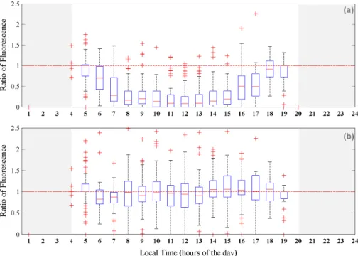
Quenching occurs in surface waters during periods of high light stress. Despite daily 5

variability attributed to cloud (changing light intensity), and di_fferences in phytoplankton concentrations between years and regions, suppression of fluorescence is a ubiquitous feature. Fitting a non-linear model (sin-function) to surface fluorescence as a function of time of day showed that quenching around midday was significant (n₌1267,R2₌ 0.26, P <0.001) (Fig. S1). Data were thus categorised as “day: possibly quenched” 10

(from sunrise to sunset, with the sun 6◦ _{above the horizon) or “night: unquenched”. To}

illustrate the quenching e_ffect without interannual and regional variability, “day” yields were divided by the preceding “night” yields to generate ratios. Data were then binned by hour and plotted using boxplots (Fig. 2).

To find deep fluorescence features, the “night: unquenched” data were normalised 15

and each profile was interrogated for maximum values below the near-surface yield. For this step, the small proportion of profiles with maximum fluorescence yields be-low 0.15 RFU were removed from the dataset. These be-low signals tend to fall within the noise, and the resulting vertical profiles cannot be meaningfully interpreted. Remaining profiles exhibiting a deep fluorescence yield of 15 % or higher than the near-surface 20

fluorescence were then visually inspected. Vertical profiles conforming to the shape of DFM in this dataset were considered “true” DFM, independent of quenching (Fig. S2). The “day: quenched” data were corrected using bothZ_eu and MLD; creating two sepa-rate subsets for comparison. In both cases, the maximum fluorescence yield between Z_eu and the surface, or MLD and the surface, was then extended to fill in supressed 25

(9)

OSD

11, 1243–1264, 2014

L. Biermann et al.

Title Page

Tables Figures

◭ ◮

Back Close

Full Screen / Esc

Discussion

P

a

per

|

D

iscussion

P

a

per

|

Discussion

P

a

per

|

Discuss

ion

P

a

per

|

3 Results

The at-sea phases of the eleven tagged southern elephant seals (Fig. 1) tended to start in November and end in January of the following year, meaning data were collected over the height of the austral summer. In the top 10–15 m of the upper mixed layer across all years of sampling, suppression of daytime fluorescence yield was significant. 5

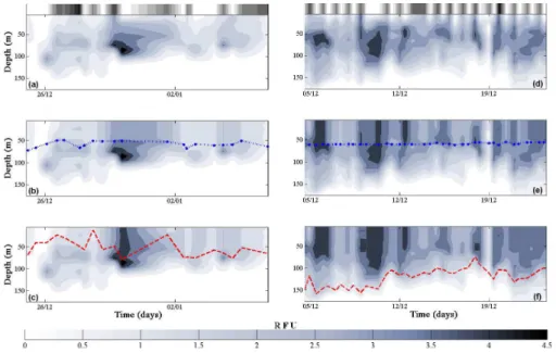
To correct for this, surface values collected between dawn and dusk were “filled in” with maximum values from the depth ofZ_eu. For comparative analysis, the same data were then corrected from the depth of the mixed layer. The difference between the two methods is illustrated in Fig. 3, where normalised fluorescence profiles were treated with both correction schemes. UsingZ_euprevents the distinct deep features from being 10

masked in all cases.

Applying the two different correction schemes does not always result in significant differences in yield at the surface; however correcting from Z_eu serves to conserve “unusual” (not homogenously mixed) phytoplankton dynamics on the vertical scale. This is illustrated in Fig. 3d and e where the shallow- and deep-mixed phyotoplankton 15

appear to have settled into two distinct layers. Corrected surface fluorescence yields are only negligibly overestimated using the depth of the mixed layer; but perhaps more importantly, vertical complexity is lost.

Of the eleven seals tagged with FCTD-SRDLs between 2009 and 2013, only one instrument returned data completely absent of subsurface fluorescence maxima. For 20

the remaining ten “night: unquenched” datasets, approximately 24 % (Std. Dev.=16) of the 231 profiles showed “true” DFM (Fig. S2).

One seal was tagged on Marion Island in 2012 as part of an initiative to search for DFM in a region hypothesised to support DCM (approximately 20◦_{E to 20}◦_{W, 57 to}

60◦_{S) (Holm-Hansen et al., 2005). We extended this region to the limit of the Polar}

25

Front at around 50◦_{S (Orsi and Ryan, 2001) after reviewing the physics of the}

re-gion. The tagged seal entered this extended region (20◦_{E to 20}◦_{W, 50 to 60}◦_{S) and}

(10)

OSD

11, 1243–1264, 2014

L. Biermann et al.

Title Page

Tables Figures

◭ ◮

Back Close

Full Screen / Esc

Discussion

P

a

per

|

D

iscussion

P

a

per

|

Discussion

P

a

per

|

Discuss

ion

P

a

per

|

region has a surface signature, but the signal maximum is at ∼60 m (Fig. 3c). This

is just below euphotic depth but inside the mixed layer. The feature is thus conserved when correcting fromZ_eu(blue line) but masked when using MLD (red line).

The same is true for DFM measured offKerguelen (Fig. 4). The distinct deep fluores-cence feature in Fig. 4a has a maximal yield below euphotic depth but within the mixed 5

layer. This deep signal is masked when correcting from MLD (Fig. 4c) but remains dis-tinct when using Z_eu (Fig. 4b). Vertical complexity of fluorescence in Fig. 4d is also lost when correcting from the depth of the mixed layer (Fig. 4f) but conserved when correcting fromZ_eu (Fig. 4e). Uncorrected profiles (Fig. 4a and d) illustrate how evi-dent suppression of daytime fluorescence yield is in the surface layers. Corresponding 10

daylight hours are shown in white on the greyscale bar, scaling to black for night.

4 Discussion

The phenomenon of non-photochemical quenching is well described and appears to ubiquitous across oceans and seasons (Sackmann et al., 2008; Milligan et al., 2012). The depth where light levels are sufficient for photosynthesis but too weak to generate 15

quenching is key for correcting in situ fluorescence data; ensuring fluorescence yield is representative of phytoplankton abundance. However, when fluorescence data is collected autonomously, this depth cannot always be measured in space and time.

For this study, removing quenched fluorescence would mean discarding 831 of the 1381 profiles collected by 11 animal-borne tags over several austral summers in the 20

Southern Ocean. Losing approximately 60 % of the data collected from such an un-dersampled region is simply not viable. Thus, two proxy depths for where light levels are too weak to cause suppression of fluorescence yield are compared for quench-ing correction. The first is a density-derived MLD, calculated from CTD data measured concurrently by the tag (Xing et al., 2012; Guinet et al., 2013). The second is the depth 25

(11)

OSD

11, 1243–1264, 2014

L. Biermann et al.

Title Page

Tables Figures

◭ ◮

Back Close

Full Screen / Esc

Discussion

P

a

per

|

D

iscussion

P

a

per

|

Discussion

P

a

per

|

Discuss

ion

P

a

per

|

Composites of MODISZ_euare provided as evaluative products and these were used to determine euphotic depth. Lee’s method benefits from the addition of inherent opti-cal properties (IOPs), and this approach provided comparatively accurate and reliable estimates ofZ_euin open waters of the China Sea (Lee et al., 2007; Shang et al., 2011). We thus assume that this method can reliably estimate the limit of the euphotic zone 5

in the open waters of the Southern Ocean. However,Z_eu is an evaluative product and validation at the high latitudes would be beneficial for quantifying errors associated with this method. For example, possible underestimation of the depth light penetrates to around midday, and overestimation around sunrise (this study).

MonthlyZ_eu products were selected over 8 day to account for the gaps in coverage. 10

Satellites cannot “see” through cloud, and the high latitudes are persistently cloudy. Despite the large temporal compromise, 8 day and monthly products showed excellent agreement. This is unlikely be true for coastal or near-coastal regimes, where dynamics change on finer scales. For this reason, we would recommend using daily data, 3 day or 8 day composites in these areas, or any region where cloud cover is less of a problem. 15

As a compromise, generating 16 day composites using SeaDAS 7.0 (Fu et al., 1998) would address the temporal compromise as well as fill in some of the gaps. However, this step requires custom processing, rather than use of existing products. This may limit wider application of the method. Our aim is to create an algorithm that is easily applied and universally useful for autonomously collected fluorescence data in regions 20

where DCM may be features.

Surface waters of the Antarctic are well mixed and distinct deep features are thought to be rare. However, six of the eleven seals tagged with FCTD-SRDLs between 2009 and 2013 returned DFM potentially indicative of DCM. These in situ fluorescence datasets add to growing evidence that DCM may be regionally and seasonally per-25

(12)

OSD

11, 1243–1264, 2014

L. Biermann et al.

Title Page

Tables Figures

◭ ◮

Back Close

Full Screen / Esc

Discussion

P

a

per

|

D

iscussion

P

a

per

|

Discussion

P

a

per

|

Discuss

ion

P

a

per

|

South-West Indian Ridge (Biermann, 2011). One seal tagged on Marion followed this southwest route; relaying near-real time fluorescence data from within the area of in-terest. Presence of the DFM inside this region was not surprising, but the number of potential DCM found offKerguelen was unexpected. Most deep features were corrobo-rated by night data and it is thus unlikely that they are errors arising from the correction 5

method.

Not all DFM are DCM, due to the variability of chlorophyll packaging within phy-toplankton. The amount chlorophyll per cell can vary depending on nutrient history, light regime, depth and temperature (Steele, 1964; Cullen, 1982; Behrenfeld and Boss, 2006). It can also vary between species of the same community. Under laboratory 10

conditions, dinoflagellates have been shown to package more chlorophyll per cell than diatoms, for example (Chan, 1980). The consequence is that chlorophyll concentration and resulting fluorescence yield can change with depth, even inside homogeneously mixed layers. Shallow-mixed phytoplankton (near the surface) experiencing high light energy and low nutrient concentration will have minimal Chla. Deep-mixed phytoplank-15

ton of the same species, on the other hand, will have comparatively high Chlaper cell (Milligan et al., 2012; Cullen, 1982). This di_fference will create a DFM that is indepen-dent of biomass.

We cannot confirm that the distinct deep fluorescence maxima measured by these animal-borne fluorometers are DCM without concurrent laboratory analysis. However, 20

Holm-Hansen and Hewes (2004) found annually recurring deep phytoplankton biomass maxima on the nutricline at 60–90 m in Drake Passage waters. Closer to Marion Is-land, results from the Antarktis XIII/2 “Frontendynamik und Biologie” expedition (De-cember 1995–January 1996) confirmed that heavily silicated species of diatoms accu-mulated in deep layers as the summer season progressed (Quéguiner, 2013). Further-25

(13)

OSD

11, 1243–1264, 2014

L. Biermann et al.

Title Page

Tables Figures

◭ ◮

Back Close

Full Screen / Esc

Discussion

P

a

per

|

D

iscussion

P

a

per

|

Discussion

P

a

per

|

Discuss

ion

P

a

per

|

switch between photosynthesis and predation upon other microorganisms. Studies on DCM composed of dinoflagellates in the Baltic Sea showed abundant biomass below euphotic depth (Carpenter et al., 1995). If DFM were merely artefacts of chlorophyll packaging or species composition, we could reasonably expect maximum yields at depth to be more common, if not ubiquitous. However, these features are rare and 5

appear to be distinct. While we cannot confirm with certainty that these deep fluores-cence maxima are also deep chlorophyll maxima, with an insight into the physics and the phytoplankton dynamics in the region, it is likely that they are.

In order to prevent surface yield from being overestimated and ensure distinct DFM are not masked during quenching correction procedures, using the depth of the eu-10

photic layer is more e_ffective than MLD. Furthermore, correcting from Z_eu serves to conserve “unusual” (not homogenously mixed) phytoplankton dynamics on the verti-cal sverti-cale. This vertiverti-cal information may provide useful insights into mixing and settling patterns of di_fferent phytoplankton species within the same assemblages in time and space (floristic shifts), or differences in chlorophyll packaging in the same species (pho-15

toacclimation).

Had the assumption of homogeneity within the mixed layer remained true for all wa-ters profiled by the tagged seals, correcting quenching from the MLD would have been sufficient. The problem of phytoplankton not being uniformly mixed in the mixed layer was commented on by Xing et al. (2012), but not addressed until now. The limitations 20

of our own correction scheme would be improved with testing ofZ_euin Southern Ocean waters. Furthermore, until we are able to apply our quenching method to more fluores-cence data in and outside of the high latitudes, we are only able to suggest that using Z_eu improves the current method in regions where DCM may be features.

Supplementary material related to this article is available online at

25

(14)

OSD

11, 1243–1264, 2014

L. Biermann et al.

Title Page

Tables Figures

◭ ◮

Back Close

Full Screen / Esc

Discussion

P

a

per

|

D

iscussion

P

a

per

|

Discussion

P

a

per

|

Discuss

ion

P

a

per

|

Acknowledgements. This work received funding from the MASTS pooling initiative (The Marine

Alliance for Science and Technology for Scotland) and their support is gratefully acknowledged. MASTS is funded by the Scottish Funding Council (grant reference HR09011) and contributing institutions. A number of field assistants were involved in the deployment of tags on Marion and we are particularly grateful to Mia Wege. FCTD-SRDL tags and fluorescence data were 5

generously provided by CEBC-CNRS as part of the research program supported by CNES-TOSCA, ANR-VMC, Total Foundation and IPEV. The Mammal Research Institute, University of Pretoria, covered Marion Island ARGOS transmission costs and we thank Trevor McIntyre for facilitating this. Special thanks to Mick Wu and Hayley Evers-King for added assistance with this manuscript.

10

References

Behrenfeld, M. J. and Boss, E.: Beam attenuation and chlorophyll concentration as alternative optical indices of phytoplankton biomass, J. Mar. Res., 64, 431–451, 2006.

Behrenfeld, M. J., Westberry, T. K., Boss, E. S., O’Malley, R. T., Siegel, D. A., Wiggert, J. D., Franz, B. A., McClain, C. R., Feldman, G. C., Doney, S. C., Moore, J. K., Dall’Olmo, G., Mil-15

ligan, A. J., Lima, I., and Mahowald, N.: Satellite-detected fluorescence reveals global phys-iology of ocean phytoplankton, Biogeosciences, 6, 779–794, doi:10.5194/bg-6-779-2009, 2009.

Bester, M. N.: Chemical restraint of Antarctic fur seals and southern elephant seals, S. Afr. J. Wildl. Res., 18, 57–60, 1988.

20

Biermann, L.: Linking foraging behaviour of post-breeding adult female southern elephant seals from Marion Island to physical dynamics and productivity at the South-West Indian Ridge, Master of Research in Marine Science, Department of Oceanography, University of Cape Town, 2011.

Boehme, L., Lovell, P., Biuw, M., Roquet, F., Nicholson, J., Thorpe, S. E., Meredith, M. P., and 25

Fedak, M.: Technical Note: Animal-borne CTD-Satellite Relay Data Loggers for real-time oceanographic data collection, Ocean Sci., 5, 685–695, doi:10.5194/os-5-685-2009, 2009. Brainerd, K. E. and Gregg, M. C.: Surface mixed and mixing layer depths, Deep-Sea Res. Pt. I,

(15)

OSD

11, 1243–1264, 2014

L. Biermann et al.

Title Page

Tables Figures

◭ ◮

Back Close

Full Screen / Esc

Discussion

P

a

per

|

D

iscussion

P

a

per

|

Discussion

P

a

per

|

Discuss

ion

P

a

per

|

Carpenter, E. J., Janson, S., Boje, R., Pollehne, F., and Chang, J.: The dinoflagellateDinophysis

norvegica: biological and ecological observations in the Baltic Sea, Eur. J. Phycol., 30, 1–9,

1995.

Chan, A. T.: Comparative physiological study of marine diatoms and dinoflagellates in rela-tion to irradiance and cell size. II. Relarela-tionship between photosynthesis, growth, and car-5

bon/chlorophyllaratio, J. Phycol., 16.3, 428–432, 1980.

Charrassin, J. B., Roquet, F., Park, Y. H., Bailleul, F., Guinet, C., Meredith, M., and Lyder-sen, C.: New insights into Southern Ocean physical and biological processes revealed by instrumented elephant seals, in: Proceedings of OceanObs 09: Sustained Ocean Observa-tions and Information for Society (Vol. 2), Venice, Italy, 21–25 September 2009, edited by: 10

Hall, J., Harrison, D. E., and Stammer, D., ESA Publication WPP-306, 2010.

Claustre, H., Sciandra, A., and Vaulot, D.: Introduction to the special section bio-optical and biogeochemical conditions in the South East Pacific in late 2004: the BIOSOPE program, Biogeosciences, 5, 679–691, doi:10.5194/bg-5-679-2008, 2008.

Cullen, J. J.: The deep chlorophyll maximum: comparing vertical profiles of chlorophylla, Can. 15

J. Fish. Aquat. Sci., 39, 791–803, 1982.

Cullen, J. J. and Eppley, R. W.: Chlorophyll maximum layers of the Southern-California Bight and possible mechanisms of their formation and maintenance, Oceanol. Acta, 4, 23–32, 1981.

de Boyer Montégut, C., Madec, G., Fischer, A. S., Lazar, A., and Iudicone, D.: Mixed layer 20

depth over the global ocean: an examination of profile data and a profile-based climatology, J. Geophys. Res.-Oceans, 109, 1978–2012, 2004.

Dierssen, H. M. and Smith, R. C.: Bio-optical properties and remote sensing ocean color algo-rithms for Antarctic Peninsula waters, J. Geophys. Res.-Oceans, 105, 26301–26312, 2000. Dong, S., Sprintall, J., Gille, S. T., and Talley., L.: Southern Ocean mixed-layer depth from Argo 25

float profiles, J. Geophys. Res., 113, C06013, doi:10.1029/2006JC004051, 2008.

Estrada, M., Marrase, C., Latasa, M., Berdalet, E., Delgado, M., and Riera, T.: Variability of deep chlorophyll maximum characteristics in the Northwestern Mediterranean, Mar. Ecol.-Prog. Ser., 92, 289–289, 1993.

Fairbanks, R. G., Sverdlove, M., Free, R., Wiebe, P. H., and Béa, W.: Vertical distribution and 30

(16)

OSD

11, 1243–1264, 2014

L. Biermann et al.

Title Page

Tables Figures

◭ ◮

Back Close

Full Screen / Esc

Discussion

P

a

per

|

D

iscussion

P

a

per

|

Discussion

P

a

per

|

Discuss

ion

P

a

per

|

Falkowski, P. G. and Kolber, Z.: Variations in chlorophyll fluorescence yields in phytoplankton in the world oceans, Aust. J. Plant Physiol., 22, 341–355, 1995.

Falkowski, P. G., Barber, R. T., and Smetack, V.: Biogeochemical controls and feedbacks on ocean primary productivity, Science, 281, 200–206, 1998.

Fedak, M., Lovell, P., McConnell, B., and Hunter, C.: Overcoming the constraints of long range 5

radio telemetry from animals: getting more useful data from smaller packages, Integr. Comp. Biol., 42, 3–10, 2002.

Fu, G., Baith, K. S., and McClain, C. R.: SeaDAS: the SeaWiFS Data Analysis System, in: Proceedings of The 4th Pacific Ocean Remote Sensing Conference, Qingdao, China, 28–31 July, 73–79, 1998.

10

Gordon, H. R. and Morel, A.: Remote Sensing of Ocean Color for Interpretation of Satellite Visible Imagery: a Review, Springer, New York, 1983.

Guinet, C., Xing, X., Walker, E., Monestiez, P., Marchand, S., Picard, B., Jaud, T., Authier, M., Cotté, C., Dragon, A. C., Diamond, E., Antoine, D., Lovell, P., Blain, S., D’Ortenzio, F., and Claustre, H.: Calibration procedures and first dataset of Southern Ocean chlorophylla pro-15

files collected by elephant seals equipped with a newly developed CTD-fluorescence tags, Earth Syst. Sci. Data, 5, 15–29, doi:10.5194/essd-5-15-2013, 2013.

Henson, S. A., Sarmiento, J. L., Dunne, J. P., Bopp, L., Lima, I., Doney, S. C., John, J., and Beaulieu, C.: Detection of anthropogenic climate change in satellite records of ocean chloro-phyll and productivity, Biogeosciences, 7, 621–640, doi:10.5194/bg-7-621-2010, 2010. 20

Holm-Hansen, O. and Hewes, C. D.: Deep chlorophyllamaxima (DCMs) in Antarctic waters, Polar Biol., 27, 699–710, 2004.

Holm-Hansen, O., Kahru, M., and Hewes, C. D.: Deep chlorophyllamaxima (DCMs) in pelagic Antarctic waters. II. Relation to bathymetric features and dissolved iron concentrations, Mar. Ecol.-Prog. Ser., 297, 71–81, 2005.

25

Johnson, K. S., Berelson, W. M, Boss, E. S., Chase, Z., Claustre, H., Emerson, S. R., Gruber, N., Kortzinger, A., Perry, M. J., and Riser, S. C.: Observing biogeochemical cycles at global scales with profiling floats and gliders: prospects for a global array, Oceanography, 22, 216– 225, 2009.

Kara, A. B., Rochford, P. A., and Hurlburt, H. E.: Mixed layer depth variability over the global 30

(17)

OSD

11, 1243–1264, 2014

L. Biermann et al.

Title Page

Tables Figures

◭ ◮

Back Close

Full Screen / Esc

Discussion

P

a

per

|

D

iscussion

P

a

per

|

Discussion

P

a

per

|

Discuss

ion

P

a

per

|

Lavigne, H., D’Ortenzio, F., Claustre, H., and Poteau, A.: Towards a merged satellite and in situ fluorescence ocean chlorophyll product, Biogeosciences, 9, 2111–2125, doi:10.5194/bg-9-2111-2012, 2012.

Lee, Z., Weidemann, A., Kindle, J., Arnone, R., Carder, K. L., and Davis, C.: Euphotic zone depth: its derivation and implication to ocean-color remote sensing, J. Geophys. Res.-5

Oceans, 112, doi:10.1029/2006JC003802, 2007.

Lewis, M. R., Cart, M., Feldman, G., Esaias, W., and McClain, C.: Influence of penetrating solar radiation on the heat budget of the equatorial Pacific Ocean, Nature, 347, 543–544, 1990. Lorenzen, C. J.: A method for the continuous measurement of in vivo chlorophyll concentration,

in: Deep Sea Research and Oceanographic Abstracts, vol. 13, Elsevier, 1966. 10

Lorenzen, C. J. and Jeffrey, S. W.: Determination of Chlorophyll in Seawater, UNESCO tech. pap. mar. sci, 35, 1980.

McClain, C. R.: A decade of satellite ocean colour observations, Annual Review of Marine Science, 1, 19–22, 2009.

McIntyre, T., de Bruyn, P. J. N., Ansorge, I. J., Bester, M. N., Bornemann, H., Plötz, J., and 15

Tosh, C. A.: A lifetime at depth: vertical distribution of southern elephant seals in the water column, Polar Biol., 33, 1037–1048, 2010.

Mengesha, S., Dehairs, F., Fiala, M., Elskens, M., and Goeyens, L.: Seasonal variation of phyto-plankton community structure and nitrogen uptake regime in the Indian Sector of the South-ern Ocean, Polar Biol., 20, 259–272, 1998.

20

Milligan, A. J., Aparicio, U. A., and Behrenfeld, M. J.: Fluorescence and nonphotochemical quenching responses to simulated vertical mixing in the marine diatom Thalassiosira weiss-flogii, Mar. Ecol.-Prog. Ser., 448, 67–78, 2012.

Morel, A.: Optical modeling of the upper ocean in relation to its biogenous matter content (case I waters), J. Geophys. Res.-Oceans, 93, 10749–10768, 1988.

25

Morel, A. and Berthon, J. F.: Surface pigments, algal biomass profiles, and potential production of the euphotic layer: relationships reinvestigated in view of remote-sensing applications, Limnol. Oceanogr., 1545–1562, 1989.

Morel, A. and Prieur, L.: Analysis of variations in ocean color, Limnol. Oceanogr., 22, 709–722, 1977.

30

(18)

OSD

11, 1243–1264, 2014

L. Biermann et al.

Title Page

Tables Figures

◭ ◮

Back Close

Full Screen / Esc

Discussion

P

a

per

|

D

iscussion

P

a

per

|

Discussion

P

a

per

|

Discuss

ion

P

a

per

|

waters in the perspective of a multi-sensor approach, Remote Sens. Environ., 111, 69–88, 2007.

Müller, P., Li, X. P., and Niyogi, K. K.: Non-photochemical quenching. A response to excess light energy, Plant Physiol., 125, 1558–1566, 2001.

Navarro, G., Ruiz, J., Huertas, I. E., García, C. M., Criado-Aldeanueva, F., and Echevarría F.: 5

Basin-scale structures governing the position of the deep fluorescence maximum in the Gulf of Cádiz, Deep-Sea Res. Pt. II, 53, 1261–1281, 2006.

Orsi, A. and Ryan, U.: Locations of the various fronts in the Southern Ocean, Australian Antarc-tic Data Centre – CAASM Metadata, available at: http://data.aad.gov.au/aadc/metadata/, 2001, updated 2014.

10

Quéguiner, B.: Iron fertilization and the structure of planktonic communities in high nutrient regions of the Southern Ocean, Deep Sea Res. Pt. II, 90, 43–54, 2013.

Sackmann, B. S., Perry, M. J., and Eriksen, C. C.: Seaglider observations of variability in day-time fluorescence quenching of chlorophyll-ain Northeastern Pacific coastal waters, Biogeo-sciences Discuss., 5, 2839–2865, doi:10.5194/bgd-5-2839-2008, 2008.

15

Shang, S., Lee, Z., and Wei, G.: Characterization of MODIS-derived euphotic zone depth: re-sults for the China Sea. Remote Sens. Environ., 115, 180–186, 2011.

Soppa, M. A., Dinter, T., Taylor, B. B., and Bracher, A.: Satellite derived euphotic depth in the Southern Ocean: implications for primary production modelling, Remote Sens. Environ., 137, 198–211, 2013.

20

Steele, J. H.: A Study of Production in the Gulf of Mexico, Miami Univ. Fla. Marine Lab., 1964. Todd, R. E., Rudnick, D. L., and Davis, R. E.: Monitoring the greater San Pedro Bay region

using autonomous underwater gliders during fall of 2006, J. Geophys. Res., 114, C06001, doi:10.1029/2008JC005086, 2009.

Weller, R. A. and Plueddemann, A. J.: Observations of the vertical structure of the oceanic 25

boundary layer, J. Geophys. Res., 101, 8789–8806, 1996.

Xing, X., Morel, A., Claustre, H., Antoine, D., D’Ortenzio, F., Poteau, A., and Mignot, A.: Com-bined processing and mutual interpretation of radiometry and fluorimetry from autonomous profiling Bio-Argo floats: chlorophyllaretrieval, J. Geophys. Res., 116, C06020, 2011. Xing, X., Claustre, H., Blain, S., D’Ortenzio, F., Antoine, D., Ras, J., and Guinet, C.: Quenching 30

(19)

OSD

11, 1243–1264, 2014

L. Biermann et al.

Title Page

Tables Figures

◭ ◮

Back Close

Full Screen / Esc

Discussion

P

a

per

|

D

iscussion

P

a

per

|

Discussion

P

a

per

|

Discuss

ion

P

a

per

|

(20)

OSD

11, 1243–1264, 2014

L. Biermann et al.

Title Page

Tables Figures

◭ ◮

Back Close

Full Screen / Esc

Discussion

P

a

per

|

D

iscussion

P

a

per

|

Discussion

P

a

per

|

Discuss

ion

P

a

per

|

‘day’ to ‘night’

(21)

OSD

11, 1243–1264, 2014

L. Biermann et al.

Title Page

Tables Figures

◭ ◮

Back Close

Full Screen / Esc

Discussion

P

a

per

|

D

iscussion

P

a

per

|

Discussion

P

a

per

|

Discuss

ion

P

a

per

|

(22)

OSD

11, 1243–1264, 2014

L. Biermann et al.

Title Page

Tables Figures

◭ ◮

Back Close

Full Screen / Esc

Discussion

P

a

per

|

D

iscussion

P

a

per

|

Discussion

P

a

per

|

Discuss

ion

P

a

per

|