Estimating spatial distribution of daily snow depth with kriging methods: combination of MODIS snow cover area data and ground-based observations

(1)

TCD

9, 4997–5020, 2015

Estimating spatial distribution of daily

snow depth with kriging methods

C. L. Huang et al.

Title Page

Abstract Introduction

Conclusions References

Tables Figures

◭ ◮

Back Close

Full Screen / Esc

Printer-friendly Version

Interactive Discussion

Discussion

P

a

per

|

Discussion

P

a

per

|

Discussion

P

a

per

|

Discussion

P

a

per

|

The Cryosphere Discuss., 9, 4997–5020, 2015 www.the-cryosphere-discuss.net/9/4997/2015/ doi:10.5194/tcd-9-4997-2015

This discussion paper is/has been under review for the journal The Cryosphere (TC). Please refer to the corresponding final paper in TC if available.

Estimating spatial distribution of daily

snow depth with kriging methods:

combination of MODIS snow cover area

data and ground-based observations

C. L. Huang1,2, H. W. Wang1,2, and J. L. Hou1,2 1

Key Laboratory of Remote Sensing of Gansu Province, Cold and Arid Regions Environmental and Engineering Research Institute, Chinese Academy of Sciences, Lanzhou, China

2

Heihe Remote Sensing Experimental Research Station, Cold and Arid Regions

Environmental and Engineering Research Institute, Chinese Academy of Sciences, Lanzhou, Gansu, 730000, China

Received: 10 August 2015 – Accepted: 1 September 2015 – Published: 22 September 2015

Correspondence to: C. L. Huang (huangcl@lzb.ac.cn)

Published by Copernicus Publications on behalf of the European Geosciences Union.

(2)

TCD

9, 4997–5020, 2015

C. L. Huang et al.

Title Page

Tables Figures

◭ ◮

Back Close

Full Screen / Esc

Discussion

P

a

per

|

Discussion

P

a

per

|

Discussion

P

a

per

|

Discussion

P

a

per

|

Abstract

Accurately measuring the spatial distribution of the snow depth is difficult because stations are sparse, particularly in western China. In this study, we develop a novel scheme that produces a reasonable spatial distribution of the daily snow depth using kriging interpolation methods. These methods combine the effects of elevation with 5

information from Moderate Resolution Imaging Spectroradiometer (MODIS) snow cover area (SCA) products. The scheme uses snow-free pixels in MODIS SCA images with clouds removed to identify virtual stations, or areas with zero snow depth, to compensate for the scarcity and uneven distribution of stations. Four types of kriging methods are tested: ordinary kriging (OK), universal kriging (UK), ordinary co-kriging 10

(OCK), and universal co-kriging (UCK). These methods are applied to daily snow depth observations at 50 meteorological stations in northern Xinjiang Province, China. The results show that the spatial distribution of snow depth can be accurately reconstructed using these kriging methods. The added virtual stations improve the distribution of the snow depth and reduce the smoothing effects of the kriging process. The best 15

performance is achieved by the OK method in cases with shallow snow cover and by the UCK method when snow cover is widespread.

1 Introduction

Snow is an important type of land cover that affects the energy and water balances of drainage basins in alpine regions, which have high albedos and sensitivity to weather 20

and climate changes (Jin et al., 2006). The contribution of snowmelt to runoff is an important aspect of water resources in mountainous regions, in addition to rainfall and glacial melt. Snow stores at least one-third of the water used for irrigation and crop growth worldwide. For example, snowmelt contributes up to 90 % of the annual runoff

in the high-elevation basins of the Rocky Mountains (Schmugge et al., 2002). 25

(3)

TCD

9, 4997–5020, 2015

C. L. Huang et al.

Title Page

Tables Figures

◭ ◮

Back Close

Full Screen / Esc

Discussion

P

a

per

|

Discussion

P

a

per

|

Discussion

P

a

per

|

Discussion

P

a

per

|

Because of the extreme spatial variability in the snow depth in mountainous terrain, estimating the spatial distribution of snow depth is difficult. Snow depth is also influenced by numerous processes, such as snow drift (Savelyev et al., 2006), avalanches (Elder et al., 1991; Birkeland et al., 1995), and snow accumulation and ablation (Pomeroy et al., 1998; Hardy et al., 1998; DeBeer and Pomeroy, 2009). 5

Therefore, point measurements of snow depth from snow courses or meteorological stations may not adequately represent the average conditions of a study area, particularly in alpine areas. Because collecting ground measurements of snow in harsh, remote environments of snow-dominated areas is logistically difficult and expensive, ground observations of snow are usually very sparse or unavailable. Therefore, the 10

only feasible alternative for collecting comprehensive snow information is through more robust approaches (Marofi et al., 2011). Recently, interpolation methods, including geostatistics, have been used for snow distribution modeling, including regression models (Molotch et al., 2005), statistical relationships (Elder et al., 1991), binary regression tree methods (Elder et al., 1998), and kriging (Balk and Elder, 2000; 15

Erxleben et al., 2002). Rice et al. (2011) also used visible satellite snow cover estimates to constrain the interpolation of snow depth/SWE. However, the performance of these interpolation methods is dependent on the sampling scheme, sampling distribution, and quantity of the sample. Therefore, a suitable interpolation method for distributing point measurements of the snow depth over an area must be selected. 20

In western China, which has mountainous terrain and only limited daily snow depth observations at meteorological stations, predicting the spatial distribution of snow depth is a considerable challenge.

In this study, we propose a new scheme for estimating the spatial distribution of the snow depth. This scheme combines elevation data with Moderate Resolution Imaging 25

Spectroradiometer (MODIS) snow cover area (SCA) products. The new scheme is evaluated with daily snow depth observations at 50 meteorological stations in northern Xinjiang Province, China. Four types of kriging methods are evaluated: ordinary kriging (OK), universal kriging (UK), ordinary co-kriging (OCK), and universal co-kriging (UCK).

(4)

TCD

9, 4997–5020, 2015

C. L. Huang et al.

Title Page

Tables Figures

◭ ◮

Back Close

Full Screen / Esc

Discussion

P

a

per

|

Discussion

P

a

per

|

Discussion

P

a

per

|

Discussion

P

a

per

|

This paper is organized as follows. Section 2 describes the methodology and data used in this research. Section 3 presents the results of the snow depth interpolation using the different methods. Finally, a brief conclusion is provided in Sect. 4.

2 Study area and data

Northern Xinjiang Province in western China is selected as the study area (Fig. 1). 5

This area comprises temperate continental arid and semi-arid climates. Mountains, plains and deserts are the three major geomorphologic units. The area is influenced by the Siberian circulation, so snowfall is very frequent during winter and spring. In fact, the area is one of the three snowiest locations in China. The average snow depth is 60 cm, with a maximum of 1–2 m in the mountains (Liang et al., 2008). Therefore, 10

this area is very suitable for validating our snow depth interpolation scheme. Snow depths were recorded at fifty meteorological stations within the study area (Fig. 1). Of those stations, the snow depth measurements from forty-six stations are used to produce the distribution of the snow depth, while the remaining measurements from the Fukang, Beitashan, Kelamayi, and Tekesi stations are used to evaluate the proposed 15

interpolation methods quantitatively.

2.1 AMSR-E derived snow depth

The Advanced Microwave Scanning Radiometer for the Earth Observing System (AMSR-E) brighness temperature data were obtained from the United States National Snow and Ice Data Center (NSIDC) (http://nsidc.org/). The modified snow depth 20

retrieval algorithm was developed by Che et al. (2008) were used in this study to produce the daily snow depth product with 25 km spatial resolution, which can be downloaded from Cold and Arid Regions Science Data Center (http://card.westgis.ac. cn/). In this study, the coarse-resolution snow depth product were used as auxiliary data to produce cloud-free MODIS snow cover area data.

25

(5)

TCD

9, 4997–5020, 2015

C. L. Huang et al.

Title Page

Tables Figures

◭ ◮

Back Close

Full Screen / Esc

Discussion

P

a

per

|

Discussion

P

a

per

|

Discussion

P

a

per

|

Discussion

P

a

per

|

2.2 MODIS SCA data

MODIS snow cover data from the NSIDC (http://nsidc.org/) were used in this study. The MODIS data are collected by the morning satellite Terra and the afternoon satellite Aqua at a 500 m resolution; these data are used to produce the daily snow products MOD10A1 and MYD10A1. First, we use the MRT tool to splice and reproject these 5

data. Second, we combine Terra MODIS and Aqua MODIS snow cover products (for a daily synthesis) and apply adjacent-pixel analysis to remove clouds based on the local similarity of the spatial distributions according to the snow line method (SNOWL). The AMSR-E derived snow depth data and MODIS image fusion are used to remove clouds in northern Xinjiang snow products and to identify areas without snow (Huang 10

et al., 2012).

2.3 DEM data

We use raw data from the 90 m resolution Shuttle Radar Topography Mission (SRTM) digital elevation model (DEM). The dataset is provided by the International Scientific and Technical Data Mirror Site, Computer Network Information Center, Chinese 15

Academy of Sciences (http://www.csdb.cn/). The raw data are also mosaicked and reprojected to the Universal Transverse Mercator (UTM) projection with a WGS84 datum at a 500 m resolution.

3 Method

3.1 Kriging methods 20

Kriging is an interpolation technique that uses observations z(x_i) at location x_i to estimate the values z(x₀) at a point x₀ where observations are not available. The random variable z at any location can be written as the sum of a deterministic component called the trend,m(x), and a stochastic error component,r(x). In this study,

(6)

TCD

9, 4997–5020, 2015

C. L. Huang et al.

Title Page

Tables Figures

◭ ◮

Back Close

Full Screen / Esc

Discussion

P

a

per

|

Discussion

P

a

per

|

Discussion

P

a

per

|

Discussion

P

a

per

|

z(x_i) is the measured snow depth at each meteorological station, and four types of kriging methods are adopted: ordinary kriging, universal kriging, ordinary co-kriging, and universal co-kriging. Detailed descriptions of these kriging methods are given in textbooks (Goovaerts, 1997), and all these methods can be implemented through the gstat R package (Pebesma and Wesseling, 1998; Pebesma, 2004). For completeness, 5

we provide brief descriptions of these kriging methods in the following sections.

3.1.1 Ordinary kriging (OK)

Ordinary kriging is a spatial interpolation estimator used to find the best linear unbiased estimate at non-sampled locations with an unknown constant mean as follows:

ˆ

z_ok(x₀)₌

n X

i=1

λ_iz(x_i) (1)

10

n X

i=1

λ_i ₌1 (2)

Here, ˆz_ok(x₀) is the estimated snow depth at the non-sampled locationx₀,z(x_i) is the measured snow depth at the meteorological stationx_i, andλ_i is the weighting factor forz(x_i).

3.1.2 Universal kriging (UK) 15

Universal kriging (UK) is also called kriging with an external trend, which is a procedure that uses a regression model as part of the kriging process, typically modeling the unknown local mean values with a local linear or quadratic trend. UK usually assumes the model

z(x)=m(x)+r(x)= l X

p=1

a_pf_p(x)+r(x) (3) 20

(7)

TCD

9, 4997–5020, 2015

C. L. Huang et al.

Title Page

Tables Figures

◭ ◮

Back Close

Full Screen / Esc

Discussion

P

a

per

|

Discussion

P

a

per

|

Discussion

P

a

per

|

Discussion

P

a

per

|

wherez(x) is the variable of interest at locationx,m(x) is a deterministic function that is sometimes called drift, and r(x) is a random variable. The coefficienta_p is thepth coefficient,f_pis the pth basis function that describes the trend, andl is the number of functions used to model the trend. In this study,f_pis the elevation basis function, andl

is equal to 1. Thus, the estimation model of snow depth can be expressed as 5

z(x)=ah(x)+b₊r(x) (4)

whereh(x) is the elevation at location x anda andb are coefficients that are fitted to observations each day. The best estimate of the snow depth at locationx₀ is created by combining the estimated drift ˆm(x₀) and the estimated residual ˆr(x₀):

ˆ

z_uk(x₀)=mˆ(x₀)+rˆ(x₀) (5) 10

3.1.3 Ordinary co-kriging (OCK)

OCK is often used to address multiple correlated variables: it incorporates both the main variable of interest and all other variables types into its predictions. In this study, the elevation of each meteorological station is considered as a co-variable, so the estimated snow depth ˆz_ock(x₀) at location x₀ is obtained as a linear combination of 15

the measured snow depthz(x_i) and elevationh(x_i) given by the OCK estimator

ˆ

z_ock(x₀)= n X

i=1

λ_iz(x_i)+ n X

i=1

β_ih(x_i) (6)

where λ_i and β_i are the coe_fficients of the measured snow depth and elevation at each meteorological station, respectively; these values are obtained as Lagrangian multipliers for a constrained optimization problem. The unbiasedness condition results 20

in the following conditions for the weighting coefficients:

n X

i=1

λ_i ₌1, and

n X

i=1

β_i₌0 (7)

(8)

TCD

9, 4997–5020, 2015

C. L. Huang et al.

Title Page

Tables Figures

◭ ◮

Back Close

Full Screen / Esc

Discussion

P

a

per

|

Discussion

P

a

per

|

Discussion

P

a

per

|

Discussion

P

a

per

|

3.1.4 Universal co-kriging (UCK)

UCK is also called co-kriging with external drift. The method is a combination of OCK and UK; it improves predictions by considering the drift of the main variable and by introducing one or more co-variables. The UCK estimator of snow depth is also expressed as Eq. (6), with the addition that the main variable, snow depthz(x_i), 5

has external drift that is related to the elevation. Additionally, the elevation h(x_i) is considered a co-variable.

3.2 Performance evaluation

To assess which spatial prediction method provides the most accurate estimates of snow depth for each study site, cross-validation is used to compare the estimated 10

values with their true values. Cross-validation is accomplished by removing each data point and then using the remaining measurements to estimate the data value. This procedure is repeated for all observations in the dataset. The true values are subtracted from the estimated values. The residuals resulting from this procedure are then evaluated to assess the performance of the methods. The root mean square error 15

(RMSE) is adopted as an evaluation indictor:

RMSE₌

v u u t

1

n

n X

i=1

(x_i₋y_i)2 ₍₈₎

wherenis the number of meteorological stations andx_i andy_i are the measured and estimated snow depth, respectively, at theith station.

(9)

TCD

9, 4997–5020, 2015

C. L. Huang et al.

Title Page

Tables Figures

◭ ◮

Back Close

Full Screen / Esc

Discussion

P

a

per

|

Discussion

P

a

per

|

Discussion

P

a

per

|

Discussion

P

a

per

|

To evaluate the accuracy of the interpolated snow depth, the BIAS quantity and the correlation coefficient (R) are also used in this study.

BIAS=_n1 n X

i=1

(x_i−yi) (9)

R₌

n P

i=1

x_i−x

y_i−y

s n P

i=1

x_i₋x2Pn i=1

y_i₋y2

(10)

3.3 Spatial interpolation scheme of snow depth 5

The flowchart of the scheme is shown in Fig. 2 and is briefly described as follows. (1) Generate the spatial distribution of cloud-free snow cover. The cloud-removal method proposed by Huang et al. (2012) is used in this study; it removes most cloud-contaminated pixels by fusing TERRA and AQUA MODIS snow-covered area products (MOD10A1 and MYD10A1) with snow depth products derived from AMSR-E.

10

(2) Set up virtual stations. We randomly choose snow-free pixels from the cloud-removed MODIS SCA image as virtual stations with snow depths equal to zero. These virtual stations not only increase the number of stations but also reduce the “smoothing effects” caused by kriging. This feature improves the estimated snow depth, particularly in areas with shallow snow.

15

(3) Interpolate snow depth observations using the kriging methods. We first calculate the correlation coefficients between the snow depth and elevation based on the 10-day history of the snow depth observations at available meteorological stations. Then, four types of kriging methods are used to calculate the spatial distribution of the snow depth. The kriging method with the minimum RMSE, as determined by the cross-validation, is 20

chosen to produce a high-quality spatial distribution of snow depth for each day. The

(10)

TCD

9, 4997–5020, 2015

C. L. Huang et al.

Title Page

Tables Figures

◭ ◮

Back Close

Full Screen / Esc

Discussion

P

a

per

|

Discussion

P

a

per

|

Discussion

P

a

per

|

Discussion

P

a

per

|

results of the interpolated snow depth with and without virtual stations are hereafter referred to as scheme-1 and scheme-2, respectively.

4 Results

4.1 Cloud-removed MODIS SCA

Figure 3 shows the evolution of the cloud-covered and snow-covered areas in 5

northern Xinjiang from the MOD10A1 and MYD10A1 products from November 2004 to March 2005. Both the MOD10A1 and MYD10A1 products are intermittently contaminated by clouds (Fig. 3). We cannot determine whether cloud-covered pixels contain snow, which leads us to underestimate snowfall in areas of heavy snow. Fig. 3 also shows that snow-covered areas can be recovered by integrating MOD10A1-, 10

MYD10A1- and AMSR-E-derived snow depth data. The cloud-removal scheme is very efficient and sufficiently accurate in mountainous regions (Huang et al., 2012).

Figure 4 shows snapshots of the snow cover area and its spatial distribution from MOD10A1, MYD10A1, and the cloud-removed images on 1 December 2004, and 1 February 2005. Clearly, MOD10A1 and MYD10A1 contain large quantities of 15

cloud cover that obscures the ground conditions. Fortunately, microwave radiation can penetrate clouds and determine the actual land surface conditions, so fusing MOD10A1-, MYD10A1-, and AMSR-E-derived snow depths can provide a reasonable estimate of the snow cover.

4.2 Spatial distribution of the interpolated snow depth 20

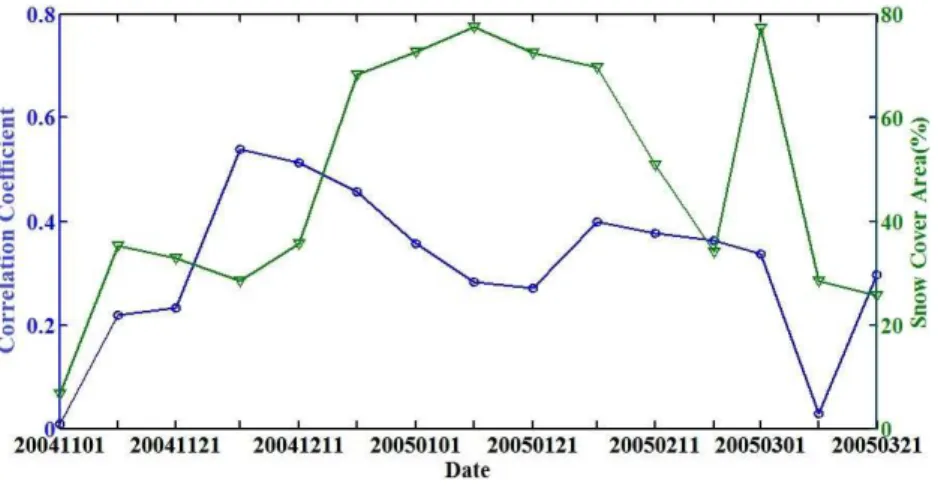
Figure 5 shows the evolution of the SCA and the correlation coefficient (R) between the snow depth and elevation in each 10 day period from 1 November 2004 to 31 March 2005. The varying trends betweenR and SCA during periods of the snow season are apparent.Rand SCA have similar increases at the beginning of the snow season.Rremains relatively stable (approximately 0.4) when the SCA exceeds 40 % 25

(11)

TCD

9, 4997–5020, 2015

C. L. Huang et al.

Title Page

Tables Figures

◭ ◮

Back Close

Full Screen / Esc

Discussion

P

a

per

|

Discussion

P

a

per

|

Discussion

P

a

per

|

Discussion

P

a

per

|

during the middle of the snow season. During the ablation period,Rdecreases sharply as SCA decreases.

Based on the observed snow depth at 46 meteorological stations, the MODIS-derived SCA, and the elevation, kriging methods are used to produce snow depth maps for each day. The cross-validation of the interpolated snow depth with the kriging 5

methods on the first day of each month is shown in Table 1. Comparing the adopted kriging methods (OK, UK, OCK, and UCK), the RMSE of OK is the smallest for 1 November and 1 December 2004. Less snow exists in the study area, and theR

between the snow depth and SCA is very small on these days. With increasing SCA and increasingRbetween the snow depth and SCA, the RMSE increases significantly; 10

thus, UCK achieves the best performance among the adopted kriging methods on 1 January, 1 February, and 1 March 2005. Thus, elevation is an important co-variable when most regions are covered by snow. Furthermore, the results using scheme-2 are more accurate than the results using scheme-1 in all cases. Adding virtual stations increases the number of samples and can thus somewhat reduce the interpolation 15

errors.

Figure 6 shows the spatial distribution of the estimated snow depth based on the best kriging method with the two schemes on 1 December 2004, 1 January 2005, 1 February 2005, and 1 March 2005. All maps predict deep snow in the northeast and southwest portions of the study area because of the mountainous terrain. Outside of 20

these areas, the maps estimated by the two schemes differ significantly. The maps of snow depth estimated by 2 are more detailed than those created by scheme-1. Additionally, the snow depths estimated with scheme-1 are much higher than those estimated with scheme-2, particularly in areas of deep snow. The scheme-2 spatial distribution of snow depth better matched the DEM and provided more detail. More 25

complicated and heterogeneous features of the snow depth distribution can also be seen in the results of scheme-2 because this scheme considers a greater number of virtual stations, thus increasing the number of samples.

(12)

TCD

9, 4997–5020, 2015

C. L. Huang et al.

Title Page

Tables Figures

◭ ◮

Back Close

Full Screen / Esc

Discussion

P

a

per

|

Discussion

P

a

per

|

Discussion

P

a

per

|

Discussion

P

a

per

|

4.3 Validation at independent meteorological observation sites

To assess the performance of the proposed scheme for snow depth interpolation, the observed and estimated snow depths at four independent meteorological stations are used. These data are shown in Fig. 7. The BIAS, RMSE, andRof the estimated snow depth at these four meteorological stations are listed in Table 2. The estimated snow 5

depth is computed by the optimal kriging method at each time step. Comparing these values to the measured snow depth at each station, the estimated snow depths with scheme-1 and scheme-2 capture the trend of the snow depth variation over the entire snow season (theR is greater than 0.89 for all stations), but the results produced with 2 are more similar to the observations than the results produced with scheme-10

1. The statistical indicators in Table 2 also suggest that the results of scheme-2 are more accurate than the results of scheme-1. The BIAS ranges from 2.84 to 5.80 cm for scheme-1 but only from 0.90 to 3.8 cm for scheme-2. The RMSE is reduced from 1.98 to 1.13 cm at the Fukang station, from 3.46 to 2.31 cm at the Beitashan station, from 2.65 to 1.37 cm at the Kelamayi station, and from 1.67 to 0.89 cm at the Tekesi station. 15

These results indicate that adding virtual stations without snow is useful for increasing the accuracy of the snow depth interpolation.

5 Conclusion and discussion

Blending visible satellite snow cover estimates to constrain the interpolation of snow depth/SWE is an useful way to improve accuracy of snow depth interpolation (Rice 20

et al., 2011). In this study, an optional interpolation scheme that produces a reasonable spatial distribution of daily snow depths using four types of kriging interpolation methods (OK, UK, OCK, and UCK) is proposed. The scheme combines the effects of elevation with MODIS SCA products. The daily snow depth observations at 50 meteorological stations in northern Xinjiang Province, China, are used to validate the 25

(13)

TCD

9, 4997–5020, 2015

C. L. Huang et al.

Title Page

Tables Figures

◭ ◮

Back Close

Full Screen / Esc

Discussion

P

a

per

|

Discussion

P

a

per

|

Discussion

P

a

per

|

Discussion

P

a

per

|

proposed scheme. The results suggest that the spatial distribution of the snow depth can be accurately reconstructed using the proposed method.

It is found that the elevation as co-variable is not always taken effect in the whole snow season. Early in the snow season, when relatively few regions are covered by snow, the correlation coefficient between the elevation and SCA is very low, and the OK 5

method produces the best snow depth estimation without using the elevation. Later in the snow season, when a large number of regions are covered by snow, the correlation coefficient between the elevation and SCA is relatively high; thus, the UCK method produces the best snow depth estimation. Therefore, the candidate kriging method should be dynamically determined each day according to the SCA conditions and the 10

correlation coe_fficient between the elevation and SCA.

Additionally, the accuracy of the interpolated snow depth is mainly determined by the number of the available stations. In this study area, only 50 snow depth measurements in each day can be used to generate the spatial distribution of the snow depth by the kriging method. Therefore, smoothing effects are always apparent in the results of the 15

estimated snow depths, particularly in mountainous regions where the snow depths are consistently overestimated. Adding a few virtual stations with zero snow depths, as indicated by the MODIS SCA data, can increase the number of observations and reduce the smoothing effect to yield more complicated and heterogeneous features in the snow depth distribution. The snow depth derived from passive microwave sensors 20

such as AMSR-E and SSM/I are also an important data source thought their spatial resolutions are very low. How to fuse all kinds of snow information (snow depth measurements from meteorological stations and derived from passive microwave sensors, and MODIS SCA products) to produce snow depth distribution with high-spatial resolution will be studied in next step.

25

Acknowledgements. This work is supported by the National Natural Science Foundation of China (grant numbers 91325106 and 41271358) and the Project of the One Hundred Person Project of the Chinese Academy of Sciences (grant number 29Y127D01).

(14)

TCD

9, 4997–5020, 2015

C. L. Huang et al.

Title Page

Tables Figures

◭ ◮

Back Close

Full Screen / Esc

Discussion

P

a

per

|

Discussion

P

a

per

|

Discussion

P

a

per

|

Discussion

P

a

per

|

References

Balk, B. and Elder, K.: Combining binary decision tree and geostatistical methods to estimate snow distribution in a mountain watershed, Water Resour. Res., 36, 13–26, 2000.

Birkeland, K. W., Hansen, K. J., and Brown, R. L.: The spatial variability of snow resistance on potential avalanche slopes, J. Glaciol., 41, 183–190, 1995.

5

Che, T., Li, X., Jin, R., Armstrong, R., and Zhang, T. J.: Snow depth derived from passive microwave remote-sensing data in China, Ann. Glaciol., 49, 145–154, 2008.

DeBeer, C. M. and Pomeroy, J. W.: Modelling snow melt and snow cover depletion in a small alpine cirque, Canadian Rocky Mountains, Hydrol. Process., 23, 2584–2599, 2009.

Elder, K., Dozier, J., and Michaelsen, J.: Snow accumulation and distribution in an alpine

10

watershed, Water Resour. Res., 27, 1541–1552, 1991.

Elder, K., Rosenthal, W., and Davis, R. E.: Estimating the spatial distribution of snow water equivalence in a montane watershed, Hydrol. Process., 12, 1793–1808, 1998.

Erxleben, J., Elder, K., and Davis, R.: Comparison of spatial interpolation methods for estimating snow distribution in the Colorado Rocky Mountains, Hydrol. Process., 16, 3627–

15

3649, 2002.

Goovaerts, P.: Geostatistics for Natural Resources Evaluation, Oxford University Press, Oxford, 1997.

Hardy, J. P., Davis, R. E., Jordan, R., Ni, W., and Woodcock, C. E.: Snow ablation modelling in a mature aspen stand of the boreal forest, Hydrol. Process., 12, 1763–1778, 1998.

20

Huang, X. D., Hao, X. H., Wang, W. et al.: Algorithms for cloud removal in MODIS Daily snow products, J. Glaciol. Geocryol., 34, 1118–1126, 2012 (in Chinese).

Jin, L., Ganopolski, A., Chen, F., Claussen, M., and Wang, H.: Impacts of snow and glaciers over Tibetan Plateau on Holocene climate change: sensitivity experiments with a coupled model of intermediate complexity, Geophys. Res. Lett., 32, 1–4, 2005.

25

Liang, T. G., Huang, X. D., Wu, C. X., Liu, X. Y., Li, W. L., Guo, Z. G., and Ren, J. Z.: An application of MODIS data to snow cover monitoring in a pastoral area: a case study in Northern Xinjiang, China, Remote Sens. Environ., 112, 1514–1526, 2008.

Marofi, S., Tabari, H., and Abyaneh, H. Z.: Predicting spatial distribution of snow water equivalent using multivariate non-linear regression and computational intelligence methods,

30

Water Res. Manage., 25, 1417–1435, 2011.

(15)

TCD

9, 4997–5020, 2015

C. L. Huang et al.

Title Page

Tables Figures

◭ ◮

Back Close

Full Screen / Esc

Discussion

P

a

per

|

Discussion

P

a

per

|

Discussion

P

a

per

|

Discussion

P

a

per

|

Molotch, N. P., Colee, M. T., Bales, R. C., and Dozier, J.: Estimating the spatial distribution of snow water equivalent in an alpine basin using binary regression tree models: the impact of digital elevation data and independent variable selection, Hydrol. Process., 19, 1459–1479, 2005.

Pebesma, E. J.: Multivariable geostatistics in S: the gstat package, Comput. Geosci., 30, 683–

5

691, 2004.

Pebesma, E. J. and Wesseling, C. G.: Gstat, a program for geostatistical modelling, prediction and simulation, Comput. Geosci., 24, 17–31, 1998

Pomeroy, J. W., Gray, D. M., Shook, K. R.,Toth, B., Essery, R. L. H, Pietroniro, A., and Hedstrom, N.: An evaluation of snow accumulation and ablation processes for land surface

10

modelling, Hydrol. Process., 12, 2339–2367, 1998.

Rice, R., Bales, R. C., Painter, T. H., and Dozier, J.: Snow water equivalent along elevation gradients in the Merced and Tuolumne River basins of the Sierra Nevada, Water Resour. Res., 47, W08515, doi:10.1029/2010wr009278, 2011.

Savelyev, S. A., Gordon, M., Hanesiak, J., Papakyriakou, T., and Taylor, P. A.: Blowing snow

15

studies in the Canadian Arctic Shelf Exchange Study, 2003–04, Hydrol. Process., 20, 817– 827, 2006.

Schmugge, T. J., Kustas, W. P., Ritchie, J. C., Jackson, T. J., and Rango, A.: Remote sensing in hydrology, Adv. Water Resour., 25, 1367–1385, 2002.

(16)

TCD

9, 4997–5020, 2015

C. L. Huang et al.

Title Page

Tables Figures

◭ ◮

Back Close

Full Screen / Esc

Discussion

P

a

per

|

Discussion

P

a

per

|

Discussion

P

a

per

|

Discussion

P

a

per

|

Table 1.Cross-validation of the snow depth spatial interpolation using various kriging methods.

Here, R is the correlation coefficient between the snow depth and elevation, scheme-1

represents the results at 46 meteorological stations, and scheme-2 represents the results at 46 meteorological stations and virtual stations.

Date SCA (%) R RMSE (cm) (scheme-1) RMSE (cm) (scheme-2)

OK UK OCK UCK OK UK OCK UCK

1 Nov 2004 6.701 0.001 0.292 0.297 0.296 0.338 0.226 0.235 0.228 0.232 1 Dec 2004 13.714 0.060 2.778 2.785 2.839 2.861 2.738 2.762 2.784 2.828 1 Jan 2005 72.626 0.347 9.974 9.071 9.912 7.842 6.601 6.413 6.045 5.984 1 Feb 2005 69.710 0.375 12.68 11.69 11.89 9.871 8.031 8.048 8.003 7.809 1 Mar 2005 77.352 0.338 12.12 11.12 11.84 10.33 9.917 10.33 9.894 9.477

(17)

TCD

9, 4997–5020, 2015

C. L. Huang et al.

Title Page

Tables Figures

◭ ◮

Back Close

Full Screen / Esc

Discussion

P

a

per

|

Discussion

P

a

per

|

Discussion

P

a

per

|

Discussion

P

a

per

|

Table 2.Bias and RMSE of the snow depth at four meteorological stations from November 2004 to March 2005. Here, scheme-1 represents the results at 46 meteorological stations, and scheme-2 represents the results at 46 meteorological stations and virtual stations.

Scheme-1 Scheme-2

Bias RMSE R Bias RMSE R

Fukang 3.329 1.981 0.941 2.132 1.126 0.963

Beitashan 5.801 3.464 0.950 3.794 2.316 0.964

Kelamayi 4.396 2.653 0.892 2.258 1.371 0.935

Tekesi 2.836 1.670 0.972 1.507 0.890 0.986

(18)

TCD

9, 4997–5020, 2015

C. L. Huang et al.

Title Page

Tables Figures

◭ ◮

Back Close

Full Screen / Esc

Discussion

P

a

per

|

Discussion

P

a

per

|

Discussion

P

a

per

|

Discussion

P

a

per

|

Figure 1.Distribution of meteorological stations in northern Xinjiang Province, China.

(19)

TCD

9, 4997–5020, 2015

C. L. Huang et al.

Title Page

Tables Figures

◭ ◮

Back Close

Full Screen / Esc

Discussion

P

a

per

|

Discussion

P

a

per

|

Discussion

P

a

per

|

Discussion

P

a

per

|

Figure 2.Spatial interpolation scheme for snow depth with kriging methods using ground-based snow depth observations, MODIS snow cover areas, and elevation.

(20)

TCD

9, 4997–5020, 2015

C. L. Huang et al.

Title Page

Tables Figures

◭ ◮

Back Close

Full Screen / Esc

Discussion

P

a

per

|

Discussion

P

a

per

|

Discussion

P

a

per

|

Discussion

P

a

per

|

Figure 3. Time series of snow-covered pixels among MOD10A1, MYD10A1, and cloud-removed MODIS snow cover area products from November 2004 to March 2005.

(21)

TCD

9, 4997–5020, 2015

C. L. Huang et al.

Title Page

Tables Figures

◭ ◮

Back Close

Full Screen / Esc

Discussion

P

a

per

|

Discussion

P

a

per

|

Discussion

P

a

per

|

Discussion

P

a

per

|

Figure 4.Maps of snow cover areas on 1 December 2004 (left column) and 1 February 2005 (right column), derived from (a1andb1) MOD10A1, (a2andb2) MD10A1, and (a3andb3) the cloud-removed images.

(22)

TCD

9, 4997–5020, 2015

C. L. Huang et al.

Title Page

Tables Figures

◭ ◮

Back Close

Full Screen / Esc

Discussion

P

a

per

|

Discussion

P

a

per

|

Discussion

P

a

per

|

Discussion

P

a

per

|

Figure 5.Evolution of the snow cover area and the correlation coefficient between the snow depth and elevation in northern Xinjiang from 1 November 2004 to 1 March 2005.

(23)

TCD

9, 4997–5020, 2015

C. L. Huang et al.

Title Page

Tables Figures

◭ ◮

Back Close

Full Screen / Esc

Discussion

P

a

per

|

Discussion

P

a

per

|

Discussion

P

a

per

|

Discussion

P

a

per

|

Figure 6. Spatial distribution of the estimated snow depth on 1 December 2004 (first row), 1 January 2005 (second row), 1 February 2005 (third row), and 1 March 2005 (fourth row). Scheme-1 (left column) shows the interpolation results at 46 meteorological stations, and scheme-2 (right column) shows the results at 46 meteorological stations and virtual stations.

(24)