Relative price dynamics, factor shares and endogenous growth

(1)

UNIVERSIDADE TÉCNICA DE LISBOA INSTITUTO SUPERIOR DE ECONOMIA E GESTÃO

Masters: Economics

RELATIVE PRICE DYNAMICS, FACTOR SHARES AND ENDOGENOUS GROWTH

ARMANDO DOS SANTOS RIBEIRO FERREIRA

Supervisor: Prof. Doutor Paulo Meneses Brasil de Brito

Assessment Committee;

Chair examiner: Prof. Doutor Paulo Meneses Brasil de Brito

Other Examiners; Prof. Doutora Maria Isabel Sanchez Horta Correia Rio de Carvalho Prof. Doutor Luis Filipe Pereira da Costa

(2)

Relative Price Dynamics, Factor Shares and Endogenous Growth Armando dos Santos Ribeiro Ferreira

Masters: Economics

Supervisor: Prof. Paulo Meneses Brasil de Brito Approved on:

Abstract

We present a two sector general-equilibrium model of endogenous growth for a small open economy. We show that the model lias saddle-path stability independently of the factor intensities, however the details of the transitional dynamics will diífer. The dimension of the stable manifold is always one but the slope of the stable manifold changes depending on the factor shares. If the factor shares are such that each sector uses more intensively its own capital, then after a shock the economy will adjust through prices variations. When the factor shares intensities are reversed, the adjustment is made through quantities variations. Moreover we find that a productivity shock on the traded sector has always a positive effect on the relative price. Government demand shocks have no long run effect on the relative price and its effect ou the GDP is not clear.

Keywords: Real exchange rate, Non-tradables, Relative price, Endogenous growth

JEL Classiíication: F43, 041

Resumo

Modelizamos uma pequena economia aberta cora dois sectores e crescimento endógeno. Mostramos que o modelo apresenta estabilidade tipo sela inde- pendentemente das intensidades factoriais, no entanto as propriedades da dinâmica de transição vão diferir. A dimensão das trajectórias convergentes é sempre um mas a inclinação muda dependendo das proporções dos fac- tores. No caso de cada sector usar mais intensivamente o seu próprio capital, após um choque, a economia vai estabilizar por variações nos preços e no caso contrário a estabilização é feita por variações nas quantidades. Alem disso, mostramos que um choque de produtividade no sector transaccionável tem sempre um efeito positivo no preço relativo. Choques governamentais de procura não têm efeito de longo prazo no preço relativo e o seu efeito no produto não é claxo.

(3)

Index Abstract Table of Tables .. Table of Figures . Acknowledgments 1. Introduction 2. The model 2.1. The GDP function ... 2.2. Consumption 2.3. Intertemporal problem 8 2.3.1. General-equilibrium 9 2.3.2. Balanced growth path 9 2.4. Transitional dynamics 12 2.5. Multipliers 16 2.5.1. Case 1: det{B) >0 18 2.5.2. Case 2: det{B) <0 19 3. Application 21 3.1. Government demand shocks 21 3.1.1. Case 1; dei{B) >0 22 3.1.2. Case 2: det{B) <0 23 3.2, Productivity shocks 24 3.2.1. Case 1: det{B) >0 24 3.2.2. Case 2: dei{B) <0 25 4. Numerical illustration 27 ii

(4)

4.1. Parameter values 27 4.2. Government deinand shocks 28 4.2.1. Case 1: det{B) >0 28 4.2.2. Case 2; det{B) <0 31 4.3. Productivity shocks 34 5. Conclusions 37 References 40 Appendix 41 iii

(5)

Table of Tables

Table 1 : Slope of the stable manifold if det(£?)> 0 15 Table 2 : Base Line parameters 28

(6)

Table of Figures

Figure 1 : Demand shocks for det(£J)> 0 29 Figure 2 : Demand shocks for det(fí)< 0 32 Figure 3 : Productivity shocks 34

v

(7)

Acknowledgments

Writing this dissertatiou was truly a challenge, not only because of the efFort required but also for the psychological and physical absence my friends and family had to endure.

I specially want to thank Prof. Paulo Brito for having accepted to be my supervisor, for guiding me towards an extremely interesting subject, for help- ing me when I needed, for the words of incentive that he gave me (sometimes even unknowingly) but mainly for the patience and for the friendship that he revealed throughout the whole process. Without him I surely could not have accomplished this dissertation.

I am also very grateful to Prof. Luis Costa, for believing in me from the very beginning of my undergraduate studies in economics. Without his ad- vice I most probably would never have chosen to take the masters degree in economics.

To Sofia Loureiro I am grateful, among other things, for having provided the computer that was used to write this dissertation.

My gratitude goes also to Victor Lima for the important friendship that we have, for the many times that he read my dissertation and for the helpful revising and comments.

Finally I reserve my deepest gratitude to my parents and brother, for having helped in so many different and important ways.

(8)

Chapter 1

Introduction

This dissertation presents a two sector model of endogenous growth for a small open economy with both tradable and non-tradable capital which are used in investment and production. We assume that the economy is a price taker for the traded good and the law of one price holds for this sector which is consistent with Gregorio et al. (1994) in particular for the euro area. The non-traded sector is not subject to international competition so the price is set in autarky.

Due to the properties of the production functions we have a unique balanced growth path (BGP) for the economy that works as a trend for the variables. Through a detrended system, we study the dynamics of the deviations from the balanced growth path caused by a shock.

Having in mind that the relative price of non-traded goods can be a good proxy for the real exchange rate, the main objective of this dissertation is to understand the dynamics of the relative price of non-traded goods, how it affects the economy and how can policy rnakers use it to improve the perfor- mance of a small open economy. Moreover, we intend to develop an easier and more clear approach to understand the transitional dynamics of such a model.

There are several papers in the literature dealing with the dynamics of two sector models (mainly the dynamics of the Uzawa-Lucas model) however they study closed economy models. Examples of these papers are Romer (1986), Rebelo (1991) and more recently, Mulligan and Sala-I-Martin (1993), that use numerical methods to lind saddle-path stability for the Uzawa-Lucas model. Bond et al. (1996) have a similar approach to ours and also íind saddle-path stability independently of the sectoral intensities. Although the dimension

(9)

//A. /

of lhe stable manifold does not change when lhe relative intensities changes (like ours), lhe slope of lhe stable manifold remain lhe same (which is a different result from ours).

The number of papers thal study these issues for open economy models is much smaller (see Turnovsky (2002) for a survey). Turnovsky (1996) presents the same model as ours however but solves it using a completely different strategy. He does not consider the existence of a comraon balanced growth path, therefore the model is not stationary. He studies the local dynamics only for the relative price and the price of installed traded capital. He concludes that if each sector is intensive in its own capital then they have saddle-path stability type and total instability if the factor intensities are reversed, in particulary, the dimension of the stable manifold differs depending on technology of the factor shares. Meng (2003) presents Turnovskys model with externalities and follows the same strategy to solve it.

Our strategy will be quite different. We first solve the intra-temporal allo cations of the capital stocks between sectors. Then we do the same for the static decision between the consumption of traded and non-traded goods. Af- ter having solved the intra-temporal problem, we focus on the inter-temporal problem applying to Pontriyagin maximum principie. We construct the 6x6 Jacobian and applying to Moore-Penrose method we can íind long and short run multipliers for demand and productivity shocks.

Although we only changed the strategy to solve the model, the results are very different. The most important finding is that the dimension of the stable manifold is one and does not change when the factor intensities change, however the slope of the stable manifold does. Another interesting result is that, after a shock the economy will adjust through prices if each sector is relatively more intensive in its own capital and through quantities when the relative intensities are reverse. Furthermore we íind that au increase in government consumption of traded good will have a positive effect on the GDP independently of the sign of the factor shares, and an increase on public consumption of non-traded good will have the opposite effect. To what concern the relative prices, demand policies are neutral on the long run. Finally we show that a productivity shock on the traded sector has long run effects both on the relative prices, capital stocks and externai debt.

The dissertation is organized as follows. In the next section we develop and solve the model. In section 3 we study the policy variables by performing demand and productivity shocks. In section 4 we calibrate the model and present a numerical analysis and in section 5 we explain our conclusions.

2

(10)

Chapter 2

The Model

We assume that this is a small open economy inhabited by an infinitely lived representative agent and where the population is constant. The agent accumulates two types of capital, tradable (A't(r)) and non-tradable (A'n(r))

which are used as inputs in the production of traded output (^(r)) and non-traded output (V^r)). r is the time index. The traded and non-traded capital depreciation rates are ôt and õn respectively and are assumed to be

positive. He also accumulates foreign bonds, jB(r), that pay an exogenously given world interest rate, r. The government collects a lump-sum tax,7', consumes traded and non-traded goods Gt and Gn respectively and the gov-

ernment budget is always in balance, that is , T(r) — Pí(T)Gt + P„(r)Gn

where P((r) and P„(t) are the nominal prices of the traded and non-traded goods respectively.

We denominate Kj, j = t,n as being j capital used as input at traded good production. The same applies for K™, j = t,n which is the j capital employed in the non-traded sector production. The rates of capital accumulation for traded and non-traded sector respectively are denoted by ^(r) and /«(r) and the consumption of traded goods by Gf(T) and non-traded goods by

Gn(T). The initial values for the capital stocks and foreign bonds are given,

Art(0) = At0, A'n(0) = A^, P(0) = Bo, and p is the time discount rate.

Moreover, the accumulation of traded capital is subject to convex adjustment costs, ( and the equilibrium condition (Tn(r) = Gn(r) + /«(t) + Gn)

is verified for the non-traded sector. The agent chooses the paths for G^r), G„(r), hir), /n(r) and for the capital allocations A'tt(r), K^t), ^"(r), A^(r)

in order to solve his optimization problem.

(11)

Z"00 6Xr)1_<T - 1 _ot , / e p a,/9>0 Jo l — a max subject to C{t) = [Ct{T)]e [Cnir)]1-9 Ktir) = It{T) - ôtKt{r) Knir) = Ur) - 6nKn{r) Yt{T) = A, [^(r)]^ [^(r)]'"^ Yn{r) = AnWiT)]1-^ [KZ{r)f" Kt{T) = KI{T) + K?{T) Kn[r) = K^{t) + K£(t) Pt(T)B(r) = Pt(T)Yt(T) + Pn(T)Yn(T) ~ Pt(r)Ct(T) - Pn(T)Cn(r) - Pt(T)ft(T) (l + - Pn{r)Inir) - Pf(r)T(T) + ri3(r)

We will solve the model in three separate parts. First we find the intra- temporal allocations of both capital stocks. In the second phase we will solve the static program for the decision between consumption of tradable or non-tradable goods. In the last phase we use the static conditions found in step one and two and solve the intertemporal model where the agent chooscs the levei of aggregate consumption, and the levei of investment in traded and non-traded capital.

2.1 The GDP Function We define the GDP function by1:

g = max{PtYt + PnYn : given Yt and /„} (1)

The matrix of technological coeflicients can be written as: B:= Pt i - A

1 - A» Pn (2)

'This methodology is used by Brito and Pereira (2002b) for two sector models and by Brito and Pereira (2002a) for three sector models.

(12)

Note that the relation det(fí)-tr(5) + l=0 holds. Thus, if the sectors are relatively more intensive in their own capital then tr(/5)-l> 0 we have det(1B)> 0.

If the intensities are reverse then tr(fí)-l< 0 and therefore det(1B)< O2

The Lagrangian function for the above problem (1) is given by:

£ - PtYt + PnYn + RtiKt - Kl - K?) + fín{Kn -K^- K^) (3)

Where Rt and Rn are the Lagragian multipliers.

Solving the maximization problem (3) we obtain the GDP function Ç. Q = PtYt + PnYN = R,Kt + RnKn

The outputs from the traded and the non-traded sectors are given by the Rybczynski functions.

y> = + (4)

y- = ~=^Kt + 4,a^Kn (5)

(Ji n rn rn

where ipu, i, l = 1,2 are the elements of and Rj j = t, n are the nominal rates of return for asset Kj which are given by the Stolper-Samuelson equations:

H. = ~ = (6)

Rn = ~~ = (P, A,/};)*''(PnAnK)**' (7)

for p* = ${1 - Pj){x~^\ j = t,n.

If we represent the GDP function in terms of the traded good as, F = p-, then (4) and (5) can be written as:

Yt — dttKt + 0,tnKn (8)

Yn — o-ntKf T (inn Kn (9) 2For more detaíls on the properties of the B matrix, soe Brito and Pereira (20()2a).

(13)

where: Pn att - teW)rt 1 Pn a,n ~ det{B)prn - 1 ~ Pt ri 0ní det{B) p Pt det{B) n

and p = -^ is the relative price. Note that att, am, o-nt, ann are functions of

the B determinant.

Dividing equations (6) and (7) by the price of the own sector, such as, r, — we have the real rates of return which are also function of det(B) and are given by: rt = nit (10) rn = mnp^u (11) Where; = (A. /?)*" mn = (At 01)*" (K 0')*"

This is linked with the Rybczinsky and the Stolper-Samuelson theorems. As we saw previously, if det(Z?)> 0 which implies that att,ann > 0;aín,an( < 0,

then an increase in the own capital will increase the optimal levei of output in that sector and reduce the production in the other sector. If we have the opposite sign for the det(fí) then an increase in the own capital will reduce the production in own sector an rise it on the other sector. The same applies to Stolper-Samuelson theorem. If the sector is intensive in its own capital, det(jB)> 0, an increase in the relative price, p, will reduce the real reward of the factor used intensively (in this case traded capital) and increase the real reward of the other factor. If det(R)< 0 the relative intensities are the opposite, an increase in p will reduce the real reward of traded capital and increase the real reward of non-traded capital.

(14)

2.2 Consumption Composition

The agent chooses the amount of consumption of each good in order to minimize his expenditure subject to a certain levei of utility, that is:

E{Pu Pn, C) = min {PtCt + PnCn ■. v<C], (12)

Ct,Gn

Using the intratemporal sub-utility function of Turnovsky (1996), we can build the Lagrangian function for the problem:

c = PtCt - PnCn + Qc{C - (Ct)0 (O,)1-*)

Solving the above maximization problem, we obtain the Hicksian demand functions i. e. the optimal static allocations for consumption of each good.

c. = (13)

õ. = c(^)' (14)

Total expenditure is given by:

Ê{PuPn,C) = P?PtdCw{0) (15)

Where zu{0) — O~0{1 — O)9'1.

Dividing (15) by the price of tradables goods, we can write total real expenditure as a function of C and p;

è(p, C) = rn^Ç) = (18)

where w{Q)px~6 is the reciprocai of the real exchange rate 3.

3With the chosen utility function, the real cost of living índex is given by pl~etz{e).

Assuming the nominal exchange rate equal to one (as in the Euro arca), we find the real exchange rate R = (c7($)pl~<')~1- As one can see, the exchange rate has a monotonic

relation with the relative price.

(15)

2.3 Intertemporal Problem

Once that we have already solve the intra-temporal problem, we can now solve the intertemporal problem, where the agent choose its levei of aggregate consumption, investment in both sectors, anel the leveis of the capital stocks. The solution for the problem can be obtained by maximizing the current value Hamiltonian.

H = C^1 a - 1 + Qtihir) - StKt{T)) + Qn{In{r) - Ín/Cn(r))+

1 — cr

+Qt(Y(T) - e(p, C, t) - It(r)(l + ^- p(r)/„(r) - +

The optimal instantaneous leveis for consumption and investment are determined from the íirst order conditions

c = [QbVl-de-9{i-e)-^-6)]~l (i?)

I = i+l (i8)

Qn = QbP (19) Where Qt, Qn and Qb are the instantaneous values for the co-state variables associated with the stock of traded capital, non-traded capital and externai net asset position.

Note that adjustment costs for the traded sector are essential to avoid indeterminacy in the optimal rate of traded capital accumulation lt. We do not

consider the existence of adjustment costs in non-traded sector because we would lose the simple way to endogenise p that is give by equation (19). If we consider adjustment costs in the non-traded sector, the equality p — ^

(equation (19))is lost therefore we need to íind an alternative way to make p endogenous. This is possible, however the model becomes to complicate 4

Pontriyagin maximum principal give us the dynamic system;

Qb = Qb{p-r) (20)

/ o (ÇÍ-1)2 (nu

Qt = Qt{r + ôt) -n (21)

4The other papers in the literature also consider adjustment costs for traded sector

only. See Turnovsky (1996) and Meng (2003). 8

(16)

P = p{r + ón- rn) (22)

(23)

Kn — In 6nKn (24)

(25)

lim BQhe pt = 0; lim qtQbKte pt = 0; lim QbpKne pt = 0

í—too t—too Í-+00 2.3.1 General-Equilibrium

Using the equilibrium equation for the non-traded sector (/„ = Yn — Cn — Gn)

and assuming that the government budget is always in balance (T — Gt + pGn), we can write the model as;

The general-equilibrium is represented by equations (26)-(31), plus initial and transversality conditions.

2.3.2 Balanced Growth Path

Let X be a generic variable with a trend and let the corresponding detrended variable be denoted by x. Then X = x exp(7xí) where 7X is the long run

growth rate of X and x are the deviations from the long run growth path.

Qb = Qbip-r) (26) (27) (28) (29) (30) (31) , . c \ (ft-l)2 Qt = qt(r + 6t)-rt —— P = p(r + ôn - rn) Kn — h i "1 (jlnn &n) Kn Gn 9

(17)

Using this deíinition 5, and having in mind that along the balance growth

path we have 7fet = 7fcn = 76 = Igt = Ign = "Igh/v = 7 and %t = lv = 0, we

can write the system in detrended variables as:

<76 = <76(p ~ r + 0-7) (32) qt = <7Í(^ + àt) -U- ^ (33) p = p (r + - rn) (34) k = (35) ^ Untkt (^nn T) 9n (^®) h = faít + ^2^ ~) + aínfcn " ^ ~ ft + (r - 7)b (37)

Where pf and gn is the weight of public expenditure on GDP.

The transversality conditions become:

lim bqbe-{p+^-l))t = lim qtqbkte-^a-l))t = lim pq^e'^^-1^ = 0

t—>oo í—>00 t--»oo We obtain the long run growth rate from equation (32)

7 = ^ (38) cr

The steady state for the relative prices is given by equation (34) after substituting rn 6 det(B) 1 —0n (39) V + sn \ rrin ] From equation (35) we obtain:

çt = l + ^t + 7) (40)

which should also be the equilibrium point for equation (33). This will only be true for a particular choice of parameters, namely:

1 —&t.

m,(r-^)" =tlt(r + St)~l{Sl+rf (41)

\ TTín ) ^

5This definition is from Brito and Pereira (2002a). 6 Note that ipn = ^y.

10

(18)

The parameter An is set to A*n to guarantee that (41) holds, that is: An — An — Af (r + Sn V ^ . r + ôt + jrjSt + 7) + - 72) 1 "Pn 1 - Bt (42)

Note that the way we calculate qt is complctely different from Turnovsky

(1996) and Meng (2003). They calculate it through equation (33), then substituto it on (35) and use the result as the long run growth rate of traded capital, so, they obtain a completely unstable rnodel.

Finally kn and qb are given by equations (36) and (37) respectively and verify

the two dimensional manifold:

kn Qb = <tkt - CniQbiP) - 9n ^ + 7 - <n i-W-t) / n \ 0-1 P " ( V \ (43) zo{6) i-e. att + t 2^ - ) A: t + a*tnkn - gt + {r- 7)6 (44)

where the * means that An is already substituted by A*.

Proposition 1 (Existence of a BGP)

A balance growth path, as we dcfined prévio tis, exits if and only if • r > p > r(l — a)

l~f>n

= A" ('it) r+ôi+ír((5t+7)+ Í(Sf —p)

These conditions are also necessary for the existence of a steady-state point for the detrended dynamic system.

Proof: The íirst point of proposition one guaranties that we have positive growth and that the transversality conditions hold.

1. r > p implies that 7 = 7^ > 0

2. p > r(l — a) implies that p + 7(0" — 1) > 0 and so the transversality conditions are veriíied.

11

(19)

The second point of proposition one guaranties that the arbitrage conditions are veriíied. /l* is calculated in order to solve the following conditions:

? + = r+ít

Qt 2Çqt

rn = r + ô. 71

Note that the necessity to tie A*n is due to the fact that we have three equa-

tions to solve (33), (34), (35) and only two variables to solve them p and qt. ■

2.4 Transitional Dynamics

By analyzing the dynamic system we can see that the explicit solution is not possible because p enters in nonlinear form in equation (33), thus we will study the approximate local dynamics in the neighborhood of the BGP. The variational system is represented by the six dimensional system of ordinary differential equations x{t) — Jcdx(r) + S(Íj(t), where Jc is the Jacobian

evaluated at the steady state, x = [qb,qt,P, h, km b]' and z = [gt, yn, At,]'.

For the time being we focus just on x{t) — Jccíx(r). The Jacobian, evaluated

at the BGP leveis is: 0 0 0 o cn aib _Ç£_ ^96 0 r — 7 0 it í 0 qÃt ( Çn. a o Qnt P 0 Í53 - PJ53 0 0 0 0 ^nt O-tt + 9?-2 _2Í 0 0 0 0 r — 7 — (Itn atn P 0 0 0 o o r — 7 (45) Where; J53 — da., nt dp ki + dcLnn t- dp kri dCn dp

Ct and Cn can be found using equations (13) and (14) respectively, together with equations (17) and (44).

Next we determine the eigenvalues of the matrix Jc

12

(20)

Lemma 1 Eigenvalues

The eigenvalues of the Jacobian are given by

Ai,2 = O (46) As,6 = X > O (47) \ (1 —/?n)(^ + An) A3 - " dem (48) = (Jtr + (1 - ÃOjn _ 4 det{B) 7 [ '

Proof: Applying to Brito (1999), we write the characteristic polynomial as:

c{Jc,A) = ^(-l)iM6_iAi (50)

i=0

Where Mi is the sum of the principal minors of order í — 0... 6 and we use the convention M0 — 1.

Considering the relations between the elements of the Jacobian (see annex), we can rewrite the characteristic polynomial as:

C(A) = A2(A-x)2(A-^)(A-X+V) (51)

/ Jr Where:

x = r_7

From equation (51) we can directly calculate the eigenvalues which are given by: 1,2 = 0 \ atn A3 — p A4 = X- '5,6 = X det{B) O-tn 4" (1 fln)dn p det{B) -7

which are the values of (46), (47), (48) and (49). ■

Assuming that the transversality conditions holds, then r - 7 > 0. In this 13

(21)

case we have two zero eigenvalues and another two that are equal to r — 7 and therefore positive. The sign of the other two eigenvalues, depends on the factor intensities. If det{B) > 0, then it is easy to see that A3 < 0 and A4 > 0. If we have the reverse intensities, such that det{B) < 0, then the signs of these eigenvalues also change becoming A3 > 0 and A4 < 0. The signs of the eigenvalues can be summarized by the following proposition: Proposition 2 Assuming that the transversality conditions and the conditions for the existence of a BGP are venfied. Then:

1. Ifdet{B) > 0, then we mil have two null eigenvalues (46), three positive (47) and (49) and one negative given by (48).

2. lfdet{B) < 0, then we will have two null eigenvahes (46), three positive (47) and (48) and one negative given by (49).

From proposition two, it is clear that the we have saddle-path type stability independent of the relative intensities, so the dimension of the stable manifold is always one. Note, however that the stable eigenvalue, i.e. the negative one, changes when the relative intensities change. Our result is different from the one of Turnovsky (1996) and Meng (2003). They have different types of stability and the dimension of the stable manifold changes with the relative intensities. If the traded sector is intensive in its own capital, then the stable manifold is of dimension one. They have saddle path stability for the relative price. If the traded sector is intensive in non-traded capital, then the stable manifold has dimension zero, so the dynamics for relative price is completely unstable. As we said prcvious Turnovsky (1996) and Meng (2003) don't have a stationary equilibrium for the complete model, they analyze only the sub system [qt p]', being the results for the dynamics only for the subsystem. Lemma 2 Eigenvectors

The matrix of the eigenvectors of the Jacobian is:

P=[P1 F2 P3 Pu P5 P6 ] (52)

• If det{B) > 0 then s=3 and u=4 • If det{B) < 0 then s=4 and u—S

14

(22)

where Pz, z = 1... 6, is the eigenvector associated to the eigenvalue i 7.

As we saw previous, the stable eigenvalue changes when the relative intensities change. Being so, the slope of the stable manifold is also different depending on the factor intensities, i. e. on the sign of det{B). The third collum of the P matrix switch with the fourth collum.

Proposition 3 Slope of the stable manifold

1. If det{B) > 0 then the slope of the stable manifold is: p* = P*=\O,PIPÍ,P!,P*,I]'

The signs of P* can be quite different depending on the parameter values. In particular there are two criticai values for ^53 which are the points where the signs change. The possible signs are describe in tablel8

Table 1: Slope of the Stable Manifold if det{B) > 0 0 < J5.3 < Í53c J53 = Í53c J53c < J53 < Í53d J53 > jss., pS + + + - - - - + P! - - - + pí - 0 + - Where: js'ic = ktidntpf (.(it7l\pir - 7) - atn] - p[(r ~ 7)(atnCcn + pdntktcrqt) - ÍP(ínt)2kt(T - - 2a?n£cn •753d " P<y&tn\p{r - l) ~ atn]

j53c and j53rf are both positive.

2. If det{B) < 0 then the slope of the stable manifold is: P* = P* = 0,0,0,0,—z,l

P Where it is clear that P5 — —p < 0

7See demonstratiou 1 in the appendix for mores details on the eigenvectors matrix. 8See demonstratiou 1.

15

(23)

The existence of two zero eigenvalues is know in this type of models, one is due to the fact that we are studying an endogenous growth model and the other is because we have assumed the economy to be small. The negative eigenvalue is generated by the existence of a second sector of consumption goods. This is a new result, in the literature these type of models tend to be explosive, that is, there are only the zero eigenvalues and the positive one. Another interesting result of the model, is that when the sectors are relatively intensive in its own capital there is a price adjustment and when the factor intensities are reversed there is a quantity adjustment. As you notice, the negative eigenvalue change depending on the sign of the When we have det(fí)> 0 the negative eigenvalue is A3, so the economy adjustment is made through variations on the relative price. In the case of negative B determinant, the negative eigenvalues is A4 therefore the economy adjusts through Kn quantities variations.

2.5 Multipliers

Recalling the variational system: 9

x(r) = Jcdx(r) + Sdz^r)

In order to íind the solution for the variational system, we define 10

N(r) = x(r) - x (53) x is obtain from the variational system. Knowing that det(Jc) — 0, it can be

proved that:

x = -J+S + (/ - Jc+Jc)k (54)

Where k = [/«i, «2, «3, «4, «5, «e]' 's a vector of constants and Jcf = PJjlP-1

is a generalize inverse of the Jacobian (45). is a generalize inverse of the Jordan's matrix associated with the Jacobian (45). As you notice, we need to calculate Jordan' s matrix in order to find Jj". This is quite simple because we have already calculatcd the eigenvectors matrix. Jordan form associated with the Jacobian is given by Jr = P_1JoP and veriíies the condition PJr =

9See Mulligan and SalaTMartin (1993) for a closed economy version. 10See Brito (2003) for a more detailed explanation about this method.

16

(24)

JCP. Jordan form is a diagonal matrix with the eigenvalues on the principal

diagonal11 , so, its inverse is:

P^JJP = 0 0 A 0 0 0 0 0 0 0 0 0 0 0 0 0 0 0 0 A4 0 0 0 _A51 0 0 0 J_ _{As .} (55)

Next we make the transformation

u{t) — P"_1A^(í) —> ú{t) — Jru;(í)

where P is the matrix of the eigenvectors (52), and Jr is Jordan's matrix.

The solution for this system of equations is

w(r) eJrth (56)

Where e^rt is the exponential matrix for Jr and h is a vector of constants.

We eliminate the explosive part by setting /14, h5 and hç to zero, thus the

solution, (56) is:

cJi(r) = hi = h2 Uz{T) = hsex'T

cJ4(r) = lõ5{t) = cJ6(r) - 0

Now we can make the inverse transformation: N(r) — Puj(r)

Using this result on (53), the solution for the variational system is given by: x(r) = x + N(t)

After substituting N(r) in the above expression, we obtain the approximate values of the variables in the neighborhood of the BGP

x(r) = x + P1/'-! + P2h2 + Ps/i3e A., 7 (57) uSee demonstration 2 011 the appendix.

17

(25)

Where x = x + P /ii + P2/i2 are the long run niultipliers 12 , A., is the

negative eigenvalue, P''í is the eigenvector associated with it and hi, h-i and

/13 are constants to be determined 13.

Let Sa, í = 1... 6 be elements of the vector S associated with a generic shock, and let , í = 4 ... 6, £ = 1... 6 be the elements of (/ — Jch Jc), then (54) is

given by: Qb Qt P k kn b «1 M21 ^31 ^41 + Z)?=2 finKe + «4 ^51 + 12e=i (heK( Atei + Tj=i (58)

where: fitj is the element of the vector - J^S = [/^]íj=i,.,.,6 14-

Once that the slope of the stable manifold depends 011 the sign of det{B), we will consider the two cases separately.

2.5.1 Case 1: det(Í?)>0

If the factor shares are such that {det{B) >0) then the negative eigenvalue is A3, therefore the associated eigenvector is P3. The paths for the variables

after a generic shock are given by the following system. <]b{r) = QÁr) = Qb Qt P?beX37 Where: Qt p{r) - V-Pfhe^ kt(T) - P43(l-eA^)ò kn{r) = P53(l-eA3T)5 6(r) = (l-eA3T)ò antdet{B) r — 7 -S21 + (r-7)(l-/3n)r, ■S31 (59) (60) (61) (62) (63) (64) (65)

,2Note that x are also the steady-sate values for the detrended system as defined above 13See Demonstration 4 and 5 for more details on how to find the values for hi, /12 and

hs.

14See demonstration 3 on the appendix for more details 011 the //, vector.

(26)

(68) (67)

and

D' = Pl + PlPl - P43

From the above system we can see that the only variable that is not subject to transitional dynamics is qb which jumps immediately to its new steady state value. On ali other variables, a shock has both long run and transitional effects. Both capital stocks and externai debt will deviate from the balance growth path and return to it on the long run 15.

By analyzing the long run value for the relative prices, p, we can see that its sign is function of the factor shares. Furthermore we find that a shock only has long run effects on relative prices if it affects S31.

In this case, the stable eigenvalue is A4 and the associated eigenvector is now

P4. The paths for the variables after a shock are now given by 16:

2.5.2 Case 2: det(^)<0 flb{T) Qt{r) p(t) h{r) Mt) 6(r) Qb Qt P 0 P4(l-e^)ò (1-6^)5 (69) (70) (71) (72) (73) (74) Where: 1 621 (r-7)(l -/?n)prn531 (1 - Pt)rt Qt _{r - 7}

15See demonstration 4 for more details 011 the system (59)... (64). 16See demonstration 5.

(27)

P — 7^ TTx—«31 (1 ftnyn 5» = ^|-(íí + ff ísl/Wi + (Plpi - P ~ (P,'P!PÍ-P?PjPÍ)v<ii! and D" = Pi + P42P54

Several interpretations can be made over the system (69) ... (74): First we see that there is no transitional dynamics for the price of installed traded capital nor for the relative price , after a shock they both jump immediately to their new steady state value. The second interesting result is that no shock can affect the accumulation of traded capital which evolves always along the balanced growth path with out deviations. Finally, after a shock, both the stock of non-traded capital and the externai debt, start form an initial point and have transitional dynamics until reach their new steady state levei.

(28)

Chapter 3

Applications

In this section we analyze the qualitative effects of government dexnand shocks and productivity shocks. The S matrix can be seen as a policy matrix, in the sense that although we choose just three variables to perform shocks on the economy, many others can be easily added.

To find the qualitative effect of each shock, we use the collum of the S matrix associated with that shock. Each shock will imply a different value for the elements of S, 5^, í = 1,..., 6 and therefore different long run effects. After calculating the S vector, we use the expressions of /qi, í = 2,..., 6 on the dynamic system and obtain the paths for the variables.

3.1 Government demand shocks

We start by analyzing the effects of fiscal policy. If the government increases its consumption on the traded good, gt, the elements of the S vector are ali zero except Sgi = — 1.

If the increase is on non-tradcd good we have ali elements of the S vector equal to zero except S51 = — 1-

Substituting these values on the generic /x vector, we obtain:

//21 = 0 (75) fkn — 0 (76) AMi = 0 //51 = ^ (77) (78) 21

(29)

//61 — (í.(i) — 1)- h i{i) .^65

J22 J55J22 (79)

where t{i) — i — l and i takes value one when the goverument increases its consumption on the traded good and two when the shock is over the non- traded good. ^22, jsn, ies are elements of the Jacobian k

Given the importance of the sign that the determinant of the B matrix has for the dynamics, we have to study the two cases separately.

3.1.1 Case 1: det(i3)>0

Substituting (75)... (79) on the system (59) ... (64) we obtain the approximate paths for the variables after the shock.

Qbir) = Qbg (80) Qtir) = -P2369eA3r (81) P(t) = -PfbaeXar (82) fct(r) = P^{1 — eX3T)bg (83) kn{T) = P3 (1 — eX3T)bg (84) 6(r) = (l-eA3r)59 (85) ba - (]bQ where: J_ -det{B)p{i{i)ct + (t(z) - l)c,t) D' rt{ct + põr^iPt - 1) - CnfQtdetíB)^ - 7)_ ÍKP/PÍ - Pfw1 - ÍÍIWO 4- L> J55 - {Pl{PlP! - Pl) - P?PlPÍ)it{i)Jj~^ - —)] J22J55 J22

It is easy to see that the shocks has effect on ali variables, however the expressions are to complicate and make almost impossible to understand the sign of the variations without perfonn a numeric analysis. Nevertheless it is possible to see that the the long run effect on externai debt (and therefore on the other variables) is function of det{B). The sign depends only of D' (recall that for the moment we are working only with det(B) > 0) and of the shock type, that is, the sign changes when the shock is on the traded

'See appendix for the Jacobian written as Jc = \jvi\,v,l — 1.. .6

(30)

good or on non-traded good. Furthermore we íind that a demand shock on the traded good (or on the non-traded good) has no permanent effect on the price of installed traded capital nor on the relative prices. This means that fiscal police, to what concern the relative prices, is neutral on the long run however it has transitory effects.

3.1.2 Case 2: det(il3)<0

To study the the same shocks on the case in which the traded sector uses intensively non-traded capitai and the non-traded sector uses more intensively traded capital we apply to the same methodology, that is use (75),..., (79) on (69),... ,(74) to find the paths for the variables after the demand shocks:

Qbir) QÁT) P{t) fct(r) kn{r) 6(7") % 0 0 0 ^(1 = (1 .jAÍT )b9 )bb (86) (87) (88) (89) (90) (91) Where; D" -det{B)p{i{i)ct + (í.(í) - l)c„) rtict + Wn){0t - 1) - c7lpg(deí(1S)(r - 7) - (PHPiPi - F3,) - pipi J55 ~ J/65 J22J55

It is interesting to see that in this case the fiscal policy is completely neutral, the government can't affect relative prices (not even on the short run) by increasing or reducing its demand. The government can, however, affect the economy as a whole. A government increase in demand can induce the agents to accumulate more or less non-traded capital and foreign bonds. Thus via non-traded capital the government can cause real changes on the traded and non-traded output.

(31)

3.2 Productivity shocks

As we saw previous, the productivity parameter of the non-traded sector, An

is endogenous, therefore we can not perform any shock on it. However we can simulate a productivity shock on the traded sector, that is on At.

In this case, the elements of the S vector take the following values:

Sn = 0 (92) (9rt , (93) ^ = -P^ (94) S41 — 0 (95) 1 - Pt drtT , & drnT 851 - ~d^Mtk, + d3(B)ãÃtk" (96) pn drtT 1 Pn _ drn j-

561 det{B)dAt 1 det{B)VdAt " ( )

Where: drt rt dAt det{B)At drn (1 - Pn)fn dAt il-pt)det{B)At (98) (99)

Given the complexity of the expressions we will work with a /i* vector, where the * means that the S vector is already substituted on the /í's. As usual, we analyze the paths for the variables in two separate cases depending on the determinant of the matrix of technological coefficients.

3.2.1 Case 1: det(jS)>0

Using the results of (92)... (97) on on the /í vector, and substituting it on the systern (69)... (74) we obtain the dynamic paths after a shock of productivity on the traded sector:

Qb{r) = QbAt (100)

qt{r) = -PÍbAteX3T (101)

(32)

P(r) = (102)

kt{T) = P43(l-eA3T)6A( (103)

kn{T) = P53(l-eA3r)6At (104)

6(r) = (l-eA3T)5At (105)

where:

= [ p4iyit + rflAiAt + ^iVeuJ^"

56., = ^l-m'+ + «'Í'! - AW - íí)K.., -(P/tff/f - /?) - PfâífMtJ

On the case that a productivity shock occurs on the traded sector, the effects on the relative prices are not just temporary, the long rim multiplier has the expected sign and is independent of the P determinant. We íind that a productivity shock has always a positive long run effect on the relative prices. For the price of installed traded capital the result is quite unexpectable, because we don't find any effect on the long run. qt will under or overshoot (depending on the slope of the stable manifold) and return to its initial point.

As we said previous the complexity of the expressions make impossible to understand the dynamics of the other variables with out perfonn a numerical analysis.

3.2.2 Case 2: det(fí)<0

For the case that traded sector uses more intensively non-traded capital, and the non-traded sector uses more intensively traded capital we follow the same methodology and notation. The paths for the variables are now given by:

qbir) = qbAt (106)

qt{r) = 0 _ (107)

!'(T) = í108'

kt{T) = 0 (109) kn(r) = Tg (1 — eA4T)òAí (HO)

25

(33)

b{r) = il-ex^)bAt (111)

(112) and;

^At = [-/4IA( + PMut + PhlliAt}jyí

V = [-(Pl + P?n)f-tu. + (p!pl - pfpl)i4u,

-(PIPIH - PlPl^Au^jr

In this case the dynamics for the relative price are descri bed by a discrete jump to its new steady state after the shock. As we expected from case 1 {det{B) > 0) the relative price rises. The price of installed traded capital remains the same and the capital stocks, as well as externai debt, dynamics depends on the slope of the stable manifold.

(34)

Chapter 4

Numerical Illustration

4.1 Parameter Values

In this section, we perform a numerical analysis of the model.

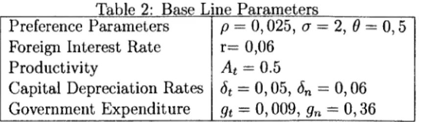
Mainly our calibration is based on the values of Morshed and Turnovsky (2004), however due to some differences on the models, we have changed a few parameters l.

We assume that the time discount rate is 0, 025 while the the world interest rate is set at 0, 06 and a takes value 2. This allow us to have a growth rate, 7, of 1.75 per cent which according to Brito and Correia (2000) is considered to be the long term rate of growth for the Portuguese economy. The share of traded good in the portfolio is 0, 5. Once that our productions functions are different from the ones of Morshed and Turnovsky (2004), we set the capital shares in order to have more realist results, that is Pt = 0,20, pn = 0,90 for

the case of det(B) > 0 and Pt — T 10, pn = 0,12 for reversed sign of the

B determinant2 The productivity parameter At takes value 0. 5 and will be

subject to shocks. gt and gn, the government consumption of traded and non-

traded good respectively, will take the values gt = 0,009 and gn = 0,36 and

will also be subject to shocks. We assume an adjustment cost for investment ^ = 15 which is on the superior limit for this type of parameter in aggregate

1 Some parameters were ehoose in order to obtain the elosest values for the benchmark

ratios of Morshed and Turnovsky (2004).

2Using these values, we will obtain the last case of table 2.1 which is also the most

common. AH other values equal, if we set pn = 0,93 we obtain the first case of table 2.1,

for pn = 0,92 we obtain the third case. We can have the second case for a very particular

parameter of pni smaller than 0, 93 and greater than 0, 92.

(35)

investment models,(see Auerbach and Kotlikoff (1987)). Finally, the depreciation rate for traded capital is set at ôt = 0,05, consistent with Brito and Correia (2000) and the depreciation rate for non-traded capital is ón = 0,06,

a bit superior 3. The baseline parameters are resumed in the following table:

Table 2: Base Line Parameters

Preference Parameters _{P = 0,025, a = 2, 0 = 0,5} Foreign Interest Rate V— 0,06

Productivity At = 0.5

Capital Depreciation Rates _{Ôt = 0,05, ô}n = 0,06

Government Expenditure _{9t = 0,009, g}n - 0,36

In order to make the interpretation clear, we linearized the expressions around the steady-state. The graphics represents percentage deviations from the initial steady-state and the vertical axes are in the same units to make horizontal comparatione clear.

4.2 Government Demand shocks

We assume that the government increase its demand for traded and non- traded good in one percentage point.

4.2.1 Case 1: det(/?)>0

3see Biorn et al. (1999) for estimations of depreciations rates.

(36)

Figure 1; Demand shocks for det(S)< 0 Increase in gt Increase in gn qtKl) 0 5 10 15 20 26 30 0 Tl r T I 1 I I I I I I I J TT~ 6 10 15 qtct) qtc») O 6 10 15 20 26 30 O 5 10 16 20 26 30 PfJ O 6 10 16 20 26 30 0,003 1 0.0026; 0.002' \ o 6 10 18 20 26 30 29

(37)

10 15 20 25 30 \ \ 10 15 20 t 25 30 10 16 20 26 30 10 16 20 26 30 10 16 20 26 30 10 15 20 25 30 \

As we can see the qualitative effects of both policies are basically the opposite. The government increases in traded good will crowd-out private consumption of traded and non-traded goods. As the demand for non-traded goods falis, its price will also fali so the relative price decrease. On the long run relative

(38)

price will return to its initial value. Trough a Stolper-Samuelson eífect, the relative price fali will increase the real reward of traded capital and decrease the real reward of non-traded capital, so it is not surprising that the traded capital stock rises, and the non-traded capital stock falis. Note that as the relative price reach its initial value the variations of the capital stocks are smaller. The variations of the capital stocks, provoke an increase on traded output and a decrease on non-traded output. This can be identified as a Rybczinsky effect.

The externai debt falis due to the increase on the traded sector output and a decrease in private consumption of traded good. To what concerns the GDP, in terms of traded good, there is a negative initial jump caused by the temporary depreciation of the relative price. The GDP will then follow a negatively sloped path towards its new steady-state value which is lower than the initial.

If the demand shock is made by a government consumption increase in non- traded good, the effect on the relative price is the opposite. When the government increases its demand for non-traded good, the price of these goods rises, so, the relative price rises too. While the relative price is above its steady-sate value we have once again the Stolper-Samuleson effect, that is, a relative price increase reduce the real reward of traded capital and rise the real reward of non-traded capital, thus the non-traded capital becomes relatively more attractive to investment so this stock will rise while the traded capital stock will fali.

Given the paths for the capital stocks, through the Rybczinsky effect, we know that traded output will fali and the non-traded output will rise. This time the initial jump of the GDP is positive and the new steady-state value is liigher 4. Note that the crowd-out effect on consumption that we saw when

the government increased its demand for gt will also be present for the case of

increase in gn. The externai debt, in the case that the government increases

its consumption on non-traded good rises.

4.2.2 Case 2: det(Í3)<0

In the case where traded sector uses more intensively non-traded capital, and the non-traded sector uses more intensively traded capital, a government

4 Note that for another parameter choice we could have different resulta

(39)

demand shock on gt and gn has the following effects 011 the economy 5.

Increase in gt

qb(t)

Figure 2; Demand shocks for det(/3)< 0 Increase in gn 10 15 20 25 30 0.4 10 16 20 26 30 Knct) 10 15 BO BB 30 -0.1 -0.2 10 16 20 26 30

5 Note that qt, p, and kt remain always on there steady state, therefore we have skipped

its figures.

(40)

X

O S 10 IS 20 25 ao

As we expected the effects are quite different from the previous case, both in qualitative and in quantitative terms. When gt rises, traded output has to rise to respond to the demand increase for this type of good. As traded sector is intensive in non-traded capital, firms will increase the non-traded capital stock in order to increase traded output. This increase in non-traded capital stock will have a negative effect on non-traded output (Rybczinsky effect). Traded capital stock remains at its initial value. Note that although trade sector's output rise, it is not sufficient to cover the demand increase so imports will rise therefore net externai debt will increase. In quantitative terras, the rise on traded output is greater then the negative effect on non- traded output thus the overall effect on the GDP is positive. Because the relative price does not change we do not have any initial jumps on the GDP in terms of the traded good.

If the government rises gn, the demand increase has to be fully satisíied by the

internai production once that it is impossible to import non-tradable goods. To fill the gap between supply and demand on the non-trade sector, that the policy has created, firms tend to deviate their production towards non-traded goods which causes traded output gradually to fali. Non-traded capital also falis with traded output (note that we are now working with the case where traded sector is relatively intensive in non-traded capital). Traded output falis more than non-traded output rises thus the effect on GDP is negative and externai debt falis.

(41)

4.3 Productivity Shocks

When a productivity shock occurs on the traded sector, the productivity of the non-traded sector is endogenously affected (see Proposition 1). Note that if we want to simulate a positive shock on the non-traded sector we can simply perform a negative shock on At.

The eíFects of a positive shock on At are given by:

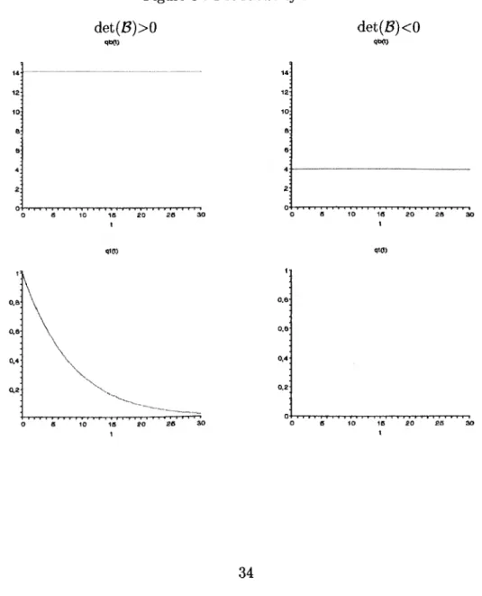
Figure 3 : Productivity shocks

det{Z3)>0 det(JS)<0

10 18 18 20 28

\

10 18 20 26 30 10 16 20 26 30

(42)

/ «o 16 20 26 l 10 16 20 26 M(t) s 10 15 20 26 30 Knft) 10 16 20 26 30 0,4 0.3 10 16 20 26 30 35

(43)

10 15 20 25 30 \

/

10 15 20 25

Starting by analyzing the left collum, it is clear that a productivity shock on traded sector will decrease private consumption. Remembering that we have a negative relation between At and An, we know that non-traded sector

productivity has decreased. The price of non-traded goods rise because this sector is now less efficient and the price of traded goods remain the same because it is tied to the international price of traded goods, as a result the relative price rise. Traded sector output rise, due to a higher productivity, therefore íirms have accumulate more traded capital and less non-traded capital. As it would be expectable the foreign debt falis because the economy is now more efficient. Looking at the right side collum where the analysis is made for the case of det{B) < O we can see that an increase in At will

also decrease private consumption. The relative price jumps immediately to a higher levei. Traded capital remains at its initial levei and non-traded capital stock rise to allow traded output to rise (note that in this case trade sector is intensive on non-trade capital).

Regarding the GDP, the supply shock causes a long run GDP higher than the original. This result is both for the case det{B) > O and det{B) < O, however as mentioned above, it could change for another parameter values.

(44)

Chapter 5

Conclusion

The main objective of this dissertation is to develop a two sector model of endogenous growth for a sinall open economy. In theoretical terms we found that positive growth is possible, however even 'ú r — p the existence of equilibrium is only verified for particular productivity parameters.

By having an explicit balance growth path, the model becomes stationary therefore we have an equilibrium point for the system, this allow us to study and understand the model dynamics around the steady-state in a very easy way.

We íind that the transitional dynamics for this model are saddle-path type in both the case of each sector more intensive in own capital, and the opposite case however the details of the local dynamics change, i.e. the dimension of the stable manifold is always one and the slope of stable manifold depends of the factor shares. Moreover the model show us that when det{B)> 0 there is a price adjustment and when det(jt?)< 0 there is a quantity adjustment, speciíically on non-traded capital.

The eífects of a productivity shock on traded sector are not independent of the factor intensities however the result on output of each sector is the expectable, traded output rises and non-traded output falis. In policy terms, we íind that demand policy can not aífect the relative prices on the long run, but an increase in government consumption of traded good will increase traded output and a government increase in non-traded good consumption will increase the output of non-traded sector. The overall eífect on the GDP is not clear.

This dissertation extends the endogenous growth literature, mainly AK models, by including two sectors and opening the economy. However the research

(45)

on this axea still has a few challenges. First it would be interesting extending this model with externalities and study the indeterminacy that will probably arise (basically what we are suggesting is solving Meng's model using our strategy). We think that would also be interesting to extend the present model adding a human capital sector, that is to develop a Uzawa-Lucas model of a small open economy with a tradable and a non-tradable sector. Finally the last challenge is to study the three sector model with externalities.

(46)

References

Auerbach, A. and Kotlikoff, L. (1987). Dynamic Fiscal Policy. Cambridge University Press.

Biorn, E., Lindquist, K., and Skjerpen, T. (1999). Micro data on capital inputs: Attempts to reconcile stock and flow information. Discussion Papers n 268, Statistics Norway, Research Department.

Bond, E., Wang, P., and Yip, C. (1996). A general two sector model of endogenous growth with human and physical capital: Banced growth and transitional dynamics. Journal of Economic Theory, 68:149-173.

Brito, P. (1999). Local dynamics for optimal control problems of three- dimensional ode systems. Annals of Operations Research, 89:195-214. Brito, P. (2003). Economia dinamica. ISEG/UTL, mimeo.

Brito, P. and Correia, I. H. (2000). Inflation diferential and real convergence in portugal. Banco de Portugal / Economic bulletin, ,;41-46.

Brito, P. and Pereira, A. (2002a). Convergent cyclical behavior in endogenous growth with housing. ISEG, UTL.

Brito, P. and Pereira, A. (2002b). Housing and endogenous long-term growth. Journal of Urban Economics, 51:246 271.

Gregorio, J. D., Giovannini, A., and Wolf, H. (1994). International evidence on tradables and non tradables inflation. European Economic Reviwe, 38:1225-1244.

Meng, Q. (2003). Multiple transitional growth paths in endogenously growing open economics. Jornal of Economic Theory, 108:365-376.

(47)

Morshed and Turnovsky (2004). Sectoral adjustment costs and real exchange rate dynamics in a twosector dependent economy. Journal of International Economics, 63:147-177.

Mulligan, C. and Sala-I-Martin, X. (1993). Transitional dynamics in two sector models of endogenous growth. The Quartley Journal of Economics, 108(3) :739-773.

Rebelo, S. (1991). Long run policy analysis and long run growth. Journal of Politicai Economy, 99:500-521.

Romer, P. (1986). Increasing returns and long run growth. Journal of Polit- icai Economy, 94:1002-1037.

Tu, P. (1994). Dynamical Systems. Springer-Verlag.

Turnovsky, S. (1996). Endogenous growth in a dependent economy with traded and nontraded capital. Review of International Economy, 4:300- 321.

Turnovsky, S. (2002). Growth in an open economy: Some recent develop- ments. In Smets, J. and Dombrecht, M., editors, How to Promote Eco- nomic Growth in the Euro Area. E. Elgar.

Wong, K. Y. (1997). International trade in goods and factor mobility. MIT Press.

(48)

Appendix

Demonstration 1

Let the Jacobian evaluated at steady-state leveis be denoted by Jc and let

jvUV = 1... 6, / = 1... 6 be the elements of the Jacobian, then we can write (45) as: where: 322 323 jss jl2 h\ 333 J55 jfí] Í62 j63 jtM ■ 0 0 0 0 0 0 " 0 722 J23 0 0 0 0 0 Jaa 0 0 0 0 Í42 0 0 0 0 3 31 0 3 33 754 333 0 . Jei Í62 333 J64 333 333 . 6 = r -7 J66 —jbA (Itn _ P kt 1 det{B) (1 ~ Pn){T + ôn) det{B) Pt (r + ôn mt rrin vQb da, ■nt , , d(ln1i K„ ■kt + dCn dp — r dp 1 dp dtn Ptf "b (l Prp^n p det{B) 7 7 Ct crqb Qtkt a P353 = (ítt + t 2^ 41

(49)

ík = '""="L(^(r+í")

The eigenvectors matrix (52) has the following shape: ^l1 í? 0 0 0 0 0 0 P3 0 _PI 0 0 0 0 0 P42 A3 0 1 P4 0 1 _n₃ _n₄ _n₅ 1 1 0 1 1 1 1 Where we assumed Ps — P3 and P" = P4.

Proof: Eigenvectors associated to A1/2 = 0, with multiplicity two. Solving (Jc — Ai/)?1 = 0 we obtain:

P1 = J54J22 _ 0 0

J51J64 — J61J54 JòljM ~ J61J54

As we have multiplicity two, the eigenvector associated with A2 is given solving (Jc — A2/)2P2 = 0

J54J65 - ■/55J64 q q JòbjGl ~ JblJôb ^ q jbijm - Jgi J54' ' ' Í51Í64 - jaijòi' Associated to A3 = ji'33 P3 = _0,^23^33 C/33 - J55) (J22 - J33) J33(.?33 - J55) O22 - jss)2 D D J42J23033 - Í55)(j22 - J33) [/53J33 (j22 - J33) - j42j,23Í54](j'"22 - jss) , D D where: // = Í23 (762 J33 + J64Í42 ) (J55 J33 ) -jfidas (.733 " jõõ ) (733 "722) -765753733 (733 -722) -765754742723 Associated to A4 = ,755 P4 = 0,0,0,0,^—^,1 765 42

(50)

Note that = jí66 — J33, substituting we obtain ^ so ^ ■'60

,765 Finally the eigenvectors associated to A5i6 = X = r - 7, with multiplicity two

are: J54 P0 = 0-01- ' jAl ' J55-Í22 ,1 p6 - 0 jggjjgS ~ ,722) q "(j55 — J22) -,1,1 J42J54 J54

because —^3— = where we calculated them doing (Jc —As/)?5 =

JOO J Á J 'w4J\JO '

0 for A5 and (Jc — Ag/)2?6 = 0 for the eigenvector associated with Ag ■

To find the sign of eigenvector P3, we star by writing their numerators as:

NPl = NP* NP* = NP* (p(r 7) 2(í(n)fl(Tlíinj P > 0 atnip{r - 7) - 2aín)(p(r - 7) - atn) p3 < 0 < o (p(r - 7) - 2atn)atnkt Cp jàsiatnCpjr - 7) - a2tnC] + kta2ntp2 Cf

As you can see the signs are ali clear except NP£. In this case we can identify a criticai value (J53J for which the sign changes. By solving NP* = 0 for 753 we obtain the criticai value.

J53c -

kt{antpf

íatn[p{r - 7) - a^]

For values of greater than we have a positive sign for the numerator of P5, for values smaller than j^c we will have a negative sign and for J53 = j^c

the numerator of is zero.

Knowing that the denominator is the same for ali Ff, í = 2,..., 5 and given by;

Z) = ai Ff + 0:2^53 + ttgSn (1)

(51)

where: ant(Mí(r - 7) - P^ní - ^í«ín) «1 = — zt vi (p{r - 7) - flínJCto «2 = Z < U V (p(r - 7) - 2atn)atn ^3 9 yra

We íind the criticai value ^53^ for the denominator by solving (1) to 753: . = p[(r - ^){atnÍCn + V0.ntkt<7qt) - {jxintfktcr ~ 2qtktantatncr] - 2a^{cn

■7j3'1 paiatn\p{r — 7) — otn]

Thus we can conclude that when ^53 > the denominator has negative sign, when j/53 — ^53^ the denominator is zero and finally when < j53d the

denominator has positive sign.

Demonstration 2

In order to calculated Jordan form associated with the Jacobian, we start by building the eigenvector matrix (see demonstration 1), then we pre multiply its inverse by the Jacobian and pos multiply it by (52). Jordan's form is, then given by;

0 0 0 0 0 0 0 0 0 0 0 0 0 0 A3 0 0 0 0 0 0 A4 0 0 0 0 0 0 _A5 0 0 0 0 0 0 Ae

Note that the equality . ^4. = jg cruciai for the shape of Jor-

n J J55-J22 Í42J05 r dan's matrix. Demonstration 3 Recall equation(54): x = — Jc S + (/ — J^Jc)/í 44

(52)

which are the long rim generalized multipliers that can be written as (58), that is: ~ Ki f'21 ^31 /■í41 + EÍ2 (h(Ki + k4 Mõl + Ef=l (p5(^e fJ-dl + ELl

In order to calculate the n vector, we start by calculating a generalize inverse of the Jacobian, = PJ^ P_1 then we multiply it for a generic S vector

and finally we obtain the // vector; 1 . Í23 ^21 + y—r—S31 96 Qt P k k-n b /^21 )"31 = -S31 /Ml Mõl + J22 J22J33 ]_ hz J42 , J42J23022 + J33) ^-521 H TT T-T^ «31 322 U22J33)2 _Í51 _ (j62j22 + J64J42)(.?22 - J55) , Numerator53 J55 11 J65O22J55)2 21 J65 (J22J33J55)2 31 (j22 — J55) (j62 J22 + jeijw) 1 "«41 —«51 /Ml = — J42J55J65

jssjei ~ hihbjjn + iss) (Í22J55)2 J55 «11 + ímj-nij-n + jss) + J64J42 (J22 + Í55) J55Í62 Numeratorw _ 762(^2 - Í55) + hthdv (./22J55J33)2 «31 Í22j42j25 «41 + (>22,755) 2 365 «21 322355 -«51 J22 «61 and: Numerator53 = 3^322325362 + jnhzjwhz - jh&hzjez + J23J42J55J64Í22 + jzzjwhzhhw+hzjwjeãhzhz — 322^5 j23h2js3 — JlshzhzjzAjw - hzjwjlsj eh zz Numeratorw = j^j^hzha + jhhzje^Jzz - J22J55J23J62 + 32235532z3623zz + J42j23j55j64j22 — 32235536Z3ZZ + 3ZZ34232Z364322 + 32235536535Z3ZZ — 355355325362 + j2zj42j55j64jZZ

(53)

Demonstration 4

Recall equation (57) which gives the paths for the variables after a shock. x{t) = í + PVq + P2/í2 + P8h3ex,t

Substituting the eigenvectors on the above expression we obtain;

Where: and Qb{t) = qb + Pl hi + Pfhi Qt{t) — Qt + P^h^e^1 p{t) - p + P^h3eX3t kt{t) = P*{eX3t-l)h3 kn(t) - P53(eA3t - l)/i3 h{t) - (eA3£-l)/i3 hi = [-kt + Pl~kn-{PlPl-Pl)b]~ h2 = [-pfkt-{Pl-P*)kn + PlPÍb] D' h, = [kt - Plkn - Plb] D' D' Pl + Pl Pl - Pl (3) (4) (5) (6) (7) (8) (9) (10) (11) (12)

Proof: Let P3 be a partition of the P matrix such that:

P3 =

Pl Pl Pl 0

1 o

1 Pi (13)

And let D' = Pl + P42 P^ — Pl be the determinant of the P3 matrix.

If we solve (57) for x{t) — x and evaluate for í = 0 we obtain:

1 ?r- O 1 ₁ ?s-: • ' hi ' knity kn = P3 62 6(0) - b . 'l3 . (14) 46

(54)

For the shake of simplicity we consider kt0 = kno = b0 = 0.

Solving (14) for h we obtain:

" /ll ■ " -kt ' /l2 — p-— *3 1

/l3 -b .

which are the values (9), (10) and (11). ■

substituting (58) on h\,h2,hz the expressions involving fae i = 4.. .6, i = 1... 4 cancel themselves which implies that the k vector is also canceled from the expressions and we find equations (65), (66), (67) and (68).

Let b be the long run multiplier for b, then we know that: 6(oo) = —h3 = b

Using this result on the system(3),... ,(8) we will obtain the system (59),... ,(64).

Demonstration 5

As the det(iB) < 0 then we will use Ps = P4 and = A4. The system (57)

is given by:

= Qb + Plh\ + Pyhi (16)

qt{t) - qt (17) p{t) - p (18) hit) = 0 (19)

knit) = /^(eA4f-l)h3 (20)

b{t) = (eA4Í - l)h3 (21) where: h = l-h + Pik - PtPfb)]~ (22) h = l-Píh)-Pik) + PiPm±; (23) h3 = [h) - Pfkn) - Pfb)]-^ (24) 47

(55)

and

D" - Pi + P42P54 (25)

Proof: As we saw, when det{B)<0 the stable eigenvalue is A4 and the asso ciated eigenvector is P4. Then the matrix P3 is now given by:

r p₄1 _Pl _0'

P3 = 0 1 PÈ (26)

1 0 1 The determinant of the matrix (26) is:

D" — Pl + P4P5 (27) Using the same method we used for the previous case we find the new values for the constants hi, ha and /13 given in equations (22), (23) and (24). ■

Substituting (58) on the system (16)... (21) we obtain the system (69)... (74).

(56)