Designs of Minimal-Order State Observer and
Servo Controller for a Robot Arm Using Piecewise
Bilinear Models
Tadanari Taniguchi, Luka Eciolaza, and Michio Sugeno
Abstract—This paper proposes a servo control system based on a minimal-order state observer for nonlinear systems ap-proximated by piecewise bilinear (PB) models. The design method is capable of designing the state observer and the servo controller of nonlinear systems separately. The approximated system is found to be fully parametric. The input-output (I/O) feedback linearization is applied to stabilize PB control systems. Although the controller is simpler than the conventional I/O feedback linearization controller, the control performance based on PB model is the same as the conventional one. The PB models with feedback linearization are a very powerful tool for the analysis and synthesis of nonlinear control systems. We apply the control method to a robot arm model. An example confirms the feasibility of the our proposals.
Index Terms—nonlinear control, piecewise bilinear model, input-output linearization, robot arm, minimal-order state ob-server
I. INTRODUCTION
P
IECEWISE linear (PL) systems which are fully para-metric have been intensively studied in connection with nonlinear systems [1], [2], [3], [4]. We are interested in the parametric piecewise approximation of nonlinear control systems based on the original idea of PL approximation. The PL approximation has general approximation capability for nonlinear functions with a given precision.One of the authors suggested to use the piecewise bilinear (PB) approximation [5]. PB approximation also has general approximation capability for nonlinear functions with a given precision. We note that a bilinear function as a basis of PB approximation is, as a nonlinear function, the second simplest one after a linear function. The PB model has the following features. 1) The PB model is derived from fuzzy if-then rules with singleton consequents. 2) It is built on piecewise hyper-cubes partitioned in the state space. 3) It has general approximation capability for nonlinear systems. 4) It is a piecewise nonlinear model, the second simplest after a PL model. 5) It is continuous and fully parametric. So far we have shown the necessary and sufficient conditions for the stability of PB systems with respect to Lyapunov functions in the two dimensional case [6], [7] where membership func-tions are fully taken into account. We derived the stabilizing Manuscript received December 23, 2013; revised January 30, 2014. This work was supported by a URP grant from Ford Motor Company which the authors thankfully acknowledge. In addition, this work was supported by Grant-in-Aid for Young Scientists (B: 23700276) of The Ministry of Education, Culture, Sports, Science and Technology in Japan.
T. Taniguchi is with IT Education Center, Tokai University, Hiratsuka, Kanagawa, 2591292 JAPAN, email: [email protected].
L. Eciolaza and M. Sugeno are with European Centre for Soft Computing, 33600 Mieres, Asturias, SPAIN, emails: [email protected], [email protected]
conditions [8], [9] based on the feedback linearization, where [8] applies the input-output linearization and [9] applies the full-state linearization. Although the controllers are simpler than the conventional I/O feedback linearization controller, the control performance based on PB model is the same as the conventional one.
This paper proposes a servo control system based on a minimal-order state observer of nonlinear control systems approximated by PB models. The design method is capable of designing the state observer and the servo controller of nonlinear systems separately. Although the controller is simpler than the conventional I/O feedback linearization controller, the control performance based on PB model is the same as the conventional one. In addition, the performance of the observer-based PB controller is equivalent to the PB controller without the state observer.
This paper is organized as follows. Section II presents the canonical form of PB models. Section III presents PB controllers for nonlinear plants with PB modeling and I/O linearization. Section IV presents a servo control of PB models. Section V proposes a minimal-order state observer for PB models. Section VI applies the proposed method to a robot arm model and shows the feasibility of the proposed methods. Section VII gives conclusions.
II. CANONICAL FORM OF PIECEWISE BILINEAR MODELS
A. Open-loop systems
In this section, we introduce the PB models suggested in [5]. We deal with the two dimensional case without loss of generality. Define a vector d(σ, τ) and a rectangle Rστ in the two-dimensional space as, respectively,
d(σ, τ)≡(d1(σ), d2(τ))T,
Rστ ≡[d1(σ), d1(σ+ 1)]×[d2(τ), d2(τ+ 1)].
σ and τ are integers: −∞ < σ, τ < ∞ where d1(σ) <
d1(σ+ 1), d2(τ)< d2(τ+ 1)andd(0,0)≡(d1(0), d2(0))T.
The superscriptT denotestransposeoperation. Forx∈Rστ, the PB system is expressed as
˙
x= σ+1
X
i=σ τ+1
X
j=τ
ωi
1(x1)ω2j(x2)f(i, j),
x= σ+1
X
i=σ τ+1
X
j=τ
ω1i(x1)ω2j(x2)d(i, j),
where
ωσ
1(x1) = (d1(σ+ 1)−x1)/(d1(σ+ 1)−d1(σ)),
ω1σ+1(x1) = (x1−d1(σ))/(d1(σ+ 1)−d1(σ)),
ωτ
2(x2) = (d2(τ+ 1)−x2)/(d2(τ+ 1)−d2(τ)),
ωτ+1
2 (x2) = (x2−d2(τ))/(d2(τ+ 1)−d2(τ)),
(2)
and ωi
1, ω
j
2 ∈ [0, 1]. In the above, we assume f(0,0) = 0
andd(0,0) = 0to guaranteex˙ = 0 for x= 0.
A key point in the system is that the state variablexis also expressed by a convex combination ofd(i, j)with respect to
ωi
1 andωj2 just as in the case ofx˙. As is seen in Eq. (2),x
is located inside Rστ which is a rectangle: a hypercube in general. That is, the expression of x is polytopic with four verticesd(i, j). The model ofx˙ =f(x)is built on a rectangle including xin the state space and it is also polytopic with four verticesf(i, j). We call this form of the canonical model (1) parametric expression.
Representingx˙ withxin Eqs. (1) and (2), we can obtain the state space expression of the model which is found to be bilinear (bi-affine) [5]. Therefore, the derived PB model has simple nonlinearity. In the case of the PL approximation, a PL model is built on simplexes partitioned in the state space, triangles in the two dimensional case. Note that any three points in the three dimensional space are spanned with an affine plane:y=a+bx1+cx2. A PL model is continuous. It
is, however, difficult to handle simplexes in the rectangular coordinate system.
B. Closed-loop systems
We consider a two-dimensional nonlinear control system. (
˙
x=fo(x) +go(x)u(x),
y=ho(x). (3)
The PB model (4) can be constructed from the nonlinear system (3).
( ˙
x=f(x) +g(x)u(x),
y=h(x), (4)
where
f(x) = σ+1
X
i=σ τ+1
X
j=τ
ωi1(x1)ω2j(x2)f(i, j),
g(x) = σ+1
X
i=σ τ+1
X
j=τ
ωi
1(x1)ωj2(x2)g(i, j),
h(x) = σ+1
X
i=σ τ+1
X
j=τ
ωi
1(x1)ωj2(x2)h(i, j),
x= σ+1
X
i=σ τ+1
X
j=τ
ωi
1(x1)ωj2(x2)d(i, j).
(5)
The modeling procedure in the region Rστ is as follows.
Algorithm 2.1: Piecewise bilinear modeling procedure 1) Assign verticesd(i, j)forx1=d1(σ),d1(σ+ 1),x2=
d2(τ),d2(τ+ 1) of the state vector x, then the state
space is partitioned into piecewise regions, see also Fig. 1.
2) Compute the verticesf(i, j),g(i, j)andh(i, j)in Eqs. (5), by substituting the values ofx1=d1(σ),d1(σ+1)
d1(σ)
d1(σ+ 1)
d2(τ)
d2(τ+ 1)
f1(σ+ 1, τ)
f1(σ, τ)
f1(σ, τ+ 1)
f1(σ+ 1, τ+ 1)
ωσ+1 1
ωσ 1
ωτ+1 2
ωτ 2
f1(x)
Fig. 1. Piecewise region (f1(x),x∈Rστ)
andx2=d2(τ),d2(τ+1)into original nonlinear
func-tionsfo,go andhoin the system (3). Fig. 1 illustrates the expression off1(x), wheref(x) = (f1(x), f2(x))T
andx∈Rστ.
The overall PB model can be obtained automatically when all the vertices are assigned. Note thatf(x),g(x)andh(x) in the PB model coincide with those in the original system at the vertices of all the regions.
III. DESIGN OFPBCONTROLLERS FOR NONLINEAR SYSTEMS WITHPBMODELING ANDI/OLINEARIZATION
This section deals with the I/O linearization of nonlinear control systems approximated with PB models. We consider, in particular, nonlinear systems and show their I/O lineariza-tion based on PB models in detail. First we give a brief introduction to the I/O linearization of PB models [9], [10].
A. I/O linearization
Consider the PB model (4) in the previous section. The derivativey˙ is given by
˙
y=∂h
∂x(f(x) +g(x)u) =Lfh(x) +Lgh(x)u.
where
Lfh(x) = σ2+1
X
i2=σ2 ωi2
2 · · ·
σn+1
X
in=σn ωin
n
h(δ1, i2, . . . , in)
d1(δ1)
f1+· · ·
+ σ1+1
X
i1=σ1 ωi1
1 · · ·
σn−1+1
X
in−1=σn−1 ωin
−1
n−1
h(i1, i2, . . . , δn)
dn(δn) fn,
Lgh(x) = σ2+1
X
i2=σ2 ωi2
2 · · ·
σn+1
X
in=σn ωin
n
h(δ1, i2, . . . , in)
d1(δ1)
g1+· · ·
+ σ1+1
X
i1=σ1 ωi1
1 · · ·
σn−1+1
X
in−1=σn−1 ωin−1
n−1
h(i1, i2, . . . , δn)
dn(δn) gn,
d1(δ1) =d1(σ1+ 1)−d1(σ1),
d2(δ2) =d2(σ2+ 1)−d2(σ2),
h(δ1, i2, . . . , in) =h(σ1+ 1, i2, . . . , in)−h(σ1, i2, . . . , in),
h(i1, δ2, . . . , in) =h(i1, σ2+ 1, . . . , in)−h(i1, σ2, . . . , in),
h(i1, i2, . . . , δn) =h(i1, i2, . . . , σn+ 1)−h(i1, i2, . . . , σn).
If Lgh(x) = 0, then y˙ =Lfh(x) is independent of u. We continue to calculate the second derivative of y, denoted by
y(2) and then we obtain
y(2)=∂Lfh
∂x (f(x) +g(x)u) =L
2
fh(x) +LgLfh(x)u, where
L2fh(x) =
∂Lfh
∂x1 f1+· · ·+
∂Lfh
∂xn
fn,
LgLfh(x) =
∂Lfh
∂x1
g1+· · ·+
∂Lfh
∂xn
gn,
∂Lfh
∂x1
= σ3+1
X
i3=σ3 ωi3
3 · · ·
σn+1
X
in=σn ωin
n
h(δ1, δ2, . . . , in)
d1(δ1)d2(δ2)
f2+· · ·
+ σ2+1
X
i2=σ2 ωi2
2 · · ·
σn−1+1
X
in−1=σn−1 ωin−1
n−1
h(δ1, i2, . . . , δn)
d1(δ1)dn(δn) fn
+ σ2+1
X
i2=σ2 ωi2
2 · · ·
σn+1
X
in=σn ωin
n
h(δ1, i2, . . . , in)
d1(δ1)
×
σ2+1
X
i2=σ2 ωi2
2 · · ·
σn+1
X
in=σn ωin
n
f1(δ1, i2, . . . , in)
d1(δ1)
+· · ·
+ σ1+1
X
i1=σ1 ωi1
1 · · ·
σn−1+1
X
in−1=σn−1 ωin−1
n−1
h(i1, i2, . . . , δn)
dn(δn)
×
σ2+1
X
i2=σ2 ωi2
2 · · ·
σn+1
X
in=σn ωin
n
fn(δ1, i2, . . . , in)
d1(δ1)
,
∂Lfh
∂xn =
σ2+1
X
i2=σ2 ωi2
2 · · ·
σn−1+1
X
in=σn
−1
ωin−1
n−1
h(δ1, i2, . . . , δn)
d1(δ1)dn(δn)
f1
+· · ·+ σ1+1
X
i1=σ1 ωi1
1 · · ·
σn
−2+1
X
in−2=σn−2 ωin−2
n−2
×h(i1, . . . , δn−1, δn) dn−1(δn−1)dn(δn)
fn−1
+ σ2+1
X
i2=σ2 ωi2
2 · · ·
σn+1
X
in=σn ωin
n
h(δ1, i2, . . . , in)
d1(δ1)
×
σ1+1
X
i1=σ1 ωi1
1 · · ·
σn−1+1
X
in−1=σn−1 ωin
−1
n−1
f1(i1, i2, . . . , δn)
dn(δn)
+· · ·
+ σ1+1
X
i1=σ1 ωi1
1 · · ·
σn−1+1
X
in−1=σn−1 ωin−1
n−1
h(i1, i2, . . . , δn)
dn(δn)
×
σ1+1
X
i1=σ1 ωi1
1 · · ·
σn
−1+1
X
in−1=σn−1 ωin−1
n−1
fn(i1, i2, . . . , δn)
dn(δn)
Once again, if LgLfh(x) = 0, then y(2) = L2fh(x) is independent ofu. Repeating this process, we see that ifh(x) satisfies
LgLifh(x) =0, i= 0,1, . . . , ρ−2, LgLρ −1
f h(x)6= 0 then u does not appear in the equations of y, y˙, . . .,
y(ρ−1) and appears in the equation of y(ρ) with a nonzero
coefficient:
y(ρ)=Lρ
fh(x) +LgLρ −1 f h(x)u.
The foregoing equation shows clearly that the system is input-output linearizable, since the state feedback control
u=(−Lρfh(x) +v)/LgLρ −1
f h(x)
reduces the input-output map toy(ρ)=v, which is a chain of
ρintegrators. In this case, the integerρis called the relative degree of the system.
IfLgLρ −1
f h(xt) = 0, the relative degree cannot be defined atx=xt. In some cases the relative degree can be defined at the point because we can adjust a partition of the state space for PB modeling so thatLgLρ
−1
f h(xt)6= 0.
Definition 3.1: The nonlinear system is said to have rela-tive degreeρ,1≤ρ≤n, in a regionD0⊂D if
LgLifh(x) = 0, i= 0,1,· · ·, ρ−2
LgLρ −1
f h(x)6= 0, for allx∈D0.
The input-output linearized system can be formulated as ( ˙
ξ=Aξ+Bv,
y=Cξ, (6)
whereξ∈ ℜρ,C= 1, 0, · · · , 0, 0T,
A=
0 1 0 · · · 0
0 0 1 . .. ... ..
. ... . .. ... 0
0 0 · · · 0 1
0 0 · · · 0 0
, B= 0 0 .. . 0 1 .
Note that all the feedback linearizable PB systems (4) are transformed into the linear system (6). Therefore it is easy to design the stabilizing controller and analyze stability of the PB systems.
According to the relative degree, three cases of linearized systems (6) must be considered.
• Relative degree:ρ=n
In this case, the state vector of the input-output linearized system is z = ξ = (h(x), Lfh(x), · · · , Lρ
−1
f h(x))T. The state vector z is necessary to be a diffeomorphism.
• Relative degree:ρ < n
There is unobservable state (n−ρ dimensions). It is necessary to consider the zero dynamics of the unob-servable stateµ. The state vector z is necessary to be a diffeomorphism. z = ξ, µT, ξ ∈ ℜρ, µ ∈ ℜn−ρ,
˙
µ(ξ, µ) =ζ1(ξ, µ) +ζ2(ξ, µ)v.µ˙(0, µ) is characterized
by zero dynamics. • In the case ofLgLi
fh(x) = 0,∀i, the proposed approach cannot be applied.
When the relative degreeρ≤n, the input-output linearizing controller isu=α(x) +β(x)v, where
α(x) =−Lρfh(x)/LgLρ −1
f h(x), β(x) = 1/LgLρ −1
system (6) can be obtained so that the transfer functionG=
C(sI−A)−1
B is Hurwitz.
The linearizing controller is also characterized as the LUT (Look-Up-Table) controller, where the LUT-controller is widely used for industrial applications, in particular, for vehicle control because of simplicity and also visibility as a nonlinear controller. In the case of the LUT-controller, control inputs are calculated by interpolation based on the table. When bilinear piecewise interpolation is adopted, the LUT-controller is found to be exactly the PB system.
IV. SERVOCONTROL
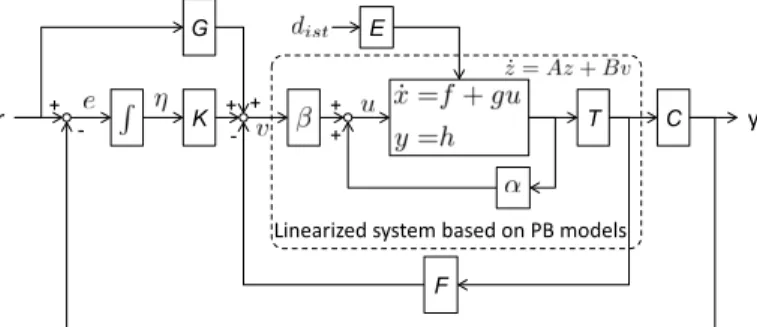
We apply a servo control [11] to nonlinear systems with the PB models based on I/O linearization. This is a two-degree of freedom servo control to nonlinear systems as shown in Fig. 2. The controller is designed to deal with disturbances and robustness. In this figure, T and R
show the coordinate transformation and the integrator. F,K, and
G are the feedback gains. r (r˙ = 0) is the setpoint signal anddist means a disturbance. Due to lack of space, we only discuss the nonlinear system with the relative degreeρ=n. The following approach can be also applied to the nonlinear systems withρ < n. We consider the linearized system using PB models.
( ˙
z=Az+Bv
y=Cz (7)
wherez∈ ℜn,A∈ ℜn×n,B∈ ℜn×m,v∈ ℜm,C∈ ℜl×n andy∈ ℜl. The control system is of a following form.
( ˙
z=Az+Bv,
˙
η=r−y, (8)
where the controller
v=−F z+Kη+Gr
is designed to make r−y →0 as t → ∞. We rewrite the system equations (8) as
˙
z
˙
η
=
A−BF BK
−C 0
z η
+
BG
1
r (9)
The gains of F andK are calculated such that the system (9) is stable. The gainGcan be obtained such thatz˙(∞) = 0 and y(∞) = r. Therefore the gain of G can be chosen
G=−(C(A−BF)−1B)−1. Finally, the two-degree freedom
servo controller is designed as
u=α(x) +β(x)v= −L ρ
fh(x)−F z+Kη−Gr
LgLρ −1
f h(x)
(10)
V. MINIMAL-ORDER STATE OBSERVER BASED ONPB MODELS
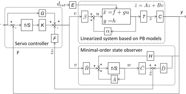
We proposed a full-order state observer of PB control system in [12]. In this paper, we propose an observer-based PB controller to estimate the minimal-order state z∈ ℜn−l by using the outputy∈ ℜl. Fig. 3 shows the minimal-order state observer for PB control system.
T C
F K
G
r + y
+ + +
- +
-
Linearized system based on PB models E
Fig. 2. Two-degree of freedom servo control system
The following system (11) is a minimal-order state ob-server, known as Gopinath observer [13].
( ˙
w= ˆAw+ ˆBv+Hy,
ˆ
z= ˆCw+ ˆDy (11)
where w ∈ ℜn−l, Aˆ ∈ ℜn−l×n−l, Bˆ ∈ ℜn−l×m, H ∈
ℜn−l×l,Cˆ ∈ ℜn×n−l,Dˆ ∈ ℜn×l andzˆ∈ ℜn−l.
The observer is designed by using the following steps [13], 1) Set a transformation T1 = [CT MT]T ∈ ℜn×n
satisfying detT1 6= 0, where M ∈ ℜn−l×n is an
arbitrary matrix.
2) A¯ andB¯ are divided as follows. ¯
A=T1AT1−1=
¯
A11 A¯12
¯
A21 A¯22
, B¯ =T1B=
¯
B1
¯
B2
where A¯11 ∈ ℜl, A¯12 ∈ ℜn−l×l, A¯22 ∈ ℜn−l×n−l,
¯
B1∈ ℜl andB¯2∈ ℜn−l.
3) Derive L ∈ ℜn−l×l so that Aˆ = ¯A
22 −LA¯12 is
Hurwitz.
4) Calculate the following parameters by usingL. ˆ
B=−LB¯1+ ¯B2, H = ˆAL+ ¯A21−LA¯11,
ˆ
C=T−1 1
0
In−l
, Dˆ =T−1 1
Il
L
.
The estimation zˆ of (11) is substituted into the servo con-troller (10), then the observer-based PB concon-troller is designed as
u=−L ρ
fh(x)−Fzˆ+Kη−Gr
LgLρ −1 f h(x)
,
˙
w= ˆAw+ ˆBv+Hy,
ˆ
z= ˆCw+ ˆDy.
Note that we can design the state observer for all the PB control systems. Since the linearized systems of all the PB models are the same as the linear system (7) and the system (7) is observable. In addition, the design method is capable of designing the state observer and the servo controller of nonlinear systems separately.
VI. ROBOT ARM MODEL
We consider a simple one-link robot arm [14]. The rotary motion is controlled by an elastically coupled actuator. The system is represented as
( ˙
x=fo(x) +go(x)u(x),
T C
F
r
y
+ + +
+ -
+ 1/S
H
+
+
Linearized system based on PB models
Minimal-order state observer
+
K G
1/S + +
-
y
Servo controller
E
Fig. 3. Minimal-order state observer and servo control systems based on PB models
The vectorsx,foandgo are given byx= (x1, x2, x3, x4)T,
fo(x) =
x3
x4
−K1
J1N2x1+
K1
J1Nx2−
F1
J1x3
K1
J2Nx1−
K1
J2x2−
mgd
J2 cosx2−
F2
J2x4
,
go(x) = 0, 0, 1/J1, 0T,
where x1 is the angle of the torsional spring on the gear
box and x2 is the angle of the robot arm. x3 and x4 are
the time derivatives of x1 and x2 respectively. J1 and J2
represent inertia,F1 andF2 are viscous friction constraints,
K1represents the elastic coupling with the joint andN is the
transmission gear ratio.m is the mass anddis the position of the center of gravity of the link.gis the acceleration due to gravity.
We choose the angle of the armx2 as the output, i.e.,
y=ho(x) =x2.
Now we divide the state-space of the robot arm model (12) as
x1∈{−15,15,15}, x2∈ {−5,5,5}, x4∈ {−5,5,5},
x3∈{−4π,−39π/10,−38π/10, . . . ,4π},
then the PB model is constructed as ˙
x=f(x) +gu, y=h(x) =x2
where
f1=
σ3+1
X
i3=σ3 ωi3
3(x3)f1(·,·, i3,·),
f2=
σ4+1
X
i4=σ4 ωi4
4(x4)f2(·,·,·, i4),
f3=
σ1+1
X
i1=σ1
σ2+1
X
i2=σ2
σ3+1
X
i3=σ3 ωi1
1(x1)ω2i2(x2)ωi33(x3)f3(i1, i2, i3,·),
f4=
σ1+1
X
i1=σ1
σ2+1
X
i2=σ2
σ4+1
X
i4=σ4 ωi1
1(x1)ω2i2(x2)ωi44(x4)f4(i1, i2,·, i4),
g= (0,0,0,1/J1)T,
f1(·,·, i3,·) =f1(j1, j2, i3, j4),
j1=σ1, σ1+ 1, j2=σ2, σ2+ 1, j4=σ4, σ4+ 1,
f2(·,·,·, i4) =f2(j1, j2, j3, i4),
j1=σ1, σ1+ 1, j2=σ2, σ2+ 1, j3=σ3, σ3+ 1,
f3(i1, i2, i3,·) =f3(i1, i2, i3, j4), j4=σ4, σ4+ 1,
f4(i1, i2,·, i4) =f4(i1, i2, j3, i4), j3=σ3, σ3+ 1.
Here f1(·,·, i3,·) is independent of i1,i2 and i4. It is also
the same forf2(·,·,·, i3),f3(i1, i2, i3,·)andf4(i1, i2,·, i4).
In this case, the system has many local PB models. Note that the linearized systems of the all PB models are the same as the linear system (7).
We design the servo controlleru
u=−L4fh/LgLf3h+ν/LgL3fh, (13) where
Lfh=f2(x), L2fh=f4(x), LgL3fh=
K1
J1J2N
,
L3
fh=
K1
J2N
f1(x) +
f2(·, σ2+ 1,·,·)−f2(·, σ2,·,·)
d2(σ2+ 1)−d2(σ2)
f2(x)
+−F2
J2
f4(x),
L4
fh=
K1
J2N
f3(x) +
f2(·, σ2+ 1,·,·)−f2(·, σ2,·,·)
d2(σ2+ 1)−d2(σ2)
f4(x)
+−F2
J2
−K
1
J2Nf1(x) +
−F2
J2 f4(x)
+ f2(·, σ2+ 1,·,·)−f2(·, σ2,·,·)
d2(σ2+ 1)−d2(σ2)
f2(x)
,
ν =−F z+Kη+Gr
=−(5.75,8.22,8.57,2.57)z+ 1.62η−5.75r.
The initial condition is x(0) = (0,0,0,0)T and the setpoint signal isr=π/2. The disturbance signaldist= 0.5 is added to the state x2 after 15 seconds. Fig. 4 shows the
state response of x2 using the PB servo controller with the
disturbancedist.
We construct a minimal-order state observer of this robot arm model. In this example we set a transformation T1 =
diag(1,1,1,1) and eigenvalues ρ1 = −200, ρ2 = −201,
ρ3 = −202 of Aˆ. The parameters of the observer (11) are
calculated as
L= 753, 1.89×10⁵, 1.58×10⁷T,
ˆ
A=
−753 1 0
−1.89×10⁵ 0 1
−1.58×10⁷ 0 0
, Bˆ=
0 0 1
,
ˆ
C=
0 0 0 1 0 0 0 1 0 0 0 1
, Dˆ =
1
−753
−1.89×10⁵
−1.58×10⁷
.
The estimation zˆ of (11) is substituted into the servo con-troller (10), then the observer-based PB concon-troller is obtain as
u= −L ρ fh
LgLρ −1
f h
+−(5.75,8.22,8.57,2.57)ˆz+ 1.62η−5.75r
LgLρ −1
f h
,
˙
w= ˆAw+ ˆBv+Hy,
ˆ
z= ˆCw+ ˆDy.
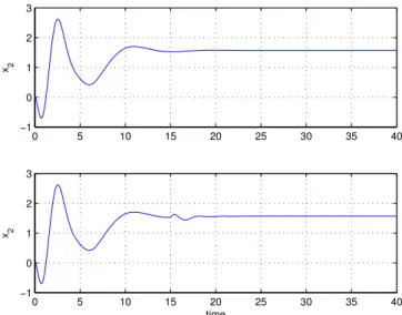
In Fig. 5, the upper graph shows the responses of the state
x2(t) without the disturbance and the lower one shows
the response with the disturbance. The results confirm the feasibility of the servo control and state observer. In addition, the results show that the controller has disturbance rejection feature. The performance of the observer-based PB controller is equivalent to the PB controller without the state observer.
0 5 10 15 20 25 30 35 40
−3
−2
−1
0 1 2 3
x2
Fig. 4. State responsex2using the PB servo controller with the disturbance
VII. CONCLUSIONS
This paper has proposed a servo control system based on a minimal-order state observer for nonlinear systems approximated by piecewise bilinear (PB) models. The design method is capable of designing the state observer and the servo controller of nonlinear systems separately. The approx-imated system is found to be fully parametric. The input-output (I/O) feedback linearization is applied to stabilize PB control systems. The PB models with feedback linearization are a very powerful tool for the analysis and synthesis of
0 5 10 15 20 25 30 35 40 −1
0 1 2 3
x2
0 5 10 15 20 25 30 35 40 −1
0 1 2 3
x2
time
Fig. 5. State responsesx2 using the observer-based PB servo controller
without/with the disturbance
nonlinear control systems. Although the controller is simpler than the conventional I/O feedback linearization controller, the control performance based on PB model is the same as the conventional one. We have applied the control method to a robot arm system. An example has confirmed the feasibility of our proposal.
ACKNOWLEDGMENT
The authors would like to thank Dr. Dimitar Filev and Dr. Yan Wang of Ford Motor Company for his valuable comments and discussions.
REFERENCES
[1] E. D. Sontag, “Nonlinear regulation: the piecewise linear approach,”
IEEE Trans. Autom. Control, vol. 26, pp. 346–357, 1981.
[2] M. Johansson and A. Rantzer, “Computation of piecewise quadratic lyapunov functions of hybrid systems,”IEEE Trans. Autom. Control, vol. 43, no. 4, pp. 555–559, 1998.
[3] J. Imura and A. van der Schaft, “Characterization of well-posedness of piecewise-linear systems,”IEEE Trans. Autom. Control, vol. 45, pp. 1600–1619, 2000.
[4] G. Feng, G. P. Lu, and S. S. Zhou, “An approach to hinfinity controller synthesis of piecewise linear systems,”Communications in Information
and Systems, vol. 2, no. 3, pp. 245–254, 2002.
[5] M. Sugeno, “On stability of fuzzy systems expressed by fuzzy rules with singleton consequents,”IEEE Trans. Fuzzy Syst., vol. 7, no. 2, pp. 201–224, 1999.
[6] M. Sugeno and T. Taniguchi, “On improvement of stability conditions for continuous mamdani-like fuzzy systems,” IEEE Tran. Systems,
Man, and Cybernetics, Part B, vol. 34, no. 1, pp. 120–131, 2004.
[7] T. Taniguchi and M. Sugeno, “Stabilization of nonlinear systems based on piecewise lyapunov functions,” in FUZZ-IEEE 2004, 2004, pp. 1607–1612.
[8] ——, “Piecewise bilinear system control based on full-state feedback linearization,” inSCIS & ISIS 2010, 2010, pp. 1591–1596.
[9] ——, “Stabilization of nonlinear systems with piecewise bilinear models derived from fuzzy if-then rules with singletons,” in
FUZZ-IEEE 2010, 2010, pp. 2926–2931.
[10] T. Taniguchi, L. Eciolaza, and M. Sugeno, “LUT controller design with piecewise bilinear systems using estimation of bounds for ap-proximation errors,”Journal of Advanced Computational Intelligence
and Intelligent Informatics, vol. 17, no. 6, 2013.
[11] ——, “Look-up-table controller design for nonlinear servo systems with piecewise bilinear models,” inFUZZ-IEEE 2013, 2013. [12] ——, “Full-order state observer design for nonlinear systems based
on piecewise bilinear models,” in2014 2nd International Conference
on System Modeling and Optimization, 2014, (accepted).
[13] B. Gopinath, “On the control of linear multiple input-output systems,”
The Bell Journal, vol. 50, pp. 1063–1081, 1971.