www.atmos-chem-phys.org/acp/5/169/ SRef-ID: 1680-7324/acp/2005-5-169 European Geosciences Union
Chemistry
and Physics
Comparison and evaluation of modelled and GOME measurement
derived tropospheric NO
2
columns over Western and Eastern
Europe
I. B. Konovalov1,2, M. Beekmann2, R. Vautard3, J. P. Burrows4, A. Richter4, H. N ¨uß4, and N. Elansky5 1Institute of Applied Physics, Russian Academy of Sciences, Nizhniy Novgorod, Russia
2Service d’A´eronomie, Institut Pierre Simon Laplace, Paris, France
3Laboratoire de M´et´eorologie Dynamique, Institut Pierre Simon Laplace, Paris, France
4Institute of Environmental Physics and Remote Sensing, IUP/IFE, University of Bremen, Bremen, Germany 5Institute of Atmospheric Physics, Russian Academy of Sciences, Moscow, Russia
Received: 8 September 2004 – Published in Atmos. Chem. Phys. Discuss.: 13 October 2004 Revised: 4 January 2005 – Accepted: 21 January 2005 – Published: 24 January 2005
Abstract. We present the results of a first comparison of the tropospheric NO2 column amounts derived from the
measurements of the Global Ozone Monitoring Experiment (GOME) with the simulated data from a European scale chemistry transport model (CTM) which is distinct from ex-isting global scale CTMs in higher horizontal resolution and more detailed description of the boundary layer processes and emissions. We employ, on the one hand, the newly devel-oped extended version of the CHIMERE CTM, which cov-ers both Western and Eastern Europe, and, on the other hand, the most recent version (Version 2) of GOME measurement based data-products, developed at the University of Bremen. We evaluate our model with the data from ground based mon-itoring of ozone and verify that it has a sufficiently high level of performance, which is expected for a state-of-the-art continental scale CTM. The major focus of the study is on a systematic statistical analysis and a comparison of spa-tial variability of the tropospheric NO2 columns simulated
with CHIMERE and derived from GOME measurements. The analysis is performed separately for Western and East-ern Europe using the data for summer months of 1997 and 2001. In this way, we obtain useful information on the na-ture and magnitudes of uncertainties of spatial distributions of the considered data. Specifically, for Western Europe, it is found that the uncertainties of NO2columns from GOME
and CHIMERE are predominantly of the multiplicative char-acter, and that the mean relative random (multiplicative) er-rors of the GOME measurement derived and simulated data averaged over the summer seasons considered do not exceed 23% and 32%, respectively. The mean absolute (additive) er-rors of both kinds of the data are estimated to be less than Correspondence to:I. B. Konovalov
3×10¹⁴mol/cm2. In Eastern Europe, the uncertainties have more complex character, and the separation between their multiplicative and additive parts is not sufficiently unambigu-ous. It is found, however, that the total random errors of NO2
columns from both GOME and CHIMERE over Eastern Eu-rope are not, on the average, larger than the errors of the NO2
columns with similar magnitudes over Western Europe.
1 Introduction
scale models for major populated regions contributes even-tually to validation of available emission data and, conse-quently, to better understanding of the chemical balance of the troposphere and the atmosphere in general. However, the extension of European CTMs beyond the Western Europe presents rather serious difficulties, because the amount of available observational data needed to specify model param-eters, and, especially, to validate model results outside West-ern Europe is rather limited. For example, only two stations out of more than 100 ones in the EMEP ground based ozone monitoring network are operating in Russia, and some other former USSR countries, e.g. Ukrainia and Byelorussia have no ozone measuring EMEP stations at all. The situation with measurements of ozone precursors in the mentioned coun-tries is even worse. Therefore, as far as modelling photo-oxidant air pollution over Eastern Europe is concerned, the traditional way of validation of continental scale CTMs via comparison of simulations with ground based observations of the key species (see, e.g. Fagerli et al., 2003) turns out to be of very limited utility.
Meanwhile, a significant source of global observational information concerning the atmospheric pollution, namely, satellite measurements of trace gases in the troposphere, has become available in recent years. It has been shown, in particular, that measurements performed by the satellite borne instrument of Global Ozone Monitoring Experiment (GOME) (Burrows et al., 1999) can be used to retrieve the tropospheric column amounts of nitrogen dioxide and sev-eral other trace gases (see, e.g., Velders et al., 2001; Richter and Burrows, 2002; Martin et al., 2002). More recently, the data retrieved from the measurements of the Scanning Imag-ing Absorption Spectrometer for Atmospheric Chartogra-phy (SCIAMACHY) featuring higher spatial resolution than GOME instrument have also become available (e.g. Buch-witz et al., 2004), but these data still have a preliminary and fragmentary character.
Although it is obvious, that comparison with NO2columns
cannot provide enough information about the overall model performance (concerning, e.g. predictions of ozone concen-trations), it may shed some light on the degree of uncertainty of input NOxemission data and of the quality of
representa-tion of major oxidarepresenta-tion and transport processes which play an important part in variability of other important photo-oxidants and their precursors. Besides, modelling of nitro-gen dioxide is important by itself, taking into account that NO2 plays an important part in the photochemistry of both
the boundary layer and free troposphere (see, e.g. Kley et al., 1999; Bradshaw et al., 2000) and contributes to radiative forcing of the climate (Solomon et al., 1999; Velders et al., 2001). Finally, comparison of simulated NO2columns and
those derived from satellite measurements may be helpful, in turn, for evaluation of the satellite measurement derived data, taking into account that the procedure of retrieval of tropospheric NO2 columns from satellite measurements
al-ways involves some a priori assumptions which are difficult
to validate, such as the shape of vertical profiles of tropo-spheric NO2, or the amount of scattering on aerosols.
The comparison performed within the framework of this study may be especially interesting from the last point of view particularly because we are the first to compare the latest version (Version 2) of the GOME measurement based data product for tropospheric NO2columns from the Bremen
University (http://www.doas-bremen.de/) with a CTM which was not used in the stage of retrieval of these data. The main difference between Version 2 and earlier Version 1 data is that Version 2 data were derived using tropospheric NO2
ver-tical profiles from the global CTM MOZART (Horowitz et al., 2003) while the constant profile with all NO2in a 1.5 km
boundary layer was assumed for Version 1 data. That is, on the one hand, it is reasonable to expect that Version 2 data are less uncertain than Version 1 data, but on the other hand, they are more dependent on performance of a certain model (MOZART). Therefore, a comparison of Version 2 data with corresponding data from another model is believed to be a really very useful step for evaluation of that new version of the satellite measurement based data.
This study addresses the following issues. First, we present the newly developed extended version of CHIMERE CTM, which covers the whole Europe and some neighbour-ing regions, and evaluate its performance over the whole do-main. In doing so, we present, to the best of our knowledge, first comparison of satellite measurement based data for tro-pospheric NO2 columns with calculations performed by a
continental scale CTM designed to study air quality issues. The advantages of our model over the global CTMs, with which the tropospheric NO2 columns derived from GOME
measurements were compared earlier (Velders et al., 2001; Lauer et al., 2002; Martin et al., 2003; Savage et al., 2004), are higher spatial resolution that matches well the resolution of GOME measurements in the South-to-North direction and more detailed parameterisation of the boundary layer pro-cesses. Our analysis is focused on statistical characteriza-tion and comparison of “fine” structure of spatial distribu-tions of the simulated and GOME measurement derived tro-pospheric fields of NO2. The comparison of model results
with satellite measurement data is supplemented by the com-parison of the simulated ground based ozone concentrations with those measured by the EMEP network and two stations of scientific atmospheric monitoring in Russia. On the one hand, the comparison of the simulated and observed ground based ozone concentrations allows us to demonstrate that CHIMERE features a sufficiently high level of performance expected for state-of-the-art continental scale models. And on the other hand, it is important in view of possible future applications of CHIMERE to study photo-oxidant pollution in Eastern Europe.
Second, we estimate the upper limits of spatially average random uncertainties (as distinct from systematic uncertain-ties equally applicable to all pixel considered) for both NO2
GOME measurements. Moreover, we make an attempt to characterise these uncertainties in terms of absolute (addi-tive) and relative (multiplica(addi-tive) errors. This issue seems to be especially important from the point of view possible application of satellite measurements for inverse modelling of emissions, because simulated NO2 columns are closely
linked to NOxemission data.
Finally, we pay special attention to the analysis of dif-ferences in statistical characteristics and uncertainties of the GOME derived and simulated NO2columns between
West-ern and EastWest-ern Europe. Such an analysis is very useful. In-deed, while emissions inventories for Western Europe have been extensively exploited and independently validated in numerous studies comparing results of continental and re-gional scale CTMs with observations (although in most cases not directly to NOxor NOy), the number and extent of
simi-lar studies concerning Eastern European countries is incom-parably smaller, because of a severe deficit of both models and observations. Recent comparisons of tropospheric NO2
columns derived from GOME measurements and those cal-culated by global models did not pay much attention to East-ern Europe, probably because the emission sources there are spread over vast territories, and, correspondingly, the average level of NO2pollution is much lower in Eastern Europe than
over such densely populated regions as Western Europe or South Asia. Nevertheless, it would be useful to note that, for example, total anthropogenic NOx emissions in Russia are
estimated to be considerably larger than those in any of the Western European countries taken alone (Vestreng, 2003).
The paper is organized as follows. The brief description of our version of the CHIMERE CTM is given in section 2, and its evaluation with data from the EMEP ground based ozone monitoring network is discussed in Sect. 3. Section 4 provides a description of the methods used to derive data for tropospheric NO2columns both from GOME
measure-ments and calculations by CHIMERE. Section 5 is devoted to comparison of the satellite measurement derived tropo-spheric NO2 columns with the corresponding simulated data, and Sect. 6 discusses the uncertainties of the analysed data. Finally, results of our study are summarised in Sect. 7.
2 Model description
This study is based on the use of the chemistry transport model CHIMERE which is an Eulerian multi-scale model designed for analysis of various air pollution related issues on urban and continental scales and for routine forecasting air pollution (http://prevair.ineris.fr). A description of basic features of the earlier version of the model can be found in the papers by Schmidt et al. (2001) and Vautard et al. (2001), and important recent updates are presented by Bessagnet et al. (2004). In-detail description of the model, the technical documentation and the source codes are available also on the web (http://euler.lmd.polytechnique.fr/chimere/). Therefore,
only those features which are the most important in the con-text of the given study or specific to our extended version of CHIMERE are mentioned below.
CHIMERE has been thoroughly evaluated both on the ur-ban scale for the Ile-de-France region (Vautard et al., 2001, 2003) and continental scale for Western Europe (Schmidt et al., 2001; Bessagnet et al., 2004). Although CHIMERE en-ables modelling of both gases and aerosols, this paper fo-cuses on gas-phase processes only.
The continental version of CHIMERE uses a rectangular grid with horizontal resolution of 0.5×0.5 degrees. The new CHIMERE domain used in this study is significantly larger (up to seven times) than any of the domains with which the model was used earlier. Specifically, it covers the region from 15◦W to 70◦E and from 25◦N to 70◦N, which in-cludes the whole Europe, Middle East, and a part of Northern Africa.
Meteorological input data for the CTM have been ob-tained from simulations with the non-hydrostatic meso-scale model MM5 (http://www.mmm.ucar.edu/mm5/) that has been run on a regular grid with horizontal resolution of 100×100 km. MM5 is initialised and driven with NCEP Re-Analysis data available on the web (http://wesley.ncep.noaa. gov/ncep data/) with a temporal resolution of 6 h and a spa-tial resolution varying from 1.8 to 2.5 degrees for different variables. MM5 is employed in order to compensate for this too low temporal and spatial resolution of NCEP data. Note that all previous studies with CHIMERE referenced above used ECMWF data with a horizontal resolution of about 50 km. Some “coarsening” of the standard configuration of CHIMERE proved to be inevitable in order to enable efficient simulations for the new larger domain.
In the vertical, the model has 8 layers whose heights are fixed using hybrid coordinates. The top of the upper layer is fixed at the 500 hPa pressure level. The fact that CHIMERE does not enable simulations of most of the free troposphere presents some limitation for our comparison of model calcu-lations with tropospheric NO2columns derived from GOME
measurements. However, this issue is not crucial, because, as is argued in Sect. 5, the spatial variability of tropospheric NO2 columns is determined mostly by lower tropospheric
NO2. Vertical diffusion is calculated within CHIMERE itself
using the parameterisation suggested by Troen and Mahrt (1986). Photolysis rates are calculated using the tabulated outputs from the Troposphere Ultraviolet and Visible model (TUV, Madronich and Flocke, 1998) and depend on altitude and zenith angle. The attenuation of radiation due to clouds is taken into account, based on the simplified assumption that the processes considered in the model take place below the top of the cloud layer. Correspondingly, the clear sky photol-ysis rates Jcare scaled with a radiation attenuation coefficient A which is calculated as a function of cloud optical depth; the actual photolysis rates are defined as a product A and Jc.
reaction rates. It includes 44 species and about 120 reac-tions and was derived from the more complete MELCHIOR chemical mechanism (Latuatti, 1997) using the concept of chemical operators (Carter, 1990; Aumont et al., 1997). Lat-eral boundary conditions are prescribed using monthly aver-age values of the climatological simulations by the second generation MOZART model (Horowitz et al., 2003).
The anthropogenic emissions are prescribed in essentially the same way as in the earlier studies with CHIMERE. Specifically, the annual EMEP data (Vestreng, 2003) for NOx, SO2, CO, and non-methane volatile organic
com-pounds (NMVOC) distributed to 11 SNAP sectors and grid-ded with horizontal resolution of 50×50 km are used to spec-ify emissions of corresponding model species for the most part of the new domain. But because dimensions of the new domain exceed sizes of the EMEP grid, the data from EDGAR V3.2 database (Olivier and Berdowski, 2001) are used to prescribe emissions for some territories (mainly, in Asia). These territories constitute only a minor part of the whole domain and are not the focus of this study. Daily, weekly, and seasonal variations of emissions were prescribed using data provided by the IER, University of Stuttgart (GENEMIS, 1994). As the new domain covers several time zones, the local administrative times were taken into ac-count. The annual NMVOC emissions were split first into emissions of 227 real individual hydrocarbons using typi-cal NMVOC profiles (Passant, 2002), and then emissions of these real species were aggregated into emissions of 10 NMVOC model species.
The land use data needed to parameterise biogenic emis-sions and dry deposition are obtained with a 1 km resolu-tion from the GLCF database (Global Land Cover Facility, Hansen et al., 2000, http://glcf.umiacs.umd.edu) and aggre-gated to the CHIMERE grid. Biogenic emissions of isoprene, pinene and NO are parameterised in accordance to method-ology suggested by Simpson et al. (1999), using distributions of tree species on a country basis provided in their work and the inventory of NO soil emissions by Stohl et al. (1996). The biogenic emissions for African and Asian countries (ex-cept Turkey and Kazakhstan) which are not covered in the cited inventories, are not taken into account, because they cannot be adequately described using the above mentioned methodologies designed for temperate regions. Simulations for these countries are anyway not the focus of this study and the paper’s conclusions are not affected by this omission.
3 Model evaluation with ground based observations
3.1 Observational data
While the main aim of this paper is comparison of model re-sults with data derived from satellite measurements, the com-parison with ground based measurements presented in this section plays a complimentary role and is intended, mainly,
to demonstrate that our version of CHIMERE performs rea-sonably well in a “classical” way of evaluation of continen-tal scale CTMs. Correspondingly, we do not consider here all available measurement data (that would be hardly possi-ble to do within a single paper anyway), but use mainly the data of ozone measurements from EMEP ground based mon-itoring network (http://www.nilu.no/projects/ccc/emepdata. html) for the years 1997 and 2001, and the data from two Russian ozone monitoring stations situated in remote re-gions and supervised by Institute of Atmospheric Physics (Moscow). These measurements are best suited to our goals, because, on the one hand, predictions of ozone concentra-tion, which, in the real atmosphere, depends on numerous physical and chemical processes, provide indeed a very seri-ous test for the model performance. And on the other hand, as the EMEP network is intended to reflect regional back-ground conditions relatively unaffected by local emissions of ozone precursors, the model resolution should be adequate at least for ozone.
Note that the measurements of other pollutants are less ap-propriate for comparison with our model. For example, in-sufficient resolution of the model’s grid is the most likely reason for a rather large disagreement between NO2
moni-toring data and continental scale models (see, e.g. Schmidt et al., 2001; Fagerli et al., 2003; Bessagnet et al., 2004). Such disagreement reflects, in particular, the well-known fact of a large spatial and temporal variability of that relatively short-lived species. Besides, the measurement and representative-ness errors are also considerable in the case of NO2(Aas et
al., 2000). Consequently, although along with the compar-ison with ozone measurements we have also performed the similar comparison with the ground based measurements of nitrogen dioxide, the results of that comparison are discussed in this paper only very briefly.
The EMEP ozone-measuring network includes 151 sta-tions. Normally, the hourly continuous measurements are re-ported. However, for some stations, the data were absent or incomplete for the periods that are considered in our study. Therefore, some selection criteria were needed. Specifically, only these days have been taken into account, for which the number of hourly measurements exceeded 18, and the sta-tions with data gaps for more than 30% of days in the peri-ods considered have been excluded from the analysis. As a result, for the summer period of 2001 considered below, we have selected 121 stations. Note that data from the major part of excluded stations (27 out of 30) are missing entirely for this period.
42.7◦E). Taking into account that data from only two ozone measuring EMEP stations in Russia are available for the pe-riods considered in this study, the data from even two more ozone monitors provide very substantial additional contribu-tion to available observacontribu-tional informacontribu-tion concerning East-ern Europe. To the best of our knowledge, no publications are available in which the data from these stations are com-pared with CTM simulations.
When ground based observations are compared with model results, it is necessary to define which model level cor-responds to a given station. The choice of the surface layer may be inappropriate for mountain sites where the model’s grid cannot resolve details of a relief. In this study, we chose an appropriate model level by considering the difference be-tween the actual height of a site (a.s.l.) and its height in the MM5 model topography (with resolution 100×100 km). Such a procedure is believed to be the most unambiguous, al-though it does not provide a general solution for the problem of low resolution of a model in mountainous areas where the performance of the model may be worse than over plains. 3.2 Results
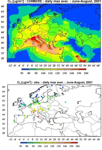
Figure 1 presents a simulated distribution of mean daily maximums of ozone concentrations over model domain in comparison with the corresponding observed data. Note that simulated ozone concentrations are given for the lowest CHIMERE level, and only these stations are shown which, in accordance to the criterion discussed above, correspond to this level. Although it is difficult to judge about adequacy of the simulated ozone distribution based on comparison with the given very fragmentary observational picture, it is use-ful to note that both observations and measurements mani-fest the pronounced north-to-south gradient of ozone concen-tration. Such gradient appears to be quite a reasonable fea-ture of the simulated ozone field taking into account that the stronger insolation and higher temperatures facilitate faster ozone production in densely populated regions in Southern Europe when compared with the similar regions in North-ern Europe. Considering variability of ozone concentrations in the West to East direction, it can be noticed that both the model and observation show larger concentration over Ger-many and Italy than over England, Spain and Portugal in the West and Poland and Slovakia in the East. The high level of simulated ozone concentration over Mediterranean Sea and Persian Gulf is, probably, a result of a combination of large emissions of ozone precursors from surrounding coastal ar-eas, strong radiation, and a low rate of ozone deposition on a water surface. Note also that the mean level of modelled ozone pollution is generally lower over Eastern than Western Europe in agreement with the lower population density and associated emissions of ozone precursors in Eastern Europe. In order to quantify the model performance in capturing spa-tial structure of the measured mean ozone concentrations, we have evaluated the correlation coefficient between the mean
Fig. 1.Spatial distributions of daily maximum average ozone con-centrations calculated by CHIMERE and observed at stations of the EMEP monitoring network.
observed and measured ozone concentrations for all sites. It equals 0.70.
Let us further consider several classical statistics used for evaluating air quality models. These are the standard corre-lation coefficient,R, the normalized root mean square error,
N RMSE=
1 N
PN
i=1(Cim−C o i)
2
¯
Co
1/2
, (1)
and the mean normalized bias, BI AS=
¯
Cm− ¯Co
¯
Co . (2)
Here,CoandCmare observed and modelled daily maximum concentrations at a given location, andC¯oandC¯mare their averages over the considered periods.
Fig. 2.Comparison statistics for daily maximums of ozone concen-trations simulated by CHIMERE and measured by ground based ozone monitors.
average of 62%. Persistently high correlations are typical for Germany, Belgium, and the Netherlands, and generally smaller ones are found for the sites in Eastern and Northern Europe. This may be indicative of the fact that CHIMERE works best for the sites situated in relatively polluted environ-ments where ozone behaviour is determined by photochemi-cal processes rather than the long-range transport.
However, it is important to note that even when the model performs badly in terms of correlation coefficient, it still may
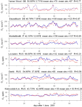
Fig. 3. Time series of daily maximums of ozone concentrations (mixing ratios) for summer season 2001. Solid lines and crosses show model results and observations, respectively. Note that the data are presented in original units of measurements for a given station.
perform quite satisfactory with regard to normalized RMSE. For example, a very small correlation coefficient (29%) and a rather low NRMSE (18%) co-exist for the Kislovodsk high-mountain station. A similar behaviour is observed also for many other remote stations both in North and South of Eu-rope. As the day-to-day variability of ozone concentration is relatively small at these sites, the errors of model predic-tions, which may be large when compared with the variance of the measured data, look small when compared with the mean value of ozone concentration. Taken on the average for all the sites, the NRMSE is found to be about 24 percent.
Biases are in the range from−20 to 20 percent for most of the sites. Their absolute magnitudes are less than 10% for 53 out of 121 sites considered, and less than 15% for 84 sites. When averaged over all the sites, the mean bias is slightly positive (about 7 percents).
RMSE, and the mean bias are found to be 65, 25, and 6 (44, 22, and 7) percent, respectively. As it has already been noted above, the relatively high correlations are typical for the sites located within highly urbanized regions, which are character-istic of Western Europe rather than of Eastern Europe. Corre-spondingly, the differences in the model performances with respect to the correlation coefficients cannot be considered as sufficiently strong evidence in favour of better quality of ozone simulations by CHIMERE for Western Europe when compared to those for Eastern Europe. It should be empha-sised also that the statistics reported above for Eastern Eu-rope are likely not quite representative of the whole of East-ern Europe because they are based on a very limited number of stations.
Figure 3 presents examples of simulated and observed time series of ozone daily maximums for several sites in Western Europe and Eastern Europe (Russia). It is interest-ing to note that the largest differences are observed durinterest-ing the episodes of elevated ozone concentrations, even if they are generally well pronounced in simulations, too. Among the sites presented in Fig. 3, the model performs worst at Lovozero. However, on the one hand, the typical ozone mix-ing ratio observed at this remote site is very low, and so the absolute errors of model predictions are not very large when compared with the other sites. On the other hand, Lovozero is situated almost on the edge of the model domain and thus the simulated results may depend strongly on the boundary conditions.
The statistics considered above, when taken alone, do not enable conclusions about model performance to be drawn in qualitative terms such as “good” or “bad”. Therefore, it would be useful to compare our results with the corre-sponding results of other European continental scale models. For such a purpose, we consider here the results of model evaluations presented in the Special Report to EUROTRAC (Roemer et al., 2003). Table 1 lists the comparison statistics for daily maximums of ozone concentration, obtained with several continental scale models for different measurements sites. Note that while not all of the sites considered in the Special Report belong to EMEP monitoring network, only EMEP sites are considered here. All the models, including ours, were run for the period from 1 May to 31 August 1997. It seems to be evident that although the performance of our version of CHIMERE is, to some degree, worse than the per-formance of the “standard” CHIMERE, it still equals on the average the performances of the other models.
The comparison statistics defined above were evaluated also using NO2near-ground daily mean concentrations
sim-ulated by CHIMERE and those measured at EMEP stations for three summer months of 1997. The values of the corre-lation coefficient, the normalised RMSE, and the mean bias averaged over 53 stations selected using the same criteria as in the case of ozone measurements are found to be 20, 80, and−19 percent, respectively. Although these results look significantly worse than similar results for ozone, the large
discrepancies between observations and simulations in this case are caused, most probably, by the reasons mentioned in the previous section (insufficient spatial resolution of the model in case of such a short-lived species as NO2and
sig-nificant measurement errors) and do not mean that NO2data
from CHIMERE are indeed of very low quality. In fact, the output data from CHIMERE represent NO2
concentra-tions averaged over a grid cell and, therefore, it would be best to compare them to measurement data representing the similar scales. Such kind of data can be provided by satel-lite measurements, which, for that reason, seems to be much more suitable for evaluation of CHIMERE and other simi-lar models than in situ measurements of NO2. On the other
hand, the disagreement with NO2 ground based
measure-ments does not look so large if we consider spatial correlation between simulations and measurements averaged over sev-eral months. Specifically, we have found that for the period indicated above, the respective correlation coefficient equals 0.82.
Finally, considering all the results presented in this section, we can conclude that our extended version of CHIMERE is a state-of-the-art continental scale model which simulates spatial-temporal evolution of near-ground ozone concentrations satisfactorily in Western, Central, and Northern Europe. However, the available ozone measure-ments do obviously not enable correct evaluation of the model performance for the major part of Eastern Europe, nor for Northern Africa and Middle East, for which no surface observations were available in this work. The comparison of the model results with the data derived from the GOME mea-surements, which is discussed in the next sections, provides substantial additional information on model performance in Eastern, as well as in Western Europe.
4 Description of tropospheric NO2data
4.1 Tropospheric NO2 columns retrieved from GOME
measurements
We use the most recent version (Version 2) of tropospheric NO2 column data products that were created at the
Table 1.Comparison statistics calculated for daily maximums of ozone concentrations observed at EMEP stations and simulated by European scale chemistry transport models for the period from 1 May to 31 August, 1997. The results for the standard version of CHIMERE and other models are listed in accordance to Roemer et al., 2003.
R, % NRMSE, % BIAS(%)
chimere1 chimere2 other models avg.3 chimere1 chimere2 other models avg.3 chimere1 chimere2 other models avg.3,6
vredepeel nl 84 81 72 20 35 31 20 20 10
eupen be 80 80 70 29 29 28 17 13 5
deuselbach de 85 84 67 15 18 23 6 2 11
brotjacklriegel de 77 81 51 23 12 23 −2 1 14
payerne ch 79 68 67 15 29 19 4 18 8
illmitz at 68 62 55 14 17 22 −4 0 12
ispra it 56 43 39 25 29 33 −13 11 18
aston hill uk 64 62 47 49 36 46 39 12 22
harwell uk 70 78 66 28 26 32 13 −3 10
sibton uk 69 86 60 31 20 33 2 1 12
yarner wood uk 68 71 58 33 26 38 23 4 20
eskdalemuir uk 71 79 62 42 23 31 33 3 14
mace head ie 68 68 60 15 27 27 2 −15 7
average4,6 72 73 60 26 25 30 14 8 13
birkenes no 51 nd 38 23 nd 27 10 nd 9
jeløya no 52 nd 45 19 nd 23 3 nd 10
r¨orvik se 63 nd 47 18 nd 23 10 nd 10
ut¨o fi 36 nd 39 18 nd 26 3 nd 14
vindeln se 51 nd 42 25 nd 28 2 nd 10
esrange se 45 nd 45 23 nd 33 −8 nd 23
aliartos gr 20 14 10 20 nd 27 5 nd 12
noia es 69 65 44 16 24 31 3 −19 14
san pablo es 61 nd 34 14 nd 24 −9 nd 15
preila lt 52 44 47 24 21 27 14 6 14
starina sk 48 47 36 20 31 25 6 25 6
kosetice cs 73 65 52 13 16 24 −2 0 13
k-puszta hu −23 −26 −21 31 28 34 −21 −15 25
average5,6 46 nd7 35 20 nd7 27 7 nd7 13
1the current version of CHIMERE,
2the standard Western European version of CHIMERE participated in the study by Roemer et al. (2003),
3 the average over other European models (NILU-CTM, EUROS, MATCH, LOTOS, EURAD, REM3/CALGRID, DEM, STOCHEM,
DNMI) participated in the study by Roemer et al. (2003), 4average over stations from Vredepeel to Mace Head, 5average over stations from Birkenes to K-puszta,
6for biases, the averages over their absolute values are given, 7not enough data
of some other gases, including NO2, by means of the
Dif-ferential Optical Absorption Spectroscopy (DOAS) method (Richter, 1997, see also http://www.doas-bremen.de/). ERS-2 has a sun-synchronous near-polar orbit with an equator crossing time of 10:30 LT in the descending node. The typi-cal ground pixel size is 320 km across the track (i.e. in West-East direction), and 40 km along the track. The nearly global coverage is reached in 3 days.
It is important to note that the information provided by GOME measurements is sufficient for retrieval of only
to-tal atmospheric NO2slant columns. In earlier version
(Ver-sion 1) of data products of the Bremen University group, the tropospheric NO2columns were evaluated further using
the tropospheric excess method introduced by Richter and Burrows (2002). That method was based on the estimation of stratospheric NO2slant columns using total atmospheric
NO2columns in remote parts of the oceans and the
assump-tion of homogeneity of longitudinal distribuassump-tion of strato-spheric NO2. In Version 2 data, a longitudinal variability
simulations with the global CTM SLIMCAT (Chipperfield et al., 1999) sampled in the time of GOME overpass.
The tropospheric NO2columns are then derived from the
tropospheric slant columns by applying the pre-calculated air mass factors (AMF) which prescribe an effective path of light in the troposphere and depend, in particular, on ver-tical distribution of the absorbing gas, aerosol and clouds in the troposphere, and on solar zenith angle and surface albedo. Different approaches and assumptions to evaluate air mass factors were used in different versions of data prod-ucts of IUP. In particular, Version 1 data (see, e.g. Richter and Burrows, 2002; Lauer et al., 2002) were derived under simplified assumptions that all tropospheric NO2is
homoge-neously distributed (in vertical) below 1.5 km. The retrieval of Version 2 data is based on the use of monthly averaged AMF evaluated with NO2 profiles from the global model
MOZART for the year 1997 (Horowitz et al., 2003, see also http://www.mpimet.mpg.de/en/extra/models/mozart/).
Other major improvements concern the evaluations of cloud parameters and surface albedo, which are obtained from GOME measurements using the algorithms discussed by Koelemeijer et al. (2001) and Koelemeijer et al. (2003). Note that cloud parameters are needed to select the pixels with low cloud cover; a cloud cover threshold equal 0.2 is used in the retrieval of Version 2 data, and no further cor-rection of AMF due to clouds is performed. Version 1 data will not be further discussed in this paper, although it seems worthwhile to note that the comparison of NO2columns
sim-ulated with CHIMERE with these data were also performed in the preliminary stage of our study. A disagreement be-tween model results and Version 1 data was found to be sig-nificantly larger than in the case with Version 2 data that may be indicative of larger uncertainty of Version 1 data. 4.2 Simulated NO2columns
We use the model data corresponding to summer seasons of 1997 and 2001. The choice of the year 1997 has been al-most obvious, taking into account that evaluation of AMF used for the retrieval of tropospheric NO2 columns from
GOME measurements were based on MOZART run for this year and, consequently, the respective GOME data are ex-pected to be more consistent than the data for any other year. The year 2001 is considered mainly in order to get an idea of a degree to which our estimations may be sen-sitive to inter-annual variability of tropospheric NO2. The
choice of summer months has been pre-determined by the fact that CHIMERE is designed, primarily, for simulating photo-oxidant pollution that is usually strongest during the warm season. Besides, the uncertainty of GOME data may be larger for other seasons due to larger cloud cover and pos-sible strong reflection from ice and snow.
In order to be consistent with GOME derived data, the modelled NO2 columns for each model grid cell are taken
in local solar time between 10 and 11 h and only on days
with insignificant cloud cover. Because the total cloud cover is not considered in CHIMERE, we use a selection criteria based on a 0.7 threshold value of the radiation attenuation coefficient, which corresponds to 30% reduction of solar ra-diation due to clouds. We tested the sensitivity of simulated monthly average NO2 columns to the radiation attenuation
coefficient threshold value and found that it is very insignifi-cant. Note also, that whatever a criterion was used, the selec-tion of “good” days and pixels out from the simulated data could not be done quite consistently with the procedure em-ployed for retrieval of GOME data because of the use of dif-ferent meteorological data.
The daily data for simulated NO2columns are combined
in order to obtain monthly averaged distributions that can be used for comparison with the data-products for monthly mean NO2 columns derived from GOME measurements.
Also, in order to provide better similarity of horizontal reso-lution of simulated and GOME derived data, CHIMERE data has been preliminary averaged for each 7 consecutive grid cells in West-East direction. Note that CHIMERE grid used in this study is exactly the same as the grid used in Version 2 NO2data-products. Note also that although our version of
CHIMERE is capable of simulating only lower tropospheric NO2columns (up to 500 hPa pressure level), we use
evalua-tions of tropospheric NO2columns above 500 hPa, obtained
using the same output database of the global CTM MOZART that is used to prescribe boundary and initial conditions for CHIMERE (see Sect. 2).
5 Overview and comparison of GOME retrieved and simulated NO2distributions over the model domain
Figure 4 presents distributions of tropospheric NO2columns
derived from GOME measurements, lower and upper tro-pospheric NO2column amounts simulated with CHIMERE
(below 500 hPa) and MOZART (above 500 hPa), respec-tively, and combined (CHIMERE plus MOZART) total tro-pospheric NO2columns; all the data shown are averages of
June to August monthly means. Seasonally averaged dis-tributions rather than data for individual months not only enable more concise presentation and discussion of our re-sults, but it is also very reasonable to consider them from the point of view of potential applications of our results for in-verse modelling of emissions. Indeed, averaging of modelled and observational data over summer period enables a dras-tic reduction of the “random” errors of the data, and, con-sequently, obtaining more consistent relationships between emission fields and NO2columns. Note that the data from
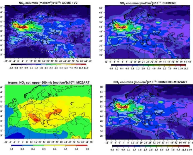
Fig. 4.Distributions of tropospheric NO2columns derived from GOME measurements in comparison with lower tropospheric NO2columns (above 500 hPa pressure level) simulated with CHIMERE, upper tropospheric NO2 columns evaluated with MOZART, and composed (CHIMERE plus MOZART) total tropospheric NO2columns. The GOME and CHIMERE data represent the averages over the summer months of 1997. Upper tropospheric NO2were evaluated by averaging monthly NO2MOZART data corresponding to the summer of 1996. Note differences in scales of the plots.
It is seen in Fig. 4 that many similarities exist between GOME measurements and simulated lower and total tropo-spheric NO2 columns. In particular, both kinds of data
ex-hibit the strongly enhanced NO2 columns over the Great
Britain, Belgium, Netherlands, and North-western Germany; some other polluted areas, such as Po Valley in Italy and Moscow region in Russia, are well pronounced. Both CHIMERE and GOME data indicate much lower level of air pollution in Eastern Europe compared to Western Europe. However, along with similarities, there are a number of dif-ferences. For example, GOME measurements give signifi-cantly larger values of NO2columns over Israel and Persian
Gulf region than predicted by the models, but the reverse situation is observed, in particular, over areas at Southern Poland and around Moscow.
It is very important to note that, as evidenced by the MOZART data, the contribution of upper tropospheric NO2
to the total tropospheric NO2columns is rather small over the
most part of Western Europe. The relative contribution of the upper troposphere is more significant over Eastern Europe; nevertheless, as it can be seen in Fig. 4, spatial variations of both NO2 columns derived from GOME measurement and
those simulated by CHIMERE are generally much stronger than spatial variations of the upper tropospheric NO2.
Figure 5 presents distributions of NO2 columns derived
from GOME and simulated by CHIMERE for summer of 2001. A comparison of Figs. 4 and 5 indicates that inter-annual variability of NO2 columns is not large, although it
can hardly be neglected completely. More careful examina-tion of differences between 1997 and 2001 in the modelled and GOME measurement derived NO2columns reveals that
they correlate very badly (R<0.2) and that the average (over the whole model domain) decrease of NO2column amounts
Fig. 5.Distributions of the tropospheric NO2columns derived from GOME measurements in comparison with the lower tropospheric NO2 columns simulated by CHIMERE. The data shown represent the averages over summer months of 2001.
data (0.1%). The last observation indicates that the EMEP emission database may overestimate an actual reduction of the anthropogenic NOx emissions. However, this
supposi-tion needs further careful analysis that is beyond the scope of this paper.
In order to enable a statistical analysis of differences be-tween Western and Eastern Europe, we define two regions, one of which is restricted between 10◦W, 18◦E, 35◦N and 60◦N, and another between 18◦E, 65◦E, 40◦N and 65◦N. These regions will be referred to in the following as to West-ern and EastWest-ern Europe, respectively. Although such a defi-nition does not follow exactly any political boundaries, nev-ertheless, such defined regions seem to be well representative of more densely populated industrial regions in Western and Central Europe on the one hand, and less urbanized countries in Eastern Europe on the other hand.
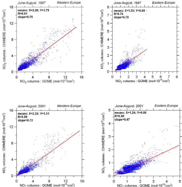
Figure 6 presents the scatter-plots of simulated and GOME measurement derived NO2columns for Western and Eastern
Europe. It is seen that the correlations are rather significant, although the scatter is also substantial. The agreement is ap-parently better for Western Europe; however, it is necessary to take into account the differences in scales of variability of the data for the two regions. The better correlations for West-ern Europe may stem simply from the fact that the range of possible magnitudes of NO2columns at Western Europe is
much larger when compared to Eastern Europe. The differ-ences between the considered regions are discussed in more details in the next section.
It is noteworthy that the slopes of the linear fits are con-siderably less than unity in all cases shown in Fig. 6. It is indicative of significant systematic errors in, at least, one of the considered datasets, whose magnitudes are dependent on the amplitude of the NO2 columns. It is interesting to
note also that a few points corresponding to values above 3×10¹⁵mol/cm2in Eastern Europe look as if they were out-liers, especially in the case of 1997. They correspond to the
areas about Krakow in Poland and Moscow in Russia. This observation may be indicative of overestimated NOx
emis-sions prescribed in CHIMERE for these two areas. This over-estimation is, probably, much stronger in the EMEP emission database for 1997 than for 2001. Anyway, our suggestion concerning overestimated NOxemissions about Krakow and
Moscow is the hypothesis that yet needs to be proved in a further special research.
Table 2 lists the basic statistical characteristics of the dis-cussed data for different months and years. Estimates of con-tributions of upper tropospheric NO2 are given in Table 3.
It is easy to see that the means of CHIMERE and GOME data agree for Western Europe within less than 32% of un-certainty (relative to the mean of the GOME retrievals) for all months considered in 1997. The negative difference between the means of the CHIMERE and GOME NO2 columns is
larger in 2001 and reaches 41% in August. The larger differ-ence in 2001 is, mainly, due to the reduction of NO2column
amounts in CHIMERE data in that year (compared to 1997), which is not found in GOME data. The consideration of the results given in Table 2 together with the estimates provided in Table 3 reveals that a considerable part of the noted dis-crepancies can be explained by the unaccounted contribution of the upper tropospheric NO2in CHIMERE NO2columns.
Fig. 6.Scatter plots of the simulated and GOME derived NO2columns for Western and Eastern Europe.
modelled NO2 vertical profiles that have been used to
cal-culate the modelled NO2 columns, while the vertical NO2
profiles that have been used to elaborate Version 2 data-products considered here are different from those obtained from CHIMERE. In our case, there is therefore a greater chance that systematic errors of the modelled and GOME measurement derived NO2columns have the same sign and
similar magnitude. Nonetheless, an important advantage of our approach is that the random errors of the NO2 columns
from CHIMERE and GOME can be assumed to be statisti-cally independent. This advantage is exploited in the next section.
As to Eastern Europe, CHIMERE gives about a factor two lower mean values than those derived from GOME measure-ments. However, it is easy to see that accounting for a contri-bution of the upper troposphere would again enable consid-erable improvement.
As it was already discussed above and is evidenced by the results presented in Tables 2 and 3, an expected con-tribution of the upper troposphere to variability of the total tropospheric NO2columns is rather small for both Western
and Eastern Europe. Thus, the standard deviations (σ) of the data derived from GOME measurements and simulated with CHIMERE are compared directly. It is seen that the standard deviations of the seasonally averaged data agree within less than 20% of uncertainty for both years in Western Europe. But the differences are larger in monthly data, especially in August of both 1997 and 2001. In Eastern Europe, the dif-ference is especially strong in 2001. It is particularly note-worthy that NO2 columns from GOME show persistently
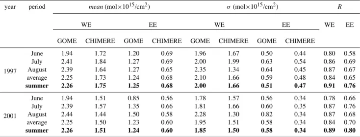
Table 2. Basic statistical characteristics of spatial distributions of GOME measurement derived and simulated tropospheric NO2columns for Western Europe (WE) and Eastern Europe (EE).
year period mean(mol×1015/cm2) σ(mol×1015/cm2) R
WE EE WE EE WE EE
GOME CHIMERE GOME CHIMERE GOME CHIMERE GOME CHIMERE
1997
June 1.94 1.72 1.20 0.69 1.96 1.67 0.50 0.44 0.80 0.58
July 2.41 1.84 1.27 0.69 2.00 1.99 0.63 0.54 0.86 0.69
August 2.39 1.64 1.27 0.65 2.35 1.34 0.64 0.45 0.87 0.67
average 2.25 1.73 1.24 0.68 2.10 1.66 0.59 0.48 0.84 0.65
summer 2.26 1.75 1.25 0.68 2.00 1.66 0.51 0.47 0.91 0.76
2001
June 1.94 1.51 0.85 0.56 1.78 1.57 0.56 0.34 0.78 0.66
July 2.39 1.57 1.35 0.66 1.81 1.66 0.60 0.35 0.87 0.76
August 2.44 1.44 1.50 0.58 2.28 1.30 0.82 0.34 0.87 0.68
average 2.25 1.50 1.23 0.60 1.95 1.51 0.58 0.34 0.84 0.70
summer 2.26 1.51 1.24 0.60 1.85 1.50 0.58 0.34 0.89 0.80
characteristics and a contribution of random errors, but also on systematic errors that covariate with the true values. For example, our situation with the larger standard deviations of GOME data than that of CHIMERE data could be explained by larger random errors (noise) in the data from GOME. But on the other hand, we could expect the similar result if the data from GOME or CHIMERE were scaled with a nearly constant factors that are less or greater than unity, respec-tively. Those factors would represent systematic multiplica-tive (geometric) errors of the respecmultiplica-tive data.
The potential sources of systematic errors in NO2columns
from a CTM and GOME are quite numerous and have al-ready been discussed in details by Savage et al. (2004) and Boersma et al. (2004). It is important that the most likely er-rors both in models and in the GOME retrieval procedure are indeed of a multiplicative character, as they are associated, on the one hand, with miscalculation of NO2 lifetime (due
to errors in vertical transport, chemistry and deposition) and, on the other hand, with uncertainties of the air mass factor (due, e.g. systematic errors in input vertical profiles of tropo-spheric NO2or scattering on aerosols).
Regarding the differences in statistics for Western and Eastern Europe, it is useful to note that while values of both the mean and the standard deviation are significantly smaller for Eastern Europe, the relative differences are much larger in the standard deviations than in the means. Consequently, the ratios of the standard deviation to the means of both GOME derived and simulated data for Western Europe are consider-ably larger than the corresponding ratios for Eastern Europe. Specifically, these ratios are 37% and 75% higher for West-ern than for EastWest-ern Europe in the case of CHIMERE data for 1997 and 2001, respectively. The differences are even much larger with the GOME data, because of more significant
con-Table 3.Statistical characteristics of upper tropospheric (below 500 hPa pressure level) NO2columns estimated using MOZART output database.
period mean(mol×1015/cm2) σ(mol×1015/cm2)
WE EE WE EE
June 0.48 0.57 0.07 0.06
July 0.51 0.56 0.10 0.08
August 0.55 0.55 0.14 0.09
average 0.51 0.56 0.10 0.08
summer 0.51 0.56 0.10 0.07
tribution of the free tropospheric NO2 to GOME data over
Eastern Europe. These results mean, in particular, that if val-ues of NO2columns for Eastern Europe were linearly scaled
to obtain the same means for the both regions, the variance of such scaled values for Eastern Europe would be considerably less than that of the data for Western Europe. This substan-tial difference in distributions of NO2columns over Western
6 Analysis of “random” (non-systematic) uncertainties of modelled and GOME measurement derived distri-butions of tropospheric NO2
6.1 Evaluation of the upper limit for the uncertainties Let us consider the following variance of the difference, E= 1
N XN
i=1
zig−zic− ¯zg+ ¯zc 2
, (3)
where zig and zic are values of NO2 columns derived from
GOME measurements and those simulated by CHIMERE for ani-th grid cell, respectively, whilez¯gandz¯care their mean values.
The meaning ofEbecomes easier to interpret if we write the following formal equalities,
zgi =zit +εgi +θg,
zci =zit+εci +θc, (4) wherezit is a true (unknown) value of tropospheric NO2
col-umn,εig andεic are random errors (with the zero means) of GOME derived and simulated NO2columns, and
θg,c = 1 N
XN i=1
zig,c−zit (5) are the systematic part of errors.
After substitution (4) into (3),Eis expressed as follows, E= 1
N XN
i=1
εig−εci2 (6) That is,Eis simply the mean squared difference of “random” (non-systematic) errors. If we assume further that these er-rors are almost independent, that is,
εgεc << ε2
g,c, (7)
then we find that E∼=ε2
g+εc2. (8)
So, under the given assumption,Erepresents the total mean squared error associated with both GOME derived and sim-ulated NO2columns. In other words, the evaluation ofE
al-lows us to estimate the upper limit of random component of the uncertainty of either of the two datasets considered. The assumption (7) seems to be very reasonable considering the principal differences in methods used to obtain the data that we compare. Even if a strong covariance existed between uncertainties of NO2columns simulated by CHIMERE and
MOZART, it could cause much smaller covariance between uncertainties of NO2columns simulated by CHIMERE and
those derived from GOME, because the latter are sensitive to vertical profiles of NO2rather than to their column amounts.
Possible reasons for a non-zero covariance between the un-certainties of CHIMERE and MOZART might be the use
of MOZART data for prescribing boundary conditions for CHIMERE and correlations of errors of anthropogenic emis-sions prescribed in the models. But it seems very unlikely that this covariance may be strong, taking into account that CHIMERE and MOZART use different chemical schemes, different gridded emission databases (EMEP and EDGAR, respectively), meteorological data, and, besides, have very different horizontal resolution.
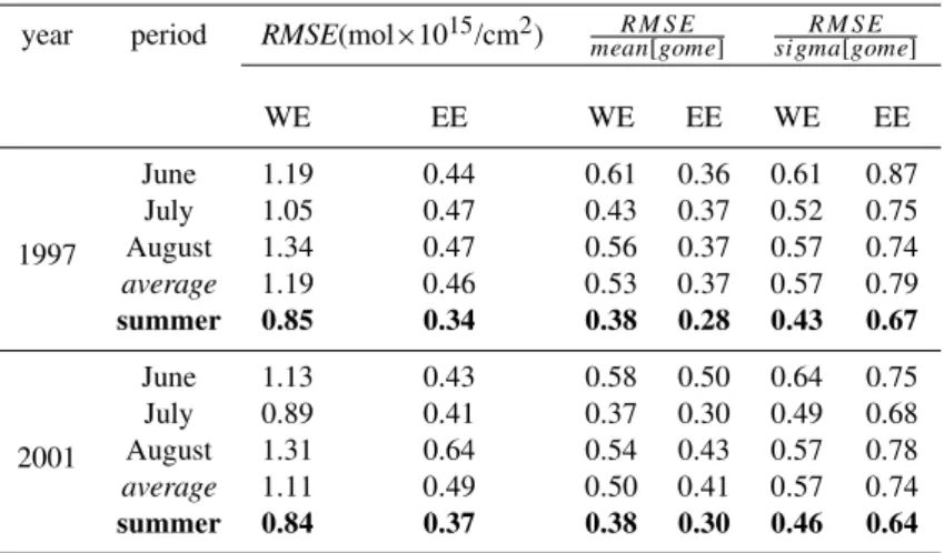
The squared roots ofE(that is, RMSE with respect to ran-dom errors) and their normalized values are listed in Table 4. It is seen that the errors are rather significant for both regions, and that they are larger when compared with the standard de-viations than with the means of GOME derived data, espe-cially for Eastern Europe. The ratio of RMSE to the stan-dard deviation (it is sometimes referred to as the root relative squared error) characterizes, in our case, uncertainties in spa-tial variability of NO2columns. The uncertainties of the data
averaged over three months are less than the uncertainties of the monthly datasets, but it is easy to see that their reductions are smaller than it could be expected if the errors for different months were independent (that is, the reductions are smaller than the square root of 3). Hence, we can conclude that a significant part of the error is persistent beyond the monthly time scale.
It is noteworthy that while the ratios of RMSE to the mean are larger for Western Europe, the ratios of RMSE to the stan-dard deviation are much larger for Eastern Europe. There-fore, based on these results it seems impossible to conclude unambiguously whether the agreement between simulated and GOME derived data is better for one or the other part of Europe. The reason has already been discussed in the pre-vious section. Nevertheless, as it is shown below, the picture will become clearer when analysing uncertainties as a func-tion of magnitudes of the NO2columns.
6.2 The random error as a function of amplitude of NO2
columns
As a preliminary step to further analysis, we would like to introduce the following simplified model of errors. Let us as-sume that values of tropospheric NO2columns derived from
GOME measurements,zg, relate to their true values,zt, as follows:
zg=zt(1+δs,g+δr,g)+1s,g+1r,g, (9) where δs,g,δr,g,1s,g and1r,g are systematic and random parts of multiplicative and additive errors, respectively. It is assumed thatδs,g and1s,g are constants, whileδr,g and 1r,gare random variables independent ofztand having zero means. Such assumptions are hardly satisfied exactly in any real situation, but they still may be a reasonable and useful approximation. The same kind of an error model is used be-low for NO2columns from CHIMERE, after the replacement
Table 4. Statistics for the total random errors of tropospheric NO2columns derived from GOME measurements and those calculated by CHIMERE.
year period RMSE(mol×1015/cm2) meanRMSE[gome] sigmaRMSE[gome]
WE EE WE EE WE EE
1997
June 1.19 0.44 0.61 0.36 0.61 0.87
July 1.05 0.47 0.43 0.37 0.52 0.75
August 1.34 0.47 0.56 0.37 0.57 0.74
average 1.19 0.46 0.53 0.37 0.57 0.79
summer 0.85 0.34 0.38 0.28 0.43 0.67
2001
June 1.13 0.43 0.58 0.50 0.64 0.75
July 0.89 0.41 0.37 0.30 0.49 0.68
August 1.31 0.64 0.54 0.43 0.57 0.78
average 1.11 0.49 0.50 0.41 0.57 0.74
summer 0.84 0.37 0.38 0.30 0.46 0.64
model to our data in order to try to estimate their multiplica-tive and absolute errors independently.
The idea of the following analysis is to obtain informa-tion on the additive and multiplicative parts of the error, by repeating error analysis in a similar way as in the previous section, but separately for subsets of data with similar mag-nitudes. More specifically, we will have to evaluate the vari-anceE given in (3) for each of the subsets. The selection of the subsets is based on the procedure of a “running win-dow” applied to data preliminary arranged with growing am-plitude.
Let us consider which kind of information we can get from such a procedure. For definiteness, we consider a case when the selection procedure is applied to GOME data, but same reasoning also holds for CHIMERE data. In such a case, a “local” version of the variance (3) after substitution ofzgand zcfrom (9) takes the form:
Eg = 1 Nw
XNw
j=1
(zi(j )t − ¯zt)(δs,g−δs,c)+zti(j )(δ i(j )
r,g −δi(j )r,c )−ztδr,g+1i(j )r,g −1i(j )r,c 2
,
(10)
where Nw is the number of datapoints in the window, and the averaging is performed over the set of the selected data. Let us assume that the total ensemble of the data is suffi-ciently large, so that the variance of the GOME data within the “window“ can be neglected when compared to their er-rors. Assume also that typical scales of all systematic and random multiplicative errors are much less than unity. Then, after substitution ofztfrom (9) to (10) and having performed Taylor’s expansion ofEgup to quadratic terms with respect
to allδs andδr, we obtain the following:
Eg≈
δ2 r,g+δ2r,c
1+δs,g2
zg−1s,g 2
+12
r,g+12r,c
+(δ
2
r,g+δr,c2 ) (1+δs,g)21
2 r,g−
2(δs,g−δs,c) (1+δs,g) 1
2
r,g (11)
It is easy to see that if the approximation (11) is valid and the magnitudes ofzg are sufficiently large, we should expect a quasi-linear growth of (Eg)1/2with the increase ofzg. The squared rate of such a growth can give an estimate of the upper limit of the random part of the mean squared relative error (MSRE) associated with multiplicative errors. Indeed, by definition we have:
MSREg = z
g−zt zg
2
. (12)
Using (9), assuming thatzt(δs+δr)≫1s,1r, and performing Taylor’s expansion of the denominator, we find that
MSREg ≈ δ2r,g
(1+δs,g)2 + δ2s,g
(1+δs,g)2. (13)
The first term in the right hand side of (13), which corre-sponds to the random part of the multiplicative errors, is al-ways less or equal to the rate of growth ofEgdetermined by the fraction in the first term on the right-hand side of Eq. (11). For convenience, we report below our estimations in terms of the squared root of the random part of MSRE, that is RM-SRE.
It follows also from (11) that for the limiting case of zg near zero, the evaluations ofEallow us to estimate the upper limit for random additive errors. Indeed, it is easy to see that 12
Fig. 7.Running averages of squared differences between the deviations of the simulated and GOME measurement derived tropospheric NO2 columns from their running mean values versus the running averages of the indicated data for Western Europe. The averaging procedure using a running window covering 100 data points is applied to the gridded data for the seasonally averaged tropospheric NO2columns from GOME or CHIMERE (as indicated in the figures) arranged with growing amplitude. The points on the curves are depicted with a frequency of 1/100.
Figure 7 presents the dependences of the “running” evalua-tions ofE1/2, as a function of the corresponding running av-erages of the GOME or CHIMERE NO2columns for
West-ern Europe. The running averages and statistics were cal-culated using a window consisting of 100 consecutive data points after the arrangement of all pixels in a growing order (with respect of GOME derived or simulated NO2columns.)
Such a window was chosen as a reasonable compromise be-tween poorer statistics and higher resolution that could be ob-tained with a narrower window and richer statistics but lower resolution with a wider window. We have found, however, that even the use of very different windows (covering, for ex-ample, 50 or 200 points) would not lead to serious changes in our results.
It is seen that along with random fluctuations, there is a well-pronounced quasi-linear positive trend in magnitudes of uncertainties. The largest deviation from the linear law takes place for the biggest NO2columns in the case of the
depen-dencies on the running averages of CHIMERE data. This exception concerns, however, only a small part (less than 8 %) of the total number of data points. In accordance to (11), these trends are indicative of predominant role of mul-tiplicative errors in total uncertainties of both GOME and CHIMERE data. As argued above, the root of the random part of the mean squared relative (multiplicative) errors can be estimated using the slopes of the linear fits of dependence ofE1/2on the magnitude of respective data. It is noteworthy that the slopes of the best linear fits are significantly different in the cases of CHIMERE and GOME data. The difference in the slopes can be caused by difference in the systematic errorsδs,gandδs,c(see Eq. 11).
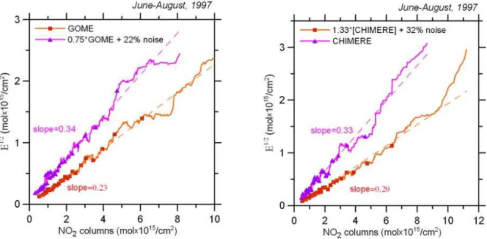
In order to get an idea of possible uncertainties of our procedure, we have performed a special numerical
exper-iment using the data for 1997 as example. Specifically, we have preliminarily defined two pairs of the datasets, the first of which includes the original and specially transformed datasets for NO2columns from GOME, and the second one
includes the original and specially transformed datasets for NO2columns from CHIMERE. The transformations are
per-formed by adding artificial systematic and random multi-plicative errors to the original data. The idea is to estimate a priori known errors using the procedure described above. The artificial errors have been prescribed based on the eval-uations of real errors of the original data. Specifically, in the case with GOME data, we have applied a systematic error δs=−0.25, based on the value of a slope (0.75) of the corre-sponding best linear fit in Fig. 6, and random multiplicative errorsδr with the standard deviation of σr=0.22, in accor-dance to the slope of the corresponding fit in Fig. 7. Such transformed data were used as a substitute for the CHIMERE data. Similarly, in the case with the CHIMERE data, we have prescribed δs=0.33 (0.75−1-1) and σr=0.32 and used such transformed data as a substitute for the GOME data. The random errors have been sampled from the lognormal distri-bution. Afterwards, we have applied our “running window” analysis to each of the two pairs datasets independently. The results of the analysis of such artificial errors are presented in Fig. 8.
Fig. 8.The interpretation of the results presented in Fig. 7. The plots show the results of the same error analysis as in Fig. 7, but aimed at retrieving the known “errors” of the artificially transformed dataset. The “running window” analysis was applied to two pairs of the original and transformed datasets indicated in the figures, and the “running” RMSEs are plotted against the running averages of the indicated data.
can expect that our estimations of the upper limit of multi-plicative errors of the real data for Western Europe may be uncertain within about 20%. However, taking into account that both CHIMERE and GOME data are not quite perfect and that their partial errors are therefore significantly smaller than the total errors, it seems to be indeed safe to conclude that the random part of the mean squared relative error of NO2columns from CHIMERE and GOME for Western
Eu-rope is, on the average, less than 32 and 23 percent, respec-tively. The contribution of the additive errors is not well pro-nounced, but it is evident that they are, on the average, less than 3×10¹⁴mol/cm2(see Eq. 14 and Fig. 7).
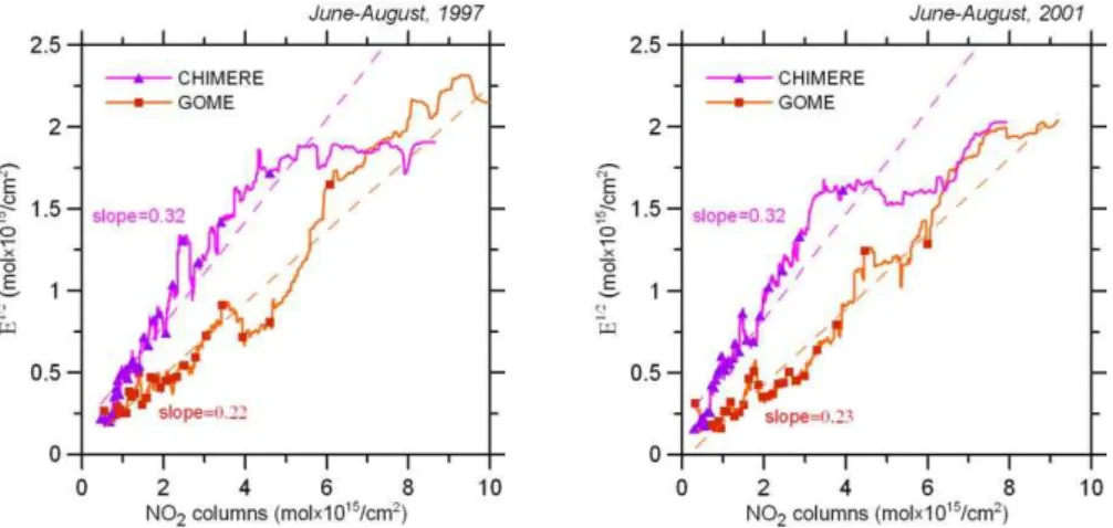
Figure 9 presents the results of similar analysis for Eastern Europe. In order to facilitate a comparison between the re-sults for Western and Eastern Europe, this figure reproduces also the corresponding section of the curves for Western Eu-rope. The most surprising result is that the uncertainties for Eastern Europe are substantially lower than the uncertainties for Western Europe for the major part of the range of magni-tudes of NO2columns for Eastern Europe, especially when
the uncertainties are considered versus the data from GOME. Indeed, it seemed to be reasonable to expect that the poten-tial uncertainties of input information used in CHIMERE and for retrieval of GOME NO2 columns are larger for Eastern
Europe than for Western Europe. Probably, this result is, mainly, due to the fact that Western European regions with relatively low levels of NO2pollution are usually situated in
the vicinity of much more polluted regions, whereas for East-ern Europe they are more homogeneous and wide spread. As a consequence, the uncertainties of the NO2transport
simu-lated by CHIMERE, on the one hand, and a low resolution of MOZART data used to evaluate AMF, on the other hand, may play much more significant role under considered con-ditions in Western Europe than in Eastern Europe.
It is evident that the uncertainties for Eastern Europe have more complex character than those for Western Europe with a less clear correlation between uncertainties and absolute NO2 columns. However, they also demonstrate positive
trends with the increase of the magnitudes of NO2columns,
which are indicative of multiplicative errors. The estimates for multiplicative and additive errors can be obtained in the same way as in the case of Western Europe. However, the considerable scattering of the fitted uncertainties indicates that the error model (9) is less relevant in this case, and the error estimates are much less accurate than those in the case of Western Europe. Note also that because of significant con-tribution of additive errors, the slopes of the fits for E1/2 given in Fig. 9 may underestimate actual values of the root of the random part of MSRE. Therefore, any error estimates for Eastern Europe that can be obtained using results presented in Fig. 9 should be used with much care.
The analysis with a running window has been repeated for each of the summer months of 1997 and 2001, and corre-sponding estimations of the relative errors are listed in Ta-ble 5. As it could be expected, the errors of the monthly mean data are, on the average, larger than the errors of the seasonally averaged datasets. The monthly estimates are rather divergent, but have some common features in different years. For example, the difference between the estimates for CHIMERE and GOME data are largest for Western and East-ern Europe in August of both 1997 and 2001. This and some other similarities between our results for 1997 and 2001 may be due to some regular differences in quality of the data from CHIMERE and GOME in different months of a year. 6.3 Discussion
tropo-Fig. 9.The same as in Fig. 7, but for Eastern Europe. For convenience, the plots reproduce also a subsection of the dependences for Western Europe.
Table 5.Estimations of the upper limits of the mean random relative (multiplicative) error (%) of tropospheric NO2columns retrieved from GOME measurements and those calculated by CHIMERE.
year period WE EE
GOME CHIMERE GOME CHIMERE
1997
June 33 49 14 30
July 36 29 26 28
August 17 59 19 37
average 29 46 20 32
summer 22 32 15 24
2001
June 31 39 10 14
July 26 30 7 21
August 16 52 7 41
average 24 40 11 25
summer 23 32 6 24
spheric NO2columns derived from GOME measurement and
those simulated by the models. As pointed out before, the multiplicative and additive errors defined above represent up-per limits of random errors both in the GOME derived and simulated NO2column.
The main sources of errors in the GOME NO2 columns
are (i) the fit of NO2 column from the spectrum, (ii)
sepa-ration of stratospheric and tropospheric NO2, and (iii)
eval-uation of tropospheric light path (including uncertainties as-sociated with the surface albedo, AMFs, and cloud effects). For the Bremen V1 dataset, Richter and Burrows (2002) es-timated the random (both in time and space) uncertainties associated with each individual NO2 fit to be in the range