A review of the ozone hole from 2008 to 2010 as observed by IASI

(1)

AMTD

4, 4717–4752, 2011

A review of the ozone hole from 2008 to 2010 as observed by

IASI

C. Scannell et al.

Title Page Abstract Introduction Conclusions References Tables Figures

◭ ◮

Back Close Full Screen / Esc

Printer-friendly Version Interactive Discussion

Discussion

P

a

per

|

Dis

cussion

P

a

per

|

Discussion

P

a

per

|

Discussio

n

P

a

per

|

Atmos. Meas. Tech. Discuss., 4, 4717–4752, 2011 www.atmos-meas-tech-discuss.net/4/4717/2011/ doi:10.5194/amtd-4-4717-2011

Atmospheric Measurement Techniques Discussions

This discussion paper is/has been under review for the journal Atmospheric Measure-ment Techniques (AMT). Please refer to the corresponding final paper in AMT

if available.

A review of the ozone hole from 2008

to 2010 as observed by IASI

C. Scannell1, D. Hurtmans2, A. Boynard1,*, J. Hadji-Lazaro1, M. George1, A. Delcloo3, O. Tuinder4, P.-F. Coheur2, and C. Clerbaux1,2

1

UPMC Univ. Paris 06, CNRS/INSU, UMR8190, LATMOS-IPSL – Universit ´e Versailles St.-Quentin, Paris, France

2

Spectroscopie de l’Atmosph `ere, Chimie Quantique et Photophysique, Universit ´e Libre de Bruxelles (ULB), Brussels, Belgium

3

Royal Meteorological Institute of Belgium, Uccle, Belgium

4

oyal Netherlands Meteorological Institute, De Bilt, The Netherlands

*

now at: Atmospheric Chemistry Division, National Center for Atmospheric Research, Boulder, CO, USA

Received: 23 May 2011 – Accepted: 7 July 2011 – Published: 22 July 2011 Correspondence to: C. Scannell (claire.scannell@gmail.com)

(2)

AMTD

4, 4717–4752, 2011

IASI

C. Scannell et al.

◭ ◮

Discussion

P

a

per

|

Dis

cussion

P

a

per

|

Discussion

P

a

per

|

Discussio

n

P

a

per

|

Abstract

Atmospheric remote sensing from satellites is essential for the long-term, continu-ous monitoring of the ozone hole and is critical in order to evaluate stratospheric ozone recovery. During the last decade, thermal infra-red (TIR) sensors have demon-strated their enhanced capability in capturing both the spatial and temporal variability 5

of the ozone hole during the polar night, in contrast to instruments measuring in the ultraviolet-visible (UV-vis) range of the spectrum which need sunlight to operate. In this paper we present a study of the ozone hole as observed by the Infra-red Atmospheric Sounding Interferometer (IASI) on-board the MetOp-A European satellite platform from the beginning of data dissemination, August 2008, to the end of December 2010. Here 10

we demonstrate IASI’s ability to capture the seasonal characteristics of the ozone hole. We compare IASI ozone total columns and vertical profiles with those of the Global Ozone Monitoring Experiment 2 (GOME-2) (also on-board MetOp-A) and electrochem-ical concentration cell (ECC) ozone sonde measurements for the ozone hole region and period. The IASI and GOME-2 ozone total columns were found to be in excellent 15

agreement for this region with a correlation coefficient of 0.97, for September, October and November 2009. IASI on average, exhibits a positive bias of approximately 7 % compared to the GOME-2 measurements over the entire ozone hole period. Compar-isons between IASI and ozone sonde measurements were also found to be in good agreement with the percentage di_fference between both ozone profile measurements 20

(3)

AMTD

4, 4717–4752, 2011

IASI

C. Scannell et al.

◭ ◮

Discussion

P

a

per

|

Dis

cussion

P

a

per

|

Discussion

P

a

per

|

Discussio

n

P

a

per

|

1 Introduction

Global monitoring of ozone (O₃) is essential as it plays an important role in the chemical processes occurring in the atmosphere and has a major impact on the climate. In the troposphere ozone is considered to be one of the primary air pollutants and main greenhouse gases and in high pollution areas it has been shown to have significant 5

negative impacts on human health and local ecosystems (Slaper et al., 1996). In the stratosphere however, where ozone concentrations greatly exceed those of the troposphere, ozone works to protect the Earth by absorbing the sun’s harmful ultraviolet (UV) radiation.

Since the mid 1980s a noticeable severe depletion of stratospheric ozone (reducing 10

to less than 100 DU (₌Dobson Units) compared to the average stratospheric ozone concentration of∼300 DU outside of the ozone hole period) has been observed annu-ally over the Antarctic region during the polar springtime (August, September, October and November). Studies into the distribution and evolution of this ozone hole have es-tablished that during this period the ozone hole extends over the Antarctic region and 15

increases the level of UV radiation reaching the Earth’s surface in the ozone hole re-gion (Newman et al., 2007). This in turn leads to adverse impacts on human health in parts of Australia and South America due to their close proximity to the Antarctic ozone hole (de Laat et al., 2010; Slaper et al., 1996).

Ozone loss rates are determined by the concentrations of active chlorine, bromine, 20

nitrogen and hydrogen oxides present in the atmosphere. It is thought that approxi-mately 60 % of the ozone destruction is caused by the release of active chlorine and the remainder by the release of bromine, hydrogen and nitrogen (Feng et al., 2005). During the polar night (the period in which the Antarctic is in darkness), a polar vor-tex forms in the Antarctic, holding the air mass within. The lack of sunlight leads to 25

(4)

AMTD

4, 4717–4752, 2011

IASI

C. Scannell et al.

◭ ◮

Discussion

P

a

per

|

Dis

cussion

P

a

per

|

Discussion

P

a

per

|

Discussio

n

P

a

per

|

take place on the surface of PSCs resulting in the release of active chlorine which is a key element in the catalytic destruction of ozone over the Antarctic when the sun comes back. Furthermore nitric acid (HNO₃), a by-product of the heterogeneous reac-tions remains within the PSCs, which are lost from the stratosphere via sedimentation. This denitrification process results in the unavailability of NO_x to sequester the active 5

chlorine species.

The Montreal protocol and its amendments were designed to protect the ozone layer by phasing out the production of ozone depleting substances containing chlorine and bromine. At the most recent scientific evaluation of the effects of the treaty it was demonstrated that there is evidence of a decrease in the atmospheric burden of ozone 10

depleting substances and that there are some signs of early stratospheric ozone re-covery (WMO, 2010). Thus the monitoring of the Antarctic ozone is critical in order to evaluate the effectiveness of this treaty.

Long-term change and variability in ozone levels in the Antarctic have been recorded from several ground based monitoring stations since the discovery of the ozone hole in 15

the 1980s (Fortuin and Kelder, 1998; Balis et al., 2003). These in-situ measurements however are limited both in time and space and though they provide a clear picture of ozone profiles in the Antarctic they fail to o_ffer a complete picture of the temporal and spatial evolution of the ozone hole. Satellite measurements can complement these existing in-situ measurements by providing a unique perspective from which to view 20

the ozone hole, having the capability of providing daily, long term measurements. Cur-rent ozone depletion monitoring relies on UV-vis instruments onboard satellites such as TOMS (Total Ozone Mapping Spectrometer), GOME (Global Ozone Monitoring Ex-periment) and OMI (Ozone Monitoring Instrument), (McPeters and Labow, 1996; Van Roozendael et al., 2006; Liu et al., 2010). Such instruments while revolutionizing the 25

(5)

AMTD

4, 4717–4752, 2011

IASI

C. Scannell et al.

◭ ◮

Discussion

P

a

per

|

Dis

cussion

P

a

per

|

Discussion

P

a

per

|

Discussio

n

P

a

per

|

a result these instruments have large data gaps which can be filled using assimilated data.

The advent of thermal infrared (TIR) sounders such as IASI (Infrared Atmospheric Sounding Interferometer) onboard MetOp-A complements the available datasets, with the advantage that both day and night time measurements are available at high spa-5

tial resolution with a small footprint. Here we present a comprehensive study of the ozone hole as viewed by IASI since the beginning of its operation and data dissem-ination (2008, 2009 and 2010). After a description of the instrument characteristics and the retrieval process (Sect. 2), a detailed description of the Antarctic ozone hole as observed by IASI is provided (Sect. 3). In Sects. 4 and 5 we then evaluate the 10

IASI ozone total column and profile observations along with GOME-2 (which is also onboard the MetOp-A satellite platform) data and in-situ measurements from ground based stations.

2 Ozone retrievals from IASI spectra

2.1 The IASI instrument

15

The IASI instrument is a high resolution, nadir viewing Fourier transform spectrometer measuring in the thermal infrared part of the spectrum, between 645 and 2760 cm−1_. It was launched on board the sun synchronous polar orbiting MetOp-A satellite pla×2 circular pixels each with a ground footprint of 12 km at the nadir and it has an across track scan with a swath width of 2200 km. It is characterized by a spectral resolution of 20

0.5 cm−1 (apodized) and a spectral sampling of 0.25 cm−1. Depending on the surface temperature and spectral range the retrieved spectra have low radiometric noise esti-mated to be within the 0.1–0.4 K and around 0.2 K in the ozone 10 µm region. Due to its large spatial coverage, combined with its low radiometric noise IASI provides twice daily global measurements of key atmospheric species enabling the analysis of species 25

(6)

AMTD

4, 4717–4752, 2011

IASI

C. Scannell et al.

◭ ◮

Discussion

P

a

per

|

Dis

cussion

P

a

per

|

Discussion

P

a

per

|

Discussio

n

P

a

per

|

HNO₃(Wespes et al., 2009). Other reactive species which are retrieved include carbon monoxide (CO) (George et al., 2009; Pommier et al., 2010), methane (CH₄) (Razavi et al., 2009), sulphur dioxide (SO₂) (Clarisse et al., 2008), ammonia (NH₃) (Clarisse et al., 2009), methanol (CH₃OH) and formic acid (HCOOH) (Coheur et al., 2009; Razavi et al., 2010). For a full detailed overview of the IASI instrument, its specifications and 5

trace gas species that can be retrieved (see Clerbaux et al., 2009).

The IASI mission delivers approximately 1.3×106 spectra per day, which are dis-seminated via Eumetcast, the EUMETSAT data distribution system, 3 h after observa-tion. The absorption lines contained within each spectra are related to the trace gas concentrations via a non linear function of characteristics at the point of measurement 10

such as surface emissivity, temperature profile, other atmospheric components which may interfere with the signal (other trace gases, clouds, aerosols, etc.) and also the characteristics of the instrument itself (spectral resolution, footprint, radiometric noise). To retrieve information about specific atmospheric trace gases from these spectra an inversion algorithm/retrieval scheme needs to be applied.

15

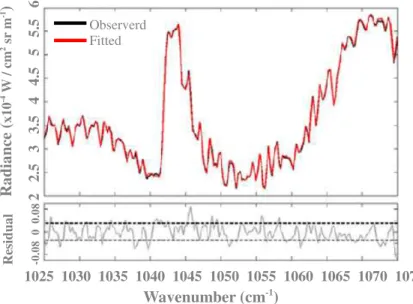
Figure 1 shows part of the intense (high absorbing) ozone band around 9.6 µm used for retrievals. The black and red spectra represent the observed and fitted IASI spectra respectively. Both spectra clearly portray the characteristic lines in the spectrum asso-ciated with ozone absorption in this spectral window (960–1075 cm−1). The grey line shows the residual of the fit which is the di_fference between what is observed and what 20

is fitted, compared to the instrument noise level (dashed line) in this spectral range. From these spectra we retrieve both columns (total and partial) and profiles from 0– 40 km in altitude. Retrievals are performed for scenes with cloud coverage of less than 13 %, using the EUMESAT operational level 2 cloud coverage information, temperature and humidity profiles.

25

2.2 IASI ozone retrievals

(7)

AMTD

4, 4717–4752, 2011

IASI

C. Scannell et al.

◭ ◮

Discussion

P

a

per

|

Dis

cussion

P

a

per

|

Discussion

P

a

per

|

Discussio

n

P

a

per

|

observations per day which are disseminated via the Eumetcast antenna system. In a previous study (Boynard et al., 2009), systematic retrievals of ozone total columns were performed using an algorithm based on the Neural Network (NN) technique (Tur-quety et al., 2004). For the early stage IASI processing only measurements with a scan angle below 32◦ _{on either side of the nadir was considered, and specific issues}

5

were identified over icy and sandy surfaces due to the di_fficulty to properly train the net-work with insufficient knowledge of the actual emissivity. This while providing a good global overview of the distributions and concentrations of ozone, made it difficult to focus on particular locations such as the Antarctic as not only were there large gaps between each overpass due to the narrow scan angle but also data gaps at the poles, 10

particularly in the southern hemisphere. The Boynard et al. (2009) study found that in general IASI ozone total columns were in good agreement with both GOME-2 and with the Brewer and Dobson ground based instruments with correlation coefficients of 0.9 and 0.85 respectively. This study also found that IASI had a positive bias of about 3.3 % when compared to both GOME-2 and the ozone sondes measurements.

15

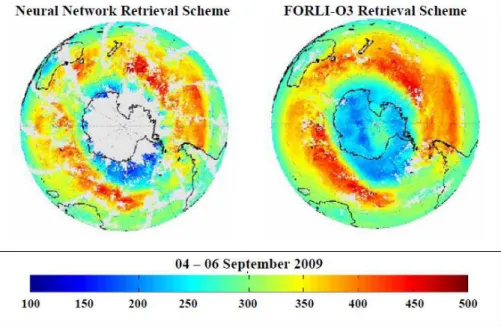
In order to allow the processing of more IASI data at any location the FORLI (Fast Optimal Retrievals on Layers for IASI) O₃ retrieval code was developed at the Uni-versit ´e Libre de Bruxelles (ULB) to continuously retrieve ozone profiles from the IASI radiance spectra. Figure 2 shows an Antarctic projection of ozone total column distri-butions averaged over 3 days at the peak of the 2009 ozone hole (4–6 September), 20

retrieved from the NN scheme and from the FORLI-O3 scheme. It clearly highlights the improved capability of IASI to capture the spatial variability of total ozone columns in the Antarctic region when using the FORLI-O3 scheme. The FORLI scheme unlike the initially developed NN scheme has no limit on scan angle width and can adjust the surface temperature and thus processes all the data resulting in a much greater spatial 25

coverage.

(8)

AMTD

4, 4717–4752, 2011

IASI

C. Scannell et al.

◭ ◮

Discussion

P

a

per

|

Dis

cussion

P

a

per

|

Discussion

P

a

per

|

Discussio

n

P

a

per

|

minimize the computational time necessary for the retrieval of such a huge quantity of data. These tables are pre-computed on a logarithmic grid for pressure (4.5x10−5 _–

1atm) and on a linear grid for temperature (162.8 K–322.64 K) and relative humidity for the water vapour table, using the HITRAN databases (Rothman et al., 2005 and 2009). The Level 2 temperature data distributed by the Eumetcast system are used as input 5

of the code as well as surface emissivity from the MODIS/TERRA or IASI climatology depending on the version of FORLI which is used (Wan, 2008).

The inverse (retrieval) scheme is based on the Optimal Estimation Method (OEM) (Rodgers, 2000) and was developed for the retrieval of ozone profiles from high resolu-tion nadir infrared radiances (e.g. Coheur et al., 2005). This method gives the optimal 10

solution for a state vectorx(in this case the O3profile), for given a measurementy, the IASI radiance spectra, with an error covarianceS_ε and the equationy₌F(x, b)+ε, whereF is the forward radiative transfer model, b represents the model parameters a_ffecting the measurement andεis the measurement noise.

Solving such a problem is complex as there can be many solutions which fit the 15

observations. Therefore to find a meaningful solution it is necessary to constrain the results with some a priori information,x_athe a priori profile that represents the expected average profile andS_athe covariance matrix that ideally represents the true variability of the species about the average. The solution can be found by iteratively applying:

ˆ

xi+1 = xa + Dy

y ₋ F ( ˆxi) − Ki xa − xˆi

(1) 20

withDy=SˆiKiTS

−1

ε and ˆSi+1=(KiT+1S− 1

ε Ki+1+S−a1)−1 whereKi=(∂F_∂x)i is the Jacobian at statex_i,K_iT is its transpose and ˆxi+1 is the new state vector. The matrixDy is the matrix of contribution factors and the error covariance of the solution is given by ˆS_i₌₁. The iteration starts with some initial estimate of the state, the a priori informationx_a, and the covariance matrixS_a, and terminates when convergence is reached.

25

(9)

AMTD

4, 4717–4752, 2011

IASI

C. Scannell et al.

◭ ◮

Discussion

P

a

per

|

Dis

cussion

P

a

per

|

Discussion

P

a

per

|

Discussio

n

P

a

per

|

2007). This ozone climatology is altitude dependent and consists of monthly averaged ozone profiles for 10◦_{latitude zones from 0 to 60 km. This climatology is a combination}

of data from the Stratospheric Aerosol and Gas Experiment II (SAGE II; 1988–2001), the Microwave Limb Sounder (MLS; 1991–1999) and data from balloon sondes (1988– 2002). Such a global climatology aids in the construction of a priori information as it 5

represents a good approximation of the average state of the atmosphere.

To allow for a useful comparison with other data sets, a smoothing of the true retrieval state is necessary and is characterized as follows by Eq. (2).

ˆ

x ₌ Ax ₊ (I − A)xa (2)

where ˆx is the retrieved profile, Ais the averaging kernel matrix, x is the true profile 10

andx_ais the a priori profile. The averaging kernels indicate the measure of sensitivity of the retrieved state ˆx to the true state x. The trace ofA, representing the degrees of freedom for the signal (DOFs), measures the number of independent pieces of in-formation available from the retrieval and gives an estimation of the vertical sensitivity of the retrievals. FORLI-O3 generates ozone partial columns in 40, 1 km thick layers, 15

along with the associated averaging kernels and errors matrices. Using FORLI-O3 the complete structure of the ozone hole along with ozone concentrations are clearly discernible and the full extent of the vortex is captured.

3 The Antarctic ozone hole as seen by IASI

Figure 3 shows two IASI infrared spectra taken over the Antarctic in September 2009 20

and the ozone band for each spectrum is highlighted by the circled areas. The blue spectrum is representative of spectra over the ocean close to main land Antarctica and the red spectrum is representative of those taken over the Antarctic continent itself (both measurements are located in Fig. 4, marked a and b respectively). Over the ocean the retrieved spectrum shows the ozone band absorption in the thermal infrared 25

(10)

AMTD

4, 4717–4752, 2011

IASI

C. Scannell et al.

◭ ◮

Discussion

P

a

per

|

Dis

cussion

P

a

per

|

Discussion

P

a

per

|

Discussio

n

P

a

per

|

is observed, it is weaker and the absorption lines seem to disappear due to the com-bined absorption and emission in the atmospheric layers (due to specific temperature conditions).

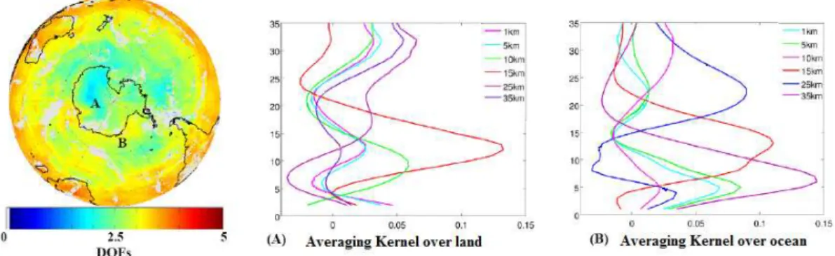
A global distribution of the DOFs and the averaging kernels associated with each of these spectra are depicted in Fig. 4. This figure highlights the difficulties in retrieving 5

ozone concentrations over the Antarctic region. As previously discussed, the DOFs are a measure of the vertical sensitivity of the measurement, i.e. the higher the number of DOFs the more vertical layers can be discriminate. Figure 4 (left panel) shows that over the ocean, the DOFs generally range between 3 and 4, while over the ice caps the DOFs range between 1 and 2. Because of the weaker signal over the ice, part of 10

the vertical information is lost. These results indicate that care is needed when select-ing spectra over the Antarctic land mass. As shown in Fig. 4 (middle), the averagselect-ing kernels associated with the measurement over the ocean are well defined, with DOFs of 3.3, while those associated with the measurement taken over the ice (Fig. 4, right panel) can appear ill formed, with DOFs of less than 1.5.

15

The ozone hole area is defined as the region of ozone located south of 40◦S and where ozone values fall below the threshold value of 220 DU (WMO, 2002). Recent studies have shown that during the 1980s the ozone hole over Antarctica expanded rapidly, this expansion slowed in the 1990s and in the last few years this expansion and ozone loss rates have appeared to level out but also the ozone loss rates (Newman et 20

al., 2006, 2009).

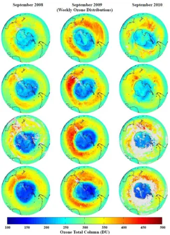
Figure 5 shows an example of typical ozone maps over the Antarctic during the ozone hole period. The maps plot the weekly averaged IASI ozone total columns on a 1◦

×1◦ grid for the September of 2008, 2009 and 2010. This period marks the time when the ozone hole area is at its largest and when ozone loss for this region is at its 25

greatest. Such distribution maps show that the size, shape and evolution of both the hole, its vortex and the ozone concentrations of both can be clearly monitored.

(11)

AMTD

4, 4717–4752, 2011

IASI

C. Scannell et al.

◭ ◮

Discussion

P

a

per

|

Dis

cussion

P

a

per

|

Discussion

P

a

per

|

Discussio

n

P

a

per

|

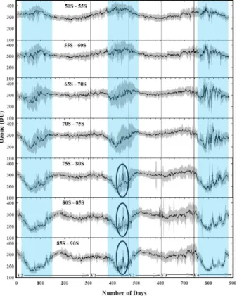
from 50◦_{S to 90}◦_{S, from the beginning of August 2008 to the end of December. It is}

worth noting here that FORLI-O3 algorithm has been upgraded several times since its development and as such this data set was obtained using slightly different versions of the algorithm. The shaded grey area represents the standard deviation (±σ) about this average. Apart from a few spurious points, the spread of the data is minimal for all 5

periods outside the ozone hole phase. The highlighted blue area represents the ozone hole period, August to December of each year. This figure clearly illustrates the sea-sonal cycle of ozone reduction over the Antarctic during the polar spring, beginning at the end of August and finishing by the end of November. For all years distinct features exist. One such feature is that the ozone hole itself forms annually south of 60◦_S.

An-10

other is that north of 60◦_{S there is a noticeable rise in ozone concentrations during the}

ozone hole periods which are representative of the edge of the vortex surrounding the ozone hole. Moving southwards it is also evident that the decrease in ozone concen-trations and the longevity of the hole itself become more pronounced. Each year the peak of the ozone hole occurs by mid September and at this time ozone concentrations 15

are seen to decrease by more than 50 % below 75◦_{S to approximately 150 DU.}

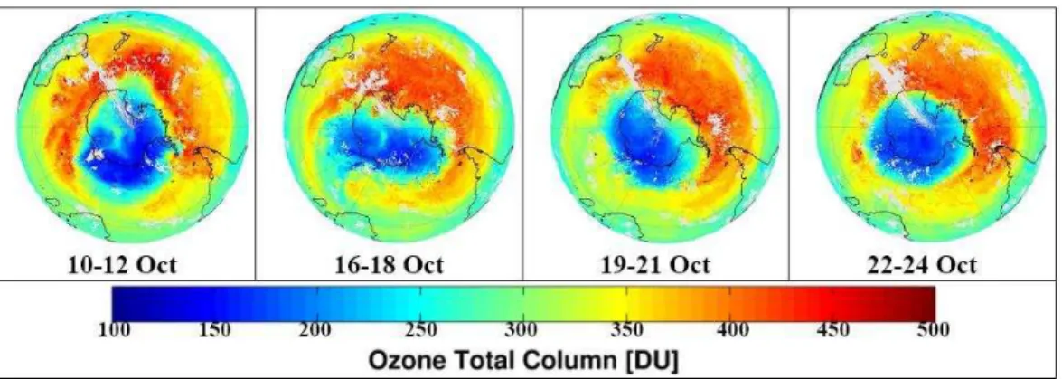
Despite these well observed trends there are some inter-annual variations. In 2009 there was a sharp increase in ozone concentrations in mid October (circled areas) that is not visible in 2008 or 2010. Figure 7 illustrates how during this period the polar vortex became more elliptical in shape. This lead to the early depletion of polar stratospheric 20

clouds in some regions that were previously within the vortex, as they became exposed to sunlight resulting in the increase in ozone concentrations (British Antarctic Survey, 2010). By 22 October the polar vortex had reverted back to the more standard circular rotation reducing ozone concentrations within the hole to levels similar to those prior to its elliptical circulation. In 2010 there was a relatively slow start to the ozone hole 25

(12)

AMTD

4, 4717–4752, 2011

IASI

C. Scannell et al.

◭ ◮

Discussion

P

a

per

|

Dis

cussion

P

a

per

|

Discussion

P

a

per

|

Discussio

n

P

a

per

|

period extended into late December with ozone values not rising above the 220 DU threshold limit until 21 December. For this 3 year study the ozone hole area was at its largest for this time of the year.

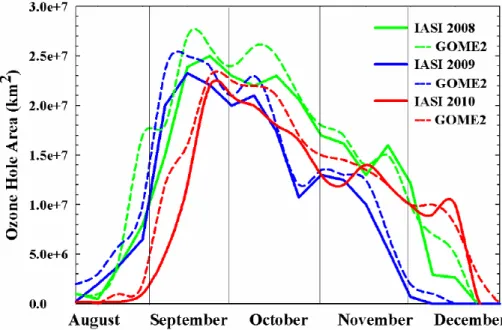
Figure 8 (solid lines) illustrates the temporal evolution of the ozone hole area from August to the end of December for 2008 (green), 2009 (blue) and 2010 (red). It is 5

compiled from weekly averaged area values of the ozone hole from 1◦

×1◦ grid reso-lution data sets. Of the 3 years studied 2008 (green) proved to be the severest ozone hole period, beginning in mid August and lasting until the beginning of December. The maximum hole area occurred at the end of September and reached values of more than 25 million square kilometers. In 2009 the ozone hole (blue) had a shorter lifetime 10

than 2008 and was less severe, beginning again in mid August and dissipating by the end of November. In September the ozone hole area was at its greatest with an area size of approximately 24 million square kilometers. For 2010 (red) the ozone hole area expansion began in the beginning of September, much later than previous years and its maximum area reached a value of 21 million square kilometers. However despite 15

2010 being less severe, its area declined less rapidly than in the previous years with the ozone hole period extending into late December before dissipating off.

4 Comparison with GOME-2 ozone total columns

As previously discussed, the UV-vis instrument GOME-2 is also on board the MetOp-A platform. In this section we compare IASI and GOME-2 ozone total column retrievals 20

during the Antarctic ozone hole. GOME-2 is a UV-vis, cross track, nadir viewing spec-trometer working in the 240–790 nm spectral range. It has a default field of view of 80×40 km, which may be varied to the smaller field of view of 5×40 km and it has a swath width of approximately 1920 km providing almost daily coverage at the equator. The GOME-2 total ozone column is calculated as a vertically integrated ozone pro-25

(13)

AMTD

4, 4717–4752, 2011

IASI

C. Scannell et al.

◭ ◮

Discussion

P

a

per

|

Dis

cussion

P

a

per

|

Discussion

P

a

per

|

Discussio

n

P

a

per

|

For this study both IASI and GOME-2 total column ozone distributions were averaged to a 1◦

×1◦ grid. As the GOME-2 measurements are not available during some of the polar night, IASI observations during this period without sunlight were excluded from the following analysis.

The ozone hole as observed from GOME-2 for 2008–2010 is presented in Fig. 8. It 5

is clear that in general IASI and GOME-2 compare quite well, observing similar peaks and similar beginning and end periods during these 3 years. GOME-2 however did measure a marginally larger ozone hole for all 3 years with the maximum di_fference of 7.5 % measured between the two instruments in 2008.

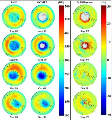
Figure 9 shows the averaged monthly distributions of total ozone in DU for both IASI 10

and GOME-2 (first and second columns respectively) over the Antarctic region for the ozone hole season, August through to November 2009. Despite the effect of GOME-2 being unable to measure completely during the polar night, which is visible from the data gaps at the centre of the Antarctic for August and September, both instruments show similar structures for the ozone total columns. As expected for each month max-15

imum total ozone is observed in the polar vortex and minimum total ozone is observed within the ozone hole. The temporal and spatial evolution of the ozone hole throughout the period is also well observed by both instruments. It is worth noting for August and September the data gaps visible in the GOME-2 data set can be filled using assimi-lated data and for October and November su_fficient light is available so that almost full 20

retrievals from GOME-2 are possible.

The third column in Fig. 9 presents the percentage difference between IASI and GOME-2. Despite both instruments observing similar structures for all months, IASI in general measures between 5 %–10 % higher ozone concentrations and observes a much stronger vortex surrounding the ozone hole than GOME-2. The predominant 25

(14)

AMTD

4, 4717–4752, 2011

IASI

C. Scannell et al.

◭ ◮

Discussion

P

a

per

|

Dis

cussion

P

a

per

|

Discussion

P

a

per

|

Discussio

n

P

a

per

|

IASI measures a slightly larger elongated ozone hole than GOME-2. In the vortex for all months a positive bias of approximately 7/8 % is also observed as IASI measures larger concentrations than GOME-2. However in general the difference between the two instruments remains below 10 %. Previous studies have shown such a bias (of approximately 5 %) exists between TIR and UV-vis observations andmay be due to 5

discrepancies of spectroscopic parameters such as differences in the absorbtion cross section and line parameters (e.g. Schneider et al., 2008; Anton, 2011). A recent study by Massart et al. (2009), also found that IASI tends to overestimate the ozone total columns in comparison to a model forced by the total columns retrieved from MLS (mi-crowave limb sounder) and SCIAMACHY (Scanning Imaging Absorption spectrometer 10

for Atmospheric Cartography).

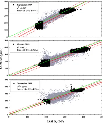
Figure 10 presents a statistical comparison between IASI and GOME-2 ozone to-tal columns that was performed for September, October and November of 2009. The correlation coe_fficients and the bias about the mean are inset into the graph for each month. The black data below 220 DU and above 320 DU represent ozone values within 15

the ozone hole and in its associated vortex respectively. The grey data represents all other data south of 45◦_{S, the area for which the ozone hole is defined, which do not lie}

within the hole or vortex regions. The linear regression for each month (solid red lines), the confidence intervals (dashed red lines) and the 1:1 ratio reference line (dashed green line) are also presented in the figure. It is clear from the strong correlation coef-20

ficients for each month (r2₌0.967, r2₌0.973 and r2₌0.975) that IASI and GOME-2 are closely comparable throughout the entire ozone hole region and period. Based on these regression lines IASI shows a slight positive bias as previously highlighted by the relative di_fference plots.

At the ozone hole region both instruments compare quite well, though slight diff er-25

(15)

AMTD

4, 4717–4752, 2011

IASI

C. Scannell et al.

◭ ◮

Discussion

P

a

per

|

Dis

cussion

P

a

per

|

Discussion

P

a

per

|

Discussio

n

P

a

per

|

between the two instruments and efforts should be made to fully understand this, some di_fferences between the instruments can be attributed to the di_fferent modes of obser-vation which have not been accounted for in this analysis. For example both instru-ments have a different ground footprint and observation geometry and thus are subject to di_fferent cloud contamination and probe di_fferent air masses. Both instruments also 5

have di_fferent vertical sensitivities, IASI has a maximum sensitivity to the ozone profile in the upper troposphere–lower stratosphere while GOME-2 has a maximum sensitivity in the stratosphere.

5 Comparison with ozone sondes

The in-situ ozone-sonde profile measurements used in this study are from the WOUDC 10

(World Ozone and Ultra Violet Radiation Data Centre) data base and the location of each indicated in figure 11 are the German Neumayer station (78◦39′S; 08◦15′W, WMO no. 323), the Australian Davis station (68◦35′S; 77◦58′E, WMO no. 450) and the Argentinian USH station (54◦₈₈′_{S; 68}◦₁₉′_{W, WMO no. 339) in blue, red and green}

respectively. Each station is equipped with electrochemical concentration cell (ECC) 15

ozone-sondes which utilize the oxidation reaction of ozone with potassium iodide to de-termine the ozone concentration throughout the profile. These ozone-sondes measure the profile of ozone up to 30 km into the atmosphere.

It should be noted that over this particular region finding a collocation between IASI, GOME-2 and an ozone sonde was not possible because ozone sonde measurements 20

are not daily and GOME-2 due to its geometry may be scanning a di_fferent location to IASI and the ozone sonde. The primary challenge with comparing IASI and ozone sonde measurements is the relatively small number of co-incident measurements be-tween satellite and sondes in the Antarctic. A set of strict co-incidence criteria were applied so as to correctly compare the IASI retrieved ozone profiles with the in-situ 25

(16)

AMTD

4, 4717–4752, 2011

IASI

C. Scannell et al.

◭ ◮

Discussion

P

a

per

|

Dis

cussion

P

a

per

|

Discussion

P

a

per

|

Discussio

n

P

a

per

|

and co-located in time to within 6 h were chosen. For the cases where 2 or more such IASI profiles fit the co-locations an averaged profile was calculated for the comparison. Secondly to make comparisons between IASI and the ozone-sondes, the di_fference in vertical resolution and sensitivity between the two data sets must be accounted for. For this reason the IASI averaging kernel and constraints are applied to the ozone-5

sonde data following Eq. (2), producing a vertical profile that represents what IASI would measure for the same air sampled by the sonde. For a more in-depth description of this method see Rodgers (2000).

Finally it should be noted that the sonde data are supplied in units of ozone partial pressure on a vertical scale of atmospheric pressure while the IASI data are supplied in 10

molecules cm−3_{on a vertical scale of atmospheric height. Therefore before the}

ozone-sonde data can be convolved with the IASI averaging kernels , the vertical scales and the units must be homogenized via a simple extrapolation and unit conversion as follows:

n ₌ 10−9 Ppart

kT (3)

15

wherenis in molecules cm−1_,_P

part is ozone in partial pressure in hPa,k is the Boltz-mann constant (1.3807×10−23J K−1molecule−1) andT is the temperature in K.

Figure 12 shows an example of a IASI and ozone-sonde profiles (red and blue pro-files respectively) taken from within the ozone hole during September 2009. The IASI a priori profile (dotted black profile) is also represented for each location. As previously 20

discussed in Sect. 2.2 retrieving ozone profiles with IASI over the ice can prove di_fficult thus it should be noted that the averaging kernels for each collocation between IASI and the ozone-sonde were closely studied and only those measurements with well defined averaging kernels and DOFs greater than or equal to 3 were chosen for this comparison.

25

(17)

AMTD

4, 4717–4752, 2011

IASI

C. Scannell et al.

◭ ◮

Discussion

P

a

per

|

Dis

cussion

P

a

per

|

Discussion

P

a

per

|

Discussio

n

P

a

per

|

instruments such as the notable decrease in ozone concentrations between 15–20 km, however IASI does over estimate slightly in the lower troposphere for all cases.

In the vortex (Fig. 13) for the USH and Davis stations IASI compares well to the convolved ozone sondes with only marginal differences in shape and magnitude. In the troposphere there is almost no difference while in the stratosphere IASI slightly over 5

estimates in comparison to the USH station and under estimates for the Davis station. A percentage difference calculation between the IASI and the convolved sonde ozone profiles for each station found that IASI and the sondes compare to within 20 % and within 30 % for the other two cases and demonstrates just how accurately IASI can estimate the shape and size of ozone profiles during the ozone hole period.

10

6 Summary and conclusion

This paper presents an assessment of the capabilities of IASI to perform continuous, precise measurements of the ozone hole. IASI will fly continuously for the next 10 years (on MetOp-B and -C), which should be followed by an improved IASI instrument in the 2019 timeframe. As already reported for CO in Pommier et al. (2010), polar regions are 15

at the same time easy to observe as they are well covered by the MetOp polar orbiting satellite, but on the other hand difficult to process due to the specific low temperature and thermal contrast conditions and frozen surfaces that impact the radiance spectra. In this work, the FORLI-O3 retrieval scheme was utilized. This retrieval algorithm allows the processing of global distributions of ozone two times per day, in near real time, from 20

all the IASI spectra with cloud contamination of less than 13 %.

In this work we analyze the IASI ozone total columns distributions over the Antarctic to study the ozone hole evolution in 2008, 2009 and 2010. Our results highlight the capability of IASI to capture very precisely the short term spatial and temporal variabil-ity of the ozone hole development, including during the polar night. Data comparisons 25

(18)

AMTD

4, 4717–4752, 2011

IASI

C. Scannell et al.

◭ ◮

Discussion

P

a

per

|

Dis

cussion

P

a

per

|

Discussion

P

a

per

|

Discussio

n

P

a

per

|

and size of the hole. A detailed comparison for 2009 provided correlation coefficients of 0.97 for September, October and November. For this region IASI showed an aver-age positive bias of approximately 7 %. This is in keeping with previous research by Boynard et al. (2009) who found an average positive bias of between 3 %–5 % on a global scale.

5

The retrieval of ozone vertical profiles from IASI spectra collocated with ozone sonde measurements for September 2009 was also performed. Here we found that IASI showed good agreement with the sonde measurements from the troposphere to the stratosphere, with the di_fference between IASI and the sondes being less than 30 % within the hole itself. IASI was also found to be very sensitive to the ozone profile in 10

the lower stratosphere between 15–20 km, remarkably capturing the vertical extent of the ozone hole, as shown by the good agreement with the ozone sondes.

Such continuous IASI ozone measurements are complementing existing data in the long term trend assessment of ozone which suggests that the ozone hole expansion and ozone loss rates have appeared to have stopped (WMO, 2010).

15

Work is in progress to combine the IASI and GOME-2 profile products to derive improved profiles. Theoretical studies have shown that improvements in measuring the troposphere could be achieved via the combination of complimentary UV and TIR measurements (Zhang et al., 2010; Worden et al., 2007). This study is a first step in identifying the potential difficulties encountered when dealing with real observations. 20

Acknowledgements. IASI has been developed and built under the responsibility of the

Cen-tre National des Etudes Spatiales (CNES, France). It is flown onboard the MetOp satellites as part of the EUMETSAT Polar System. The IASI level 1 data are distributed in near real time by EUMETSAT through the Eumetcast dissemination system. The authors acknowl-edge the Ether French atmospheric database (http://ether.ipsl.jussieu.fr) for providing the IASI 25

(19)

AMTD

4, 4717–4752, 2011

IASI

C. Scannell et al.

◭ ◮

Discussion

P

a

per

|

Dis

cussion

P

a

per

|

Discussion

P

a

per

|

Discussio

n

P

a

per

|

and are publically available (http://www.woudc.org, http://croc.gsfc.nasa.gov/shadoz and http: //www.esrl.noaa.gov/gmd). All the agencies cited above are acknowledged for providing data. The research in France was conducted with the financial support of CNES. The research in Belgium was funded by the “Actions de Recherche Concert ées” (Communaut é Française), the Fonds National de la Recherche Scientifique (FRS-FNRS F.4511.08), the Belgian State Federal 5

Office for Scientifique, Technical and Cultural Affairs and the European Space Agency (EAS-Prodex C90-327).

The publication of this article is financed by CNRS-INSU. 10

References

Ant ón, M., Loyola, D., Clerbaux, C., L ópez, M., Vilaplana, J. M., Ba ñ ón, M., Hadji-Lazaro, J., Valks, P., Hao, N., Zimmer, W., Coheur, P. F., Hurtmans, D., and Alados-Arboledas, L.: Validation of the Metop-A total ozone data from GOME-2 and IASI using reference ground-based measurements at the Iberian Peninsula, Remote Sens. Environ., 115, 1380–1386, 15

2011.

Balis, D. S. and Bojkov , R. D. : Characteristics of Antarctic Spring ozone decline from satellite and ground based measurements from the appearance of the “ozone hole” up to December 2001, edited by: Harris, N., Amanatidis, G., and Levine, J., Europ. Com. Air Pollution Re-search Report No. 79, Proc. of the 6th Europ. Symp. on Stratospheric Ozone in Goeteborg, 20

Sweeden, 39–42, 2003.

Boynard, A., Clerbaux, C., Coheur, P.-F., Hurtmans, D., Turquety, S., George, M., Hadji-Lazaro, J., Keim, C., and Meyer-Arnek, J.: Measurements of total and tropospheric ozone from IASI: comparison with correlative satellite, ground-based and ozonesonde observations, Atmos. Chem. Phys., 9, 6255–6271, doi:10.5194/acp-9-6255-2009, 2009.

(20)

AMTD

4, 4717–4752, 2011

IASI

C. Scannell et al.

◭ ◮

Discussion

P

a

per

|

Dis

cussion

P

a

per

|

Discussion

P

a

per

|

Discussio

n

P

a

per

|

British Antarctic Survey: Ozone bulletin, http://www.theozonehole.com/2010ozone.htm, last ac-cess: July 2011, The Ozone Hole, 2010.

Clarisse, L., Coheur, P. F., Prata, A. J., Hurtmans, D., Razavi, A., Phulpin, T., Hadji-Lazaro, J., and Clerbaux, C.: Tracking and quantifying volcanic SO2with IASI, the September 2007

eruption at Jebel at Tair, Atmos. Chem. Phys., 8, 7723–7734, doi:10.5194/acp-8-7723-2008, 5

2008.

Clarisse, L., Clerbaux, C., Dentener, F., Hurtmans, D., and Coheur, P.-F.: Global amo-nia distribution derived from infrared satellite observations, Nat. Geosci., 2, 479–483, doi:10.1038/NGEO551, 2009.

Clerbaux, C., Boynard, A., Clarisse, L., George, M., Hadji-Lazaro, J., Herbin, H., Hurtmans, D., 10

Pommier, M., Razavi, A., Turquety, S., Wespes, C., and Coheur, P.-F.: Monitoring of atmo-spheric composition using the thermal infrared IASI/MetOp sounder, Atmos. Chem. Phys., 9, 6041–6054, doi:10.5194/acp-9-6041-2009, 2009.

Coheur, P.-F., Barret, B., Turquety, S., Hurtmans, D., Hadji-Lazaro, J., and Clerbaux, C.: Re-trieval and characterization of ozone vertical profiles from a thermal infrared nadir sounder, 15

J. Geophys. Res., 110, D24303, doi:10.1029/2005JD005845, 2005.

Coheur, P.-F., Clarisse, L., Turquety, S., Hurtmans, D., and Clerbaux, C.: IASI measurements of reactive trace species in biomass burning plumes, Atmos. Chem. Phys., 9, 5655–5667, doi:10.5194/acp-9-5655-2009, 2009.

De Laat, A. T. J., van der A, R. J., Allaart, M. A. F., van Weele, M., Benitez, G. C., Casic-20

cia, C., Paes Leme, N. M., Quel, E., Salvador, J., and Wolfram, E. : Extreme sunbathing: Three weeks of small total O3 columns and high UV radiation over the southern tip of

South America during the 2009 Antarctic O₃hole season, Geophys. Res. Lett., 37, L14805, doi:10.1029/2010GL043699, 2010.

Feng, W., Chipperfield, M. P., Davies, S., Sen, B., Toon, G., Blavier, J. F., Webster, C. R., Volk, 25

C. M., Ulanovsky, A., Ravegnani, F., von der Gathen, P., Jost, H., Richard, E. C., and Claude, H.: Three-dimensional model study of the Arctic ozone loss in 2002/2003 and comparison with 1999/2000 and 2003/2004, Atmos. Chem. Phys., 5, 139–152, doi:10.5194/acp-5-139-2005, 2005.

Fortuin, J. P. F. and Kelder, H.: An ozone climatology based on ozone sonde and satellite 30

(21)

AMTD

4, 4717–4752, 2011

IASI

C. Scannell et al.

◭ ◮

Discussion

P

a

per

|

Dis

cussion

P

a

per

|

Discussion

P

a

per

|

Discussio

n

P

a

per

|

George, M., Clerbaux, C., Hurtmans, D., Turquety, S., Coheur, P.-F., Pommier, M., Hadji-Lazaro, J., Edwards, D. P., Worden, H., Luo, M., Rinsland, C., and McMillan, W.: Carbon monoxide distributions from the IASI/METOP mission: evaluation with other space-borne remote sen-sors, Atmos. Chem. Phys., 9, 8317–8330, doi:10.5194/acp-9-8317-2009, 2009.

Liu, X., Bhartia, P. K., Chance, K., Froidevaux, L., Spurr, R. J. D., and Kurosu, T. P.: Valida-5

tion of Ozone Monitoring Instrument (OMI) ozone profiles and stratospheric ozone columns with Microwave Limb Sounder (MLS) measurements, Atmos. Chem. Phys., 10, 2539–2549, doi:10.5194/acp-10-2539-2010, 2010.

Massart, S., Clerbaux, C., Cariolle, D., Piacentini, A., Turquety, S., and Hadji-Lazaro, J.: First steps towards the assimilation of IASI ozone data into the MOCAGE-PALM system, Atmos. 10

Chem. Phys., 9, 5073–5091, doi:10.5194/acp-9-5073-2009, 2009.

Maturilli, M., Neuber, R., Massoli, P., Cairo, F., Adriani, A., Moriconi, M. L., and Di Don-francesco, G.: Differences in Arctic and Antarctic PSC occurrence as observed by lidar in Ny- ˚Alesund (79◦_{N, 12}◦_{E) and McMurdo (78}◦_{S, 167}◦_{E), Atmos. Chem. Phys., 5, 2081–2090,} doi:10.5194/acp-5-2081-2005, 2005.

15

McPeters, R. D. and Labow, G. J.: An assessment of the accuracy of 14.5 years of nimbus 7 TOMS version 7 ozone data by comparison with the Dobson network, Geophys. Res. Lett., 23, 3695–3698, 1996.

McPeters, R. D., Labow, G. J., and Logan, J. A.: Ozone climatological profiles for satellite retrieval algorithms, J. Geophys. Res., 112, D05308, doi:10.1029/2005JD006823, 2007. 20

Newman, P. A., Nash, E. R., Kawa, S. R., Montzka, S. A., and Schauffler, S. M.: When will the ozone hole recover?, Geophys. Res. Lett., 33, L12814, doi:10.1029/2005GL025232, 2006. Newman, P. A., Rex, M., Canziani, P. O., Carslaw, K. S., Drdla, K., Godin-Beekmann, S.,

Golden, D. M., Jackman, C. H., Kreher, K., Langematz, U., M ¨uller, R., Nakane, H., Orsolini, Y. J., Salawitch, R. J., Santee, M. L., von Hobe, M., and Holden, S.: Polar Ozone: Past and 25

Present, Chapter 4 in Scientific Assessment of Ozone Depletion: 2006, Global Ozone Re-search and Monitoring Project – Report No. 50, World Meteorological Organization, Geneva, Switzerland, 2007.

Newman, P. A., Oman, L. D., Douglass, A. R., Fleming, E. L., Frith, S. M., Hurwitz, M. M., Kawa, S. R., Jackman, C. H., Krotkov, N. A., Nash, E. R., Nielsen, J. E., Pawson, S., Stolarski, R. S., 30

(22)

AMTD

4, 4717–4752, 2011

IASI

C. Scannell et al.

◭ ◮

Discussion

P

a

per

|

Dis

cussion

P

a

per

|

Discussion

P

a

per

|

Discussio

n

P

a

per

|

Pommier, M., Law, K. S., Clerbaux, C., Turquety, S., Hurtmans, D., Hadji-Lazaro, J., Co-heur, P.-F., Schlager, H., Ancellet, G., Paris, J.-D., N ´ed ´elec, P., Diskin, G. S., Podolske, J. R., Holloway, J. S., and Bernath, P.: IASI carbon monoxide validation over the Arctic dur-ing POLARCAT sprdur-ing and summer campaigns, Atmos. Chem. Phys., 10, 10655–10678, doi:10.5194/acp-10-10655-2010, 2010.

5

Razavi, A., Clerbaux, C., Wespes, C., Clarisse, L., Hurtmans, D., Payan, S., Camy-Peyret, C., and Coheur, P. F.: Characterization of methane retrievals from the IASI space-borne sounder, Atmos. Chem. Phys., 9, 7889–7899, doi:10.5194/acp-9-7889-2009, 2009.

Razavi, A., Karagulian, F., Clarisse, L., Hurtmans, D., Coheur, P. F., Clerbaux, C., M ¨uller, J. F., and Stavrakou, T.: Global distributions of methanol and formic acid retrieved for the 10

first time from the IASI/MetOp thermal infrared sounder, Atmos. Chem. Phys., 11, 857–872, doi:10.5194/acp-11-857-2011, 2011.

Rothman, L. S., Jacquemart, D., Barbe, A., Benner, D. C., Birk, M., Brown, L. R., Carleer, M. R., Chackerian Jr., C., Chance, K., Coudert, L. H., Dana, V., Devi, V. M., Flaud, J.-M., Gamache, R. R., Goldman, A., Hartman, J.-M., Jucks, K. W., Maki, A. G., Mandin, J.-Y., Massie, S. 15

T., Orphal, J., Perrin, A., Rinsland, C. P., Smith, M. A. H., Tennyson, J., Tolchenov, R. N., Toth, R. A., Vander Auwera, J., Varanasi, P., and Wagner, G.: The HITRAN 2004 molecular spectroscopic database, J. Quant. Spectrosc. Ra., 96, 139–204, 2005.

Rothman, L. S., Gordon, I. E., Barbe, A., Benner, D. C., Bernath, P. F., Birk, M., Boudon, V., Brown, L. R., Campargue, A., Champion, J.-P., Chance, K., Coudert, L. H., Dana, V., Devi, 20

V. M., Fally, S., Flaud, J.-M., Gamache, R. R., Goldman, A., Jacquemart, D., Kleiner, I., Lacome, N., Lafferty, W. J., Mandin, J.-Y., Massie, S. T., Mikhailenko, S. N., Miller, C. E., Moazzen-Ahmadi, N., Naumenko, O., Nikitin, A. V., Orphal, J., Perevalov, V. I., Perrin, A., Predoi-Cross, A., Rinsland, C. P., Rotger, M., Simeckov ´a, M., Smith, M. A. H., Sung, K., Tashkun, S. A., Tennyson, J., Toth, R. A., Vandaele, A. C., and Vander Auwera, J.: The 25

HITRAN 2008 molecular spectroscopic database, J. Quant. Spectrosc. Ra., 110, 533–572, 2009.

Schneider, M., Redondas, A., Hase, F., Guirado, C., Blumenstock, T., and Cuevas, E.: Com-parison of ground-based Brewer and FTIR total column O3 monitoring techniques, Atmos.

Chem. Phys., 8, 5535–5550, doi:10.5194/acp-8-5535-2008, 2008. 30

(23)

AMTD

4, 4717–4752, 2011

IASI

C. Scannell et al.

◭ ◮

Discussion

P

a

per

|

Dis

cussion

P

a

per

|

Discussion

P

a

per

|

Discussio

n

P

a

per

|

van Roozendael, M., Loyola, D., Spurr, R., Balis, D., Lambert, J. C., Livschitz, Y., Valks, P., Ruppert, T., Kenter, P., Fayt, C., and Zehner, C.: Ten years of GOME/ERS2 total ozone data: the new GOME data processor (GDP) version 4: I. Algorithm description, J. Geophys. Res., 111, D14311, doi:10/1029/2005JD006375, 2006.

Wan, Z.: New refinements and validation of the MODIS land surface temperature/emissivity 5

products, Remote Sens. Environ., 512, 59–74, 2008.

Wespes, C., Hurtmans, D., Clerbaux, C., Santee, M. L., Martin, R. V., and Coheur, P. F.: Global distributions of nitric acid from IASI/MetOP measurements, Atmos. Chem. Phys., 9, 7949-7962, doi:10.5194/acp-9-7949-2009, 2009.

Worden, J., Liu, X., Bowman, K., Chance, K., Beer, R., Eldering, A., Gunson, M., and Worden, 10

H.: Improved tropospheric ozone profile retrievals using OMI and TES radiances, Geophys. Res. Lett., 34, L01809, doi:10.1029/2006GL027806, 2007.

WMO – World Meteorological Organization: Scientific assessment of ozone depletion, Global Ozone Res. Monit. Proj., Rep. 47, Geneva, Switzeland, 2002.

WMO – World Meteorological Organization: Nohende Ajavon, A.-L., Newman, P. A., Pyle, J. A., 15

and Ravishankara, A. R. (Assessment cochairs): Scientific assessment of ozone depletion, Global ozone and research and monitoring project, Report No. 52, 2010.

Zhang, L., Jacob, D. J., Liu, X., Logan, J. A., Chance, K., Eldering, A., and Bojkov, B. R.: Intercomparison methods for satellite measurements of atmospheric composition: appli-cation to tropospheric ozone from TES and OMI, Atmos. Chem. Phys., 10, 4725–4739, 20

(24)

AMTD

4, 4717–4752, 2011

IASI

C. Scannell et al.

Title Page Abstract Introduction Conclusions References Tables Figures ◭ ◮ ◭ ◮ Back Close Full Screen / Esc

Printer-friendly Version Interactive Discussion Discussion P a per | Dis cussion P a per | Discussion P a per | Discussio n P a per | Observerd Fitted R a d ia n c e ( x 1 0

-4 W

/

c

m

2 s

r m -1 ) 2 2 .5 3 3 .5 4 4 .5 5 5 .5 6

Wavenumber (cm-1

)

1025 1030 1035 1040 1045 1050 1055 1060 1065 1070 1075

R e si d u a l -0 .0 8 0 0 .0 8

Fig. 1. Example of the intense ozone band region (1025 cm−1_{–1075 cm}−1_{) of a typical IASI}

(25)

AMTD

4, 4717–4752, 2011

IASI

C. Scannell et al.

◭ ◮

Discussion

P

a

per

|

Dis

cussion

P

a

per

|

Discussion

P

a

per

|

Discussio

n

P

a

per

|

Fig. 2. Antarctic projections of IASI total ozone column distribution retrieved from the Neural

Network scheme (left) and the FORLI-O3 scheme (right). Data are averaged over a 1◦

(26)

AMTD

4, 4717–4752, 2011

IASI

C. Scannell et al.

◭ ◮

Discussion

P

a

per

|

Dis

cussion

P

a

per

|

Discussion

P

a

per

|

Discussio

n

P

a

per

|

Fig. 3. Illustration of two spectra in radiances, taken over the Antarctic. The blue spectrum

(27)

AMTD

4, 4717–4752, 2011

IASI

C. Scannell et al.

◭ ◮

Discussion

P

a

per

|

Dis

cussion

P

a

per

|

Discussion

P

a

per

|

Discussio

n

P

a

per

|

Fig. 4. Left panel: Antarctic projection of the IASI DOFs distribution. Middle and right panel:

(28)

AMTD

4, 4717–4752, 2011

IASI

C. Scannell et al.

◭ ◮

Discussion

P

a

per

|

Dis

cussion

P

a

per

|

Discussion

P

a

per

|

Discussio

n

P

a

per

|

Fig. 5.Antarctic projection of IASI total ozone columns (DU) retrieved from the FORLI-O3

algo-rithm. Data are averaged over a 1◦

(29)

AMTD

4, 4717–4752, 2011

IASI

C. Scannell et al.

◭ ◮

Discussion

P

a

per

|

Dis

cussion

P

a

per

|

Discussion

P

a

per

|

Discussio

n

P

a

per

|

Fig. 6. Daily time series from the beginning of August 2008 to the end of December 2010

(30)

AMTD

4, 4717–4752, 2011

IASI

C. Scannell et al.

◭ ◮

Discussion

P

a

per

|

Dis

cussion

P

a

per

|

Discussion

P

a

per

|

Discussio

n

P

a

per

|

Fig. 7.Antarctic projections of the total ozone column distributions averaged over 3 day periods

in October 2009. The change from a circular to elliptical rotation and back again is clearly visible from the distributions. Data are averaged over a 1◦

(31)

AMTD

4, 4717–4752, 2011

IASI

C. Scannell et al.

◭ ◮

Discussion

P

a

per

|

Dis

cussion

P

a

per

|

Discussion

P

a

per

|

Discussio

n

P

a

per

|

Fig. 8. Temporal evolution of the area of the ozone hole (defined as lower than 220 DU) as

measured from IASI (solid line) and GOME-2 (dashed line) for 2008 (green), 2009 (blue) and 2010 (red). This data set is compiled from weekly averaged data from a 1◦

(32)

AMTD

4, 4717–4752, 2011

IASI

C. Scannell et al.

◭ ◮

Discussion

P

a

per

|

Dis

cussion

P

a

per

|

Discussion

P

a

per

|

Discussio

n

P

a

per

|

Fig. 9. Antarctic projections of IASI and GOME2 total ozone column monthly averaged

(33)

AMTD

4, 4717–4752, 2011

IASI

C. Scannell et al.

◭ ◮

Discussion

P

a

per

|

Dis

cussion

P

a

per

|

Discussion

P

a

per

|

Discussio

n

P

a

per

|

Fig. 10. Correlation between GOME-2 and IASI for September (top panel), October

(34)

AMTD

4, 4717–4752, 2011

IASI

C. Scannell et al.

◭ ◮

Discussion

P

a

per

|

Dis

cussion

P

a

per

|

Discussion

P

a

per

|

Discussio

n

P

a

per

|

Fig. 11.Geographic locations of the three ground based stations used for the IASI/ozone sonde

(35)

AMTD

4, 4717–4752, 2011

IASI

C. Scannell et al.

◭ ◮

Discussion

P

a

per

|

Dis

cussion

P

a

per

|

Discussion

P

a

per

|

Discussio

n

P

a

per

|

Fig. 12. Comparisons between IASI and ozone sonde profiles measured within the ozone

(36)

AMTD

4, 4717–4752, 2011

IASI

C. Scannell et al.

◭ ◮

Discussion

P

a

per

|

Dis

cussion

P

a

per

|

Discussion

P

a

per

|

Discussio

n

P

a

per

|

Fig. 13. Comparison between IASI and ozone sonde profiles measured within the ozone