FUNDAÇÃO GETULIO VARGAS
ESCOLA de PÓS-GRADUAÇÃO em ECONOMIA
Rafael de Vasconcelos Xavier Ferreira
Essays in Corporate Bankruptcy
Essays in Corporate Bankruptcy
Tese para obtenção do grau de doutor apresentada à Escola de Pós-Graduação em Economia
Área de concentração: Teoria Econômica Orientador: Aloisio P. Araujo
Ficha catalográfica elaborada pela Biblioteca Mario Henrique Simonsen/FGV
Ferreira, Rafael de Vasconcelos Xavier
Essays in Corporate Bankruptcy / Rafael de Vasconcelos Xavier Ferreira – 2014. 69f. Tese (Doutorado) – Fundação Getulio Vargas, Escola de Pós-Graduação em Economia. Orientador: Aloisio P. Araujo.
Inclui bibliografia.
1. Falência. 2. Créditos. 3. Direito e economia. I. Araujo, Aloisio Pessoa de, 1946- . II. Fundação Getulio Vargas, Escola de Pós-Graduação em Economia. III. Título.
Nas linhas seguintes – as últimas que escrevo para esta tese – gostaria de agradecer àqueles com quem este doutorado me deixou uma dívida de gratidão.
Primeiramente, quero agradecer aos meus pais. Desde que lhes contei, em 2005, da minha vontade de fazer mestrado e doutorado em economia, eles sempre me incentivaram, mesmo sabendo que a distância geográfica era condição necessária. Sem o apoio, em diversas dimen-sões, que recebi deles, chegar até aqui seria muito mais difícil, provavelmente impossível.
Obrigado também a Fred, pelo irmão querido que é.
Aos amigos Eduardo Cesar Maia, Leonardo Rabelo, Marcelo Correia, Marcelo Sandes e Renato Lima: obrigado pelas conversas, ainda durante o curso de graduação, que me fizeram ter certeza de que queria estudar economia a fundo.
Obrigado à Fundação Getulio Vargas (FGV) – e em especial à sua Escola de Pós-Graduação em Economia (EPGE) – pelo apoio institucional; e à Capes, ao CNPq e à FAPERJ pelo apoio financeiro imprescindível.
Quero também agradecer aos professores da EPGE, por terem me ensinado um método para aprender mais sobre o mundo que nos cerca. Em especial, destaco os professores Victor Filipe Martins-da-Rocha, Ricardo Cavalcanti, Luis H. B. Braido, Carlos Eugênio da Costa, Humberto Moreira e Marcelo Moreira.
Muito obrigado também ao meu professor orientador, Aloisio Araujo, pelo apoio e en-sinamentos que recebi como seu orientando, e pela dedicação com que desempenhou o seu papel.
Obrigado aos professores Flavio Cunha (University of Pennsylvania) e Bruno Funchal (FU-CAPE Business School), pelo muito que aprendi trabalhando com eles, em coautoria.
Obrigado a Marcia Waleria e a Andrea Machado, pela gentileza e pela presteza que de-monstraram sempre que precisei recorrer a elas.
Em especial, gostaria de agradecer também aos meus colegas de mestrado e doutorado. Ao longo desses anos, convivi na EPGE com algumas das pessoas mais inteligentes e mais generosas que conheço. Amigos sempre dispostos a responder uma dúvida, por mais banal que lhes pareça; a ajudar na demonstração de um teorema ou na aplicação de um método estatístico; ou a tornar mais clara a interpretação econômica quando ela teimava em se escon-der entre equações matemáticas. Obrigado pela amizade e pelos excelentes lembranças, que levarei sempre comigo.
Resumo
Esta tese é composta por três ensaios sobre o mercado de crédito e as instituições que regem bancarrota corporativa.
No capítulo um, trazemos evidências que questionam a ideia de que maiores níveis de proteção ao credor sempre promovem desenvolvimento do mercado de crédito. Desde a publicação dos artigos seminais deLa Porta et al.(1997,1998), a métrica de proteção ao credor que os autores propuseram – o índice de proteção ao credor – tem sido amplamente utilizada na literatura de Law and Finance como variável explicativa em modelos de regressão linear
em forma reduzida para determinar a correlação entre proteção ao credor e desenvolvimento do mercado de crédito. Neste artigo, exploramos alguns problemas com essa abordagem. Do ponto de vista teórico, essa abordagem geralmente supõe uma relação monotônica entre proteção ao credor e expansão do crédito. Nós apresentamos um modelo teórico para um mercado de crédito com seleção adversa em que um nível intermediário de proteção ao credor é capaz de implementar equilíbrios first best. Este resultado está de acordo com diversos
outros artigos teóricos, tanto em equilíbrio geral quanto em equilíbrio parcial. Do ponto de vista empírico, tiramos proveito das reformas realizadas por alguns países durante as décadas de 1990 e 2000 para implementar uma estratégia inspirada na literatura detreatment effectse
estimar o efeito sobre o valor de mercado e sobre a dívida de: i) permitir automatic stay a
firmas em recuperação; e ii) conceder aos credores o direito de afastar os administradores. Os resultados que obtivemos apontam para um impacto positivo deautomatic staysobre todas as
variáveis que dependem do valor de mercado da firma. Não encontramos efeito sobre dívida, e não encontramos efeitos significativos do direito de afastar administradores sobre valor de mercado ou dívida.
O capítulo dois avalia as consequências empíricas de uma reforma na lei de falências sobre um mercado de crédito pouco desenvolvido. No início de 2005, o Congresso Nacional brasi-leiro aprovou uma nova lei de falências, a lei 11.101/05. Usando dados de firmas brasileiras e não-brasileiras, nós estimamos, usando dois modelos diferentes, o efeito da reforma fali-mentar sobre variáveis contratuais e não-contratuais de dívida. Ambos os modelos produzem resultados similares. Encontramos um aumento no volume total de dívida e na dívida de longo prazo, e uma redução no custo de dívida. Não encontramos efeitos significativos sobre a estrutura de propriedade da dívida.
No capítulo três, desenvolvemos um modelo estimável de equilíbrio em search direcionado aplicado ao mercado de crédito, modelo este que pode ser usado para realizar avaliaçõesex ante de mudanças institucionais que afetem o crédito (como reformas em leis de falência).
A literatura em economia há muito reconhece uma relação causal entre instituições (como leis e regulações) e desenvolvimento dos mercados financeiros. Essa conclusão qualitativa é amplamente reconhecida, mas há pouca evidência de sua importância quantitativa. Com o nosso modelo, é possível estimar como contratos de dívida mudam em resposta a mudanças nos parâmetros que descrevem as instituições da economia. Também é possível estimar o impacto sobre investimentos realizados pelas firmas, bem como caracterizar a distribuição do tamanho, idade e produtividade das firmas antes e depois da mudança institucional. Como ilustração, realizamos um exercício empírico em que usamos dados de firmas brasileiras para simular o impacto de variações na taxa de recuperação de créditos sobre os valores médios e totais de dívida e capital das firmas. Encontramos dívida crescente e capital quase sempre também crescente na taxa de recuperação.
This thesis contains three chapters, each bringing an essay on credit markets and on the institutions governing corporate bankruptcy.
In chapter one, we bring some evidence to dispute the notion that increasing creditor pro-tection always promotes credit market development. Ever since the seminal works ofLa Porta et al.(1997,1998), the metric of creditor protection they proposed – the creditor rights index – has been widely used in the Law and Finance literature as explanatory variable in reduced form regression models to assess how creditor protection correlates to credit market devel-opment. We explore some problems with this approach. From a theoretical standpoint, it usually assumes a monotonic relation between creditor protection and financial development. We present a theoretical model for a credit market with adverse selection in which an interme-diate level of creditor protection is capable of implementing first best equilibria. This is in line with several other theoretical papers, both in general equilibrium and in partial equilibrium setups. From an empirical standpoint, we take advantage of legal reforms in some countries during the 1990’s and 2000’s to implement a strategy based on the treatment effects literature in order to investigate the impact in firm equity and debt of: (i) granting financially distressed firms the right to an automatic stay on assets during court-supervised reorganization; and (ii) allowing creditors to remove managers of firms in reorganization. We find that restricting automatic stay reduces all equity-related variables, and has no significant impact on debt. We find no significant impact of managerial removal on either debt or equity.
Chapter two evaluates the empirical consequences of a bankruptcy reform on a poorly developed credit market. In early 2005, the Brazilian Congress approved a new bankruptcy law. The new legislation increased creditor protection and improved the efficiency of the bankruptcy system. Using data from Brazilian and non-Brazilian firms, we estimate, using two different treatment effects models, the effects of the bankruptcy reform on contractual and non-contractual debt variables. In general, both models yield similar results. Concerning contractual debt variables, we found a significant increase in both total debt and long-term debt, and a reduction in the cost of debt. We found no effect in the loans’ ownership structure. Finally, in chapter three we develop an estimable equilibrium search model of credit that can be used to conduct ex-ante evaluation of institutional changes, such as bankruptcy laws. Economic literature has established a causal relationship between institutions (such as laws and regulations) and financial market development. While this qualitative conclusion is widely accepted in the literature, there is little evidence of its quantitative importance. With our framework, it is possible to estimate how debt contracts change in response to modifica-tions in credit-related institumodifica-tions. It is also possible to estimate how investments made by firms will be affected, as well as characterize the distribution of firm size, age, and produc-tivity before and after the institutional change. In an empirical exercise, we use data from Brazilian firms to simulate the effects of changing creditors recovery rates on the total and the mean values of both capital and debt. We find that debt increases with lower recovery rates. In most cases, the same is true for the stock of capital.
Lista de Figuras
1.1 Representation of the lender-borrower relationship as a game in the extensive
form. . . 5
1.2 Expected payoffs in bankruptcy and loss due to inefficiency . . . 10
1.3 Debt and equity; equilibria of the renegotiation subgame . . . 11
1.4 OLS regression intercepts . . . 14
2.1 Average length of insolvency procedures . . . 37
2.2 Evolution of bankruptcy related variables before and after th . . . 39
2.3 Ratio between corporate private credit and GDP (Brazil) . . . 42
2.4 Ratio between corporate private credit and GDP (all four countries) . . . 42
3.1 Timing of Events . . . 55
1.1 Example parameters . . . 9
1.2 All possible legal environments . . . 16
1.3 Summary of results . . . 18
1.4 Creditor Rights Index (1). . . 21
1.5 Creditor Rights Index (2). . . 22
1.6 Automatic stay on assets . . . 23
1.7 Automatic stay on assets (2) . . . 24
1.8 Restrictions on entering in reorganization (1) . . . 25
1.9 Restrictions on entering in reorganization (2) . . . 26
1.10 Secured creditors come first in liquidation (1) . . . 27
1.11 Secured creditors come first in liquidation (2) . . . 28
1.12 Managers removed in reorganization (1). . . 29
1.13 Managers removed in reorganization (2). . . 30
1.14 ATT estimates for the Creditor Rights Index . . . 31
1.15 ATT estimates for Automatic Stay on Assets . . . 32
1.16 ATT estimates for Managers being Removed in Reorganization . . . 33
2.1 Aggregate Time Series and Panel Data Estimates . . . 43
2.2 Difference-in-Differences Panel Robust Estimates . . . 46
2.3 Tests for Contractual Debt Variables . . . 47
2.4 Diff-in-Diff with Different Trends Panel Robust Estimates . . . 49
3.1 Distribution of debt contracts between types . . . 59
3.2 Distribution of debt contracts between floating and fixed rate . . . 60
3.3 Distribution of indexes for floating rate debt contracts . . . 60
3.4 Distribution of debt contrats according to security . . . 60
3.5 Simulation results forγ=1 . . . 64
Sumário
1 Creditor Protection, Debt and Equity 1
1.1 Introduction . . . 1
1.2 A basic model . . . 3
1.2.1 Bankruptcy . . . 4
1.2.2 Optimal debt contracts. . . 6
1.3 Numerical example . . . 9
1.4 Empirical considerations . . . 12
1.5 Estimation . . . 17
1.5.1 Data . . . 17
1.5.2 Results . . . 17
1.6 Concluding Remarks . . . 20
2 The Brazilian Bankruptcy Law Experience 34 2.1 Introduction . . . 34
2.2 The New Brazilian Bankruptcy Law . . . 36
2.3 Data Set . . . 40
2.4 Results . . . 41
2.4.1 Evidence from Aggregate Data . . . 41
2.4.2 Difference-in-Difference . . . 44
2.4.3 Diff-in-Diff with Different Trends . . . 48
2.5 Conclusion . . . 50
3 An equilibrium search framework for the analysis of credit markets in developing countries 51 3.1 Introduction . . . 51
3.2 The model . . . 52
3.2.1 Firms . . . 53
3.2.2 Lenders . . . 55
3.2.3 Recursive and Block-Recursive Equilibria . . . 56
3.3 Empirical strategy. . . 58
3.3.1 Data and descriptive statistics . . . 58
3.3.2 Estimation . . . 60
3.4 Some preliminary results . . . 63
3.5 Conclusion . . . 65
Creditor Protection, Debt and Equity
1.1 Introduction
In the last decades, many works have studied how different institutional designs relate to cre-dit market development. Two important landmarks in this effort were the papers ofLa Porta et al.(1997, 1998), that proposed a metric of creditor protection – the creditor rights index – that became widely used. These papers were followed by an extense empirical literature that included this metric as explanatory variable in reduced form regression models to assess how important creditor protection is in enhancing the supply of credit. A recurrent stylized fact from this literature is the idea that creditor protection – as measured byLa Porta et al. (1997,
1998) – is positively correlated to financial deepening.
In this chapter, we explore some problems with this approach, and propose a different empirical exercise. We take advantage of legal reforms in countries that changed their ban-kruptcy codes, so as to better control for unobservables and improve identification. From an empirical standpoint, we argue that an approach borrowed from the treatment effects litera-ture is capable of delivering far more trustworthy results than the usual cross-country OLS regressions frequently seen in the Law and Finance literature. In addition, we argue that using the creditor rights index as explanatory variable confounds the effects of individual legal fea-tures. Hence, we propose looking at each component of the index separately. In sections (1.4) and (1.5), we further describe this approach.
Another aspect we consider in this chapter is the impact of creditor protection on firm equity. Several papers focus on the correlation between creditor protection and debt, but equity is also important. If the borrowing firm declares bankruptcy, higher levels of credi-tor protection not only increase the expected payoff of credicredi-tors, but also decrease the resi-dual value that stockholders are entitled to claim. It is often the case that shareholders leave bankruptcy empty-handed, specially in more developed countries with strict enforcement of highly pro-creditor bankruptcy laws. As creditors become empowered and recovery rates become larger, incentives to liquidate the firm increase. Since stockholders are usually posi-tioned last or close to last in line to receive the proceedings of the sale of the firm’s assets, as liquidation probability increases, shareholders’ expected payoff decreases. This is expected to negatively impact equity prices. If we are interested in evaluating welfare properties of different legal environments, we must consider their effect on both equity and debt.
Our central empirical result is that although creditors rights in general are positively corre-lated with the total amount of credit in the economy – which is in some sense compatible with previous results – different pro-creditor provisions have different impacts on both creditors and debtors. In particular, we find that Chapter 11-like reorganizations with automatic stay have a positive impact on debtors, without hurting creditors too much. Therefore, we could see it as being welfare enhancing, from a purely empirical perspective.
2
the creditor rights index to be a good metric of creditor protection, there is no reason to expect financial deepening to be an increasing function of the index value. In sections (1.2) and (1.3), we present a dynamic model of debt with adverse selection in which liquidating of all distres-sed firms is inefficient. We show that giving firms a second chance, while preserving creditors rights in liquidation, can be described by a signaling mechanism capable of driving inefficient firms out of the market, while preserving the value of firms with high probability of suc-cess. This mechanism – roughly matching the reorganization procedure in Chapter 11 of U.S. Bankruptcy Code – results in lower interest rates, higher creditor payoffs and higher equity values, for legal environments in which a separating Bayesian Nash equilibrium emerges.
Both our empirical and theoretical results are compatible with the incomplete market mo-dels in which an intermediary level of creditor protection maximizes welfare. These momo-dels see creditor protection – and debtor punishment – as enforcement mechanisms designed to avoid widespread strategic default.1 When such mechanisms are too weak – like in countries
where creditors have few legal options or little incentive to exert those options – debtors are expected to default strategically more often. Anticipating higher default probabilities, poten-tial lenders would avoid lending in the first place, shrinking the credit market through the supply side. In cases like this, we should see improvements in creditor protection leading to more developed credit markets.2 They also play an important role in mitigating moral hazard
and in reducing the associated agency costs.
However, when the enforcement mechanisms are too strong, borrowers become wary of punishment, weakening the credit market through the demand side. The immediate implica-tion is that an intermediate level creditor protecimplica-tion is optimal if the objective is maximizing welfare.
Looking specifically at corporate bankruptcy, a feature that is often cited as an important characteristic of pro-creditor legal environments is the strict observance of the “Absolute Pri-ority Rule” (APR), a principle stating that debtholders should be paid before equityholders, in descending order of seniority. Legal systems that are prone to liquidating firms in finan-cial distress and follow the Absolute Priority Rule are often considered to be the pro-creditor benchmark. In general, from an ex-ante sense, there is a consensus that creditor-friendly ins-titutions are important to provide incentives. The main argument is that if bankruptcy is considered sufficiently threatening, managers are less inclined to take excessive risk, expro-priate cash flow from the firm, strategically default, or falsely report the firm’s true returns, to name a few. Also, since pro-creditor laws usually increase the recovery rate of credit claims in case of default, creditors can lend at lower rates, increasing the attractiveness of safer pro-jects, and limiting risk-taking. When capital markets work well, this pro-creditor approach to bankruptcy is known to produce both ex ante3and ex post efficient outcomes.4
However, in some cases (specially when capital markets do not work well), ex ante and ex post efficiency do not go hand in hand. From an ex-post sense, when default has already happened, a good bankruptcy law should maximize and preserve firm value, and also lead to welfare-increasing asset reallocation. An important goal of bankruptcy is to drive inefficient firms out of the market. But when firms are economically viable, it may be optimal to give managers and shareholders a second chance. This is the case of firms whose managers possess specific knowledge about the business and are the only ones capable of restructuring a firm 1See, e.g.,Dubey et al.(2005),Geanakoplos and Zame(2013) andAraujo et al.(2012b). For a brief summary of this argument, see alsoAraujo et al.(Forthcoming).
2In line with this argument, Araujo et al.(2012a) investigate what happened after the 2005 bankruptcy law reform in Brazil, country that had very poor enforcement mechanisms prior to the reform and enhanced creditor protection. This paper is chapter 2 of this thesis.
3Townsend(1979),Aghion and Bolton(1992), andHart and Moore(1994,1998), for instance, show that loan prices are lower when creditors can more easily force repayment. If creditors can expect higher recovery rates in those states of nature in which their debtors default, their expected payoff will also be higher. In this case, they would be able to afford lower loan prices without incurring in a negative expected profit.
that is more valuable as a going concern. It may also the case of firms that are going through a temporary financial distress and are having difficulties in obtaining financing, due to some sort of credit market friction. The same is true if creditors’ coordination problems lead to inefficient liquidations; or if the firm is going through temporary financial distress and is having difficulties in obtaining financing, due to some sort of credit market friction. These cases provide arguments for legal systems that allow for deviations of the Absolute Priority Rule, and favor firm reorganization rather than liquidation.
Thus, a good bankruptcy law must strike a balance between pro-creditor and pro-debtor features, so as to provide the right incentives for both creditors and debtors, while avoiding inefficient liquidations. In the next section, we detail this point a bit further, with the aid of a dynamic model of debt and equity with adverse selection during bankruptcy procedures.
1.2 A basic model
To illustrate our main point, we present a model economy populated by two types of risk-neutral agents: borrowers and lenders. Time is discrete, and goes on for three periods t ∈ {0,1,2}.
Each borrower is endowed with a project – whose size is normalized to one – yielding a per-period random (gross) return ofYt ∈ {yL,yH}, fort > 0 andyL <1< yH. The
probabili-ties of these outcomes, however, are not the same for all projects. They differ according to each borrower’s type, which is privately observed (at the end of the initial periodt =0) and
repre-sented by θ ∈ Θ ≡ {θG,θB}. If a borrower is of type θi, withi∈ {G,B}, his project yieldsyH
with probabilitypi, andyLwith probability(1−pi)and Pr(θ =θG)≡ pG> pB ≡Pr(θ= θB).
The distribution of types in the economy is represented by the ex-ante probability that the borrower is of good type, denotedq∈(0,1).
Borrowers are assumed to be cash-constrained, so they must start by seeking lenders to finance their projects. Att = 0, they make the first move, by offering the lender a standard debt contract. In our setup, a debt contract is entirely described by the return R promised
to be paid by the borrower to the lender in the final period if the project is successful (i.e., if both realizations of the random return are equal toyH). We assume the lender has access to a
risk-free asset, with gross return equal to one.
The lender then decides whether to accept or reject the borrower’s offer. If he rejects, they both get zero and the game ends.
If the lender accepts the proposed debt contract, the borrower makes the investment in the project and finds out his typeθ, before moving to the next period.
Att =1, the first realization of the random return,Y1, is known to all. Somewhat similarly
to Bolton and Scharfstein (1990), if Y1 = yL the debtor undergoes a bankruptcy procedure,
whose final outcome can be either the continuation of the project or its liquidation, depending on the characteristics of the legal system in place.5 Hence, following a bad outcome int = 1,
the project goes forward only if the court decides that debt renegotiation must take place. If, however, the realization ofY1 is yH, then the firm continues to the next and final period. In
this final period, ifY2 = yH, then the project’s cash flow will be higher than the debtR, and
the creditor is paid. We assume there are no enforcement issues, meaning that the debtor cannot refrain from honoring the contract and paying the creditor’s claim. If, however, the final realization of the random return is a bad one, there is no possibility of any bankruptcy procedure other than liquidation, since the project has come to an end.
4
1.2.1 Bankruptcy
If the project’s first realization of the random return is a bad one (Y1 = yL), the debtor firm
will initiate a bankruptcy procedure. In our model, the bankruptcy procedure is characterized by a take-it-or-leave-it bargain game in which the first move is determined by the court. We parameterize the legal environment by a triple (ρ,λ,φ) ∈ [0,1]3 describing, respectively: the probabilityρthat the court will decide in favor of liquidating the firm; the percentageλof the project’s liquidation value creditors are entitled to claim; and the total liquidation valueφof the project, as a percentage of the total cash flow.
Therefore, when a debtor is taken to court, the court will rule, with probability ρ in fa-vor of liquidation, and with probability(1−ρ) in favor of a court-supervised renegotiation procedure.
If the court decides to allow for renegotiation, the debtor is entitled to make an offer
R1 ∈ [0,yHyL] to the project’s creditor to replace the original contract.6 The creditor, in his
turn, must decide whether to accept or reject this new offer. If the offer is accepted, the project can continue to the subsequent period; if the offer is rejected the project is liquidated.
In the last period, the final outcome is known. If the realizations of Y1 and Y2 are both
equal toyL, then the project is considered a failure, and it is liquidated; if onlyY1 resulted in
a bad outcome (and if the firm was not liquidated in the previous period), the creditor is paid what he is due,R1.
Therefore, the project will be liquidated in three cases:
1. During a bankruptcy procedure, when the court decides to liquidate the firm;
2. During a bankruptcy procedure, when the court decides to allow for renegotiation but the creditor rejects the debtor’s offer;
3. Following a bankruptcy procedure, when the final outcome of the project results in failure;
In all cases, liquidation comprises the sale of the project’s assets and the distribution of its proceedings according to some pre-established priority rule. In our model, the two para-meters describing the liquidation procedure areφ and λ. The former indicates the amount of resources raised by the sale, as a percentage of the project’s cash flow in the period of the liquidation; and the latter determines how much of these resources are transferred to the creditor.
More explicitly, if the project is liquidated in period 1, a total amount of φyL will be
available to be distributed among creditor and debtor. The creditor will receive λφyL, and
the debtor will receive(1−λ)φyL. A similar distribution pattern will be followed in the final
period, but with a lower cash flow, yieldingλφy2Lto the creditor and(1−λ)φy2Lto the debtor.
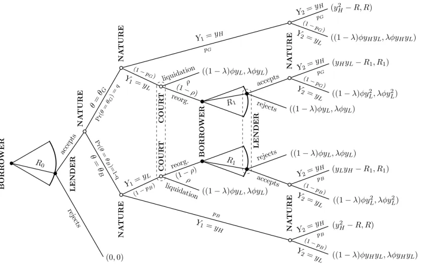
Figure1.1 displays the borrower-lender relationship as a incomplete information game in the extensive form.
We also make an important assumption regarding efficiency, to keep things interesting:
Assumption 1. AfterY1 = yL, the continuation value of the firm of typeθG ishigherthan its
liquidation value, and the continuation value of the firm of typeθBislowerthan its liquidation
value.
pGyLyH+ (1−pG)φy2L > φyL (1.1)
pByLyH+ (1−pB)φy2L < φyL (1.2)
5 B O R R O W E R
(0,0)
reje cts L E ND E R
((1−λ)φyHyL, λφyHyL) Y2 =
yL G)
Y1=yH
pG
((1−λ)φyL, λφyL)
liquidat ion
ρ
((1−λ)φy2L, λφy2L) Y2=
yL (1−
pG)
(yHyL−R1, R1)
Y2=yH pG
((1−λ)φyL, λφyL)
R1 (1− ρ) reorg. C O U R T C O U R T
Y1 = yL (1−p G) θ= θG NA TU R E NA TU R E NA TU R E Pr( θ= θG)
=
q
(y2H −R, R)
Y2=y H pB
((1−λ)φyHyL, λφyHyL) Y2 =
yL (1−
pB) Y1 =
yH
pB
((1−λ)φyL, λφyL)
liquidationρ
((1−λ)φy2L, λφy2L) accepts
rejects accepts
rejects
Y2= yL (1−
pB)
(yLyH −R1, R1)
NA TU R E NA TU R E
Y2=y H pB
((1−λ)φyL, λφyL)
B O R R O W E R L E ND E R R1 reorg. (1−ρ)
Y1= yL
(1−p
B) θ = θ B P r(θ = θB )= 1-q acce pts R0
6
It follows directly from this assumption that any legal system that implements the first-best allocation of resources must liquidate the firm of typeθB and allow the firm of typeθG to
continue.
1.2.2 Optimal debt contracts
In our environment, an optimal debt contract is the one that maximizes the debtor’s ex-ante payoff, subject to a participation constraint for the creditor. Let us denote by πdt and πct, respectively, the debtor’s and the creditor’s expected profits at the beginning of periodt. An optimal debt contract is one that satisfies:
R∗0 ∈arg max
R0
E
πd0(R0)] (1.3)
s.t. Eπc0(R0)≥1 (1.4)
We can rewrite the expected profit of the debtor as:
E
πd0(R0)] =qE
π0d(R0)|θ=θG
+ (1−q)E
πd0(R0)|θ=θB (1.5)
in which the conditional probabilities are determined as follows:
E
πd0(R0)|θ=θi
= piE
π1d(R0)|Y1=yH|θ=θi
+ (1−pi)E
πd1(R0)|Y1=yL,θ=θi
Similarly, we can define expected profit for the creditor in period 1, conditional on the realization of the first random return and on firm type. Let us denote byE
π1c|Y1 =yL,θ =θi
this conditional expected profit. It is not a function of the debt contract, because the creditor’s payoff in bankruptcy does not depend on the terms of the original contract R0. Since our objective function (1.3) is a non-increasing function of the creditor’s compensation R0, we
know the creditor’s participation constraint to be binding. Based on this, we know that any optimal debt contract must satisfy:
R∗0 = 1−λφy 2
L[(1−q)pB(1−pB) +qpG(1−pG)]
qp2G+ (1−q)p2B
− q(1−pG)E
πc1|yL,θG
+ (1−q)(1−pB)E
πc1|yL,θB
qp2G+ (1−q)p2B (1.6)
By substituting R∗0 in (1.5), we obtain the project’s value. These two expressions indicate
how debt and equity change, as functions of creditor’s and debtor’s payoffs in bankruptcy. Thus, we must determine how these payoffs vary with model parameters to determine how equity and debt relate to the legal environment.
If the court decides in favor of the debtor, he will be entitled to make an offer R1 to the
creditor. Given this offer, the creditor must choose whether to accept it or not. The creditor will accept the offer if doing so renders a higher payoff than that of rejecting the offer.
This scenario gives rise to a signaling mechanism somewhat similar to the one investigated bySpence (1973). In our case, the offer made by the informed party (the debtor firm) can be used to signal its type. In some cases, firms with a higher probability of success may find profitable to make an offer higher than the one we would see in a setting without adverse selection.
After receiving the signal R1, the creditor forms a belief that the firm making the offer is
based on this signal, the creditor decides to accept the firm’s offer if the expected payoff of accepting – computed based on the beliefsµ– is higher than the expected payoff of liquidating the firm. Thus, the offer will be accepted if:
µ(R1)[pGR1+ (1−pG)φλy2L] + [1−µ(R1)](pBR1+ (1−pB)φλy2L)≥λφyL (1.7)
The beliefµis formed by reevaluating the likelihood that the debtor is of the good type. We assume creditors update their beliefs in a Bayesian fashion, such that the updated probability of the creditor being of typeθGis given by:
qL≡Pr θ =θG|yL
= q(1−pG)
q(1−pG) + (1−q)(1−pB)
(1.8)
Pooling equilibria
If the debtor strategies are optimally chosen they must be consistent with some equilibrium. Here we have two possible types of equilibrium emerging. The first is a pooling equilibrium, in which the two types of firms will make the same offerR∗1(θG) = R1∗(θG). Upon receiving
the offer, the creditor forms its beliefs based on the updated probabilityqLand by interpreting
the debtor’s offer as an equilibrium strategy. Thus, it can easily be shown that in all polling equilibria,µ(R∗1) =qL.
From this condition, and from (1.7), we have the following necessary condition for a poo-ling equilibrium in which both types of firms make an offer that is accepted by the creditor:
R∗(θB) =R∗(θG)>
λφyL
1−yL qL(1−pG) + (1−qL)(1−pB)
qLpG+ (1−qL)pB
≡R¯P (1.9)
in which ¯RP determines a threshold for the creditor to accept the offer in a pooling
equili-brium. Thus, any offer below ¯RP is inconsistent with an acceptance pooling.
As for the debtors, if both types are willing to make the same offer – that they anticipate being accepted by the creditor – it must be advantageous for them to do so. That will happen when the payoff of both debtors accepting the offer exceeds the payoff of rejecting. Thus, we must have:
pG(yHyL−R1∗(θG)) + (1−pG)(1−λ)φy2L>(1−λ)φyL,
pB(yHyL−R∗1(θB)) + (1−pB)(1−λ)φy2L>(1−λ)φyL,
We can rewrite both inequalities to characterize theR∗1 that induces pooling:
R∗1 <yHyL−
(1−λ)φyL[1−(1−pG)yL]
pG
≡R1¯ (θG) (1.10)
R1∗< yHyL−
(1−λ)φyL[1−(1−pB)yL]
pB
≡R1¯ (θB) (1.11)
Since pG > pB, it can be easily shown that it suffices to have R∗1(θG) = R∗1(θB) < R1¯ (θB)
for a pooling equilibrium to arise. Therefore, from (1.9), we have that any offer R1consistent
with an acceptance pooling equilibrium must be in the interval [R˜P, ¯R1(θB)]. Furthermore,
any pooling equilibrium must have R∗1(θG) = R∗1(θB) = R˜P, since any offer higher than that
would be suboptimal.
8
Separating equilibria
The other type of equilibrium that can emerge is a separating equilibrium. Following any offerR1consistent with a separating perfect Bayesian equilibrium, the creditor’s beliefs about
the signaling agent’s type must be such that µ(R∗1(θG)) = 1 and µ(R∗1(θB)) = 0. So, any
equilibrium in which firms of different types make different offers will result in the Pareto efficient outcome of liquidating the firm of typeθB and preserving the firm of typeθG. If we
denote by π2d the debtors final payoff, any separating equilibria at the end of period t = 2, will have πd2(R∗1(θG),θG) = pG[yHyL−R1∗(θG)] + (1− pG)(1−λ)φy2L and π2d(R∗1(θB),θB) =
(1−λ)φyL.
For the firm of typeθGto prefer continuing into the subsequent period than being
liquida-ted, the repayment promiseR∗1(θG)made to the creditor would have to be lower than ¯R1(θG)
in (1.10). Also, the creditor will accept the firm’s offer in a separating equilibrium if we have:
R∗1(θG)>
φλyL[1−(1−pG)yL]
pG
≡R˜S(θG) (1.12)
In turn, the firm of type θB must find it optimal to offer its creditor a promiseR∗(θB)that
is below his acceptance threshold:
R∗(θB)≤
φλyL[1−(1−pB)yL]
pB
≡ R˜S(θB) (1.13)
Additionally, the payoff of choosing the same offer as the firm of typeθGmust not be
profi-table for the firm of typeθB. More specifically, we must haveπ2d(R∗1(θB),θB)>π2d(R∗1(θG),θB).
Since in every separating equilibriumπd2(R∗1(θB),θB) = (1−λ)φyL, this condition is satisfied
for everyR1∗(θG)> R1¯ (θB)in (1.11). Seeing thatpG> pB, it follows that ¯R1(θB)> R˜S(θG).
This last observation underlines the cost incurred by the firm of type θG when signaling
its type to the creditor. In an environment without asymmetric information, a lower offer equal to ˜RS(θG)would suffice for the firm to continue to the next period. In this environment,
however, such offer would give theθBfirm incentives to pool, by offering the same contract in
a similar situation.
Notice that the payoffπ2d(R∗1(θG),θG)is strictly decreasing in[R1¯ (θB), ¯R1(θG)]. Thus,R1∗(θG) =
¯
R1(θB) maximizes the payoff of the firm of type θG in this interval. And since the payoff
π2d(R1,θB) = (1−λ)φyLdoes not depend onR1, we can restrict our attention, without loss of
generality, to the equilibrium in whichR∗1(θB) =0.
Moral Hazard, reorganization costs and the efficiency of pro-creditor laws
Pro-liquidation legal environments are usually considered by the literature to be pro-creditor. The idea is that, in the presence of Moral Hazard, they are necessary to provide correct in-centives for debtors to behave and refrain from expropriating creditors. Our setup, however, does not include Moral Hazard. The only source of asymmetric information comes in the form of adverse selection. So, a pro-renegotiation legal environment could even end up being advantageous to the creditor, as he sees his payoff increase through the need of the debtor to signal his – the debtor’s – correct type. If, however, we allow the outcome probabilities to depend on some unobsevable action taken by the debtor (like, for example, the amount of risk of the project), the associated agency costs could alter the potential gains of creditors in separating equilibria.
if reorganization costs were large enough (relative to liquidation costs), we could easily have liquidation Pareto-dominating reorganization.
Thus, the absence of Moral Hazard and reorganization costs are an important underlying assumption of our model.
1.3 Numerical example
In this section, we present a numerical example to illustrate the inefficiencies that can arise from a strictly pro-liquidation legal environment.
Consider the scenario reported by Table 1.1, that describes a situation in which entre-preneurs have access to projects that yield, at two periods time, one among three possible outcomes: 2.25, 0.45 or 0.09. Per-period success probability is equal to 0.9 if the debtor is of good type, and equal to 0.2 if it is of the bad type. The per-period bad realization of the return,yL, is set to 0.3; and the good realizationyH is set to 1.5. The proportion of good firms
in the economy is given by 0.8.
Tabela 1.1: Example parameters
variable value
high gross return yH 1.1
low gross return yL 0.3
probability of success of a typeθGdebtor pG 0.9
probability of success of a typeθB debtor pB 0.2
probability that a debtor is of typeθG q 0.8
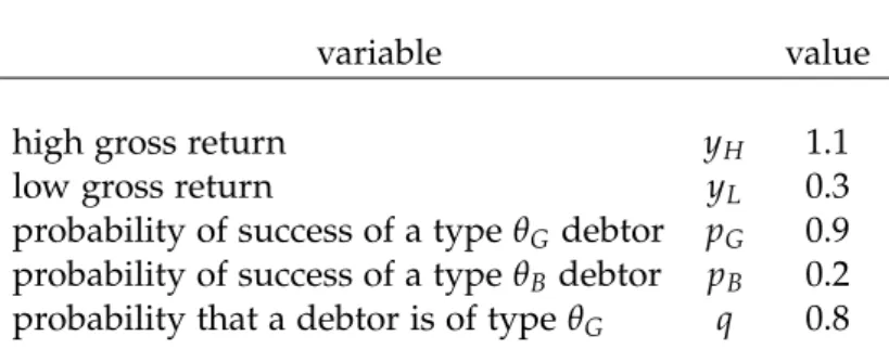
Starting for these values for the parameters of our game, we compare equilibrium outco-mes for different values of the parameters that characterize the legal environment. For each possible7value ofφandλ, we compute the profits of the creditor and of each type of debtor, as
well as the equity value, debt value and firm value. We also analyse how the loss due to ineffi-ciency change with respect to the value of these parameters. And finally, we compare the level of inefficiency in a pro-liquidation legal environment (ρ = 1) to that of a pro-reorganization legal environment. Figures1.2and1.3display these results.
7We restrict our attention to those parameter values for which liquidating the firm of typeθ=θ
Gis inefficient,
10
Figura 1.2: Expected payoffs in bankruptcy and loss due to inefficiency
This figure shows the expected payoffs of creditors and debtors (of both types) before the signaling game, as functions of two parameters of the economy derived from the legal environment: the liquidation costφ, and the creditor’s share of the firm’s liquidation value,λ.
Figure 1.2 brings the profits of the creditor, borrowers of type θG and θB, and the value
of losses due to inefficiency, all as functions of the liquidation costφand the creditor’s share of the project’s liquidation value λ. In the upper left corner, the graph shows the expected payoff of creditors, as the debtor firm enters reorganization. Notice that, as expected, as the creditor’s liquidation share increases, so does his expected profit. This is true even outside the pro-liquidation situation, because the in reorganization procedure of our model creditors retain the option of refusing to accept the offer made to them. Refusal leads to liquidation, and the creditor’s payoff in liquidation increases with λ. As the creditor’s outside option increases, so does the equilibrium offer debtors make.
In addition, for those values of φandλ that induce a separating equilibrium, the debtor of type θG must make an offer that is higher than the one he would make under symmetric
Figura 1.3: Debt and equity; equilibria of the renegotiation subgame
This figure shows the ex-ante expected profits of creditors and debtors, at the initial stage, as functions of two parameters of the economy derived from the legal environment: the liquidation costφ, and the creditor’s share of the firm’s liquidation value,λ. It also shows the equilibrium that arises in the signaling subgame, as function of
the same parameters.
This will translate into a lower interest rateR, as we can see in the top left corner of Figure 1.3. Axis are reversed, to facilitate observation. For high values ofφandλ– the same values that maximize the creditor’s payoff – we see the lowest interest rates.
Similarly, debtors’ expected payoffs grow with their share of the liquidation value(1−λ)
and with the liquidation value itself (φ), as we can see from the upper right and bottom left graphs in Figure 1.2). However, when we see the effect ofλ andφ on equity, we notice that those parameter values that induce a separating equilibrium, equity value will be increasing in λ. This occurs because, even though debtors’ payoffs in bankruptcy decrease with the creditor’s liquidation share, the effect on interest rates is even bigger. The decrease in interest rate affect equity, inasmuch as it increases the residual value of shareholders. Thus, in this case, a pro-creditor feature will actually have beneficialex-anteeffects for the debtor.
Finally, the bottom right graph of Figure 1.2shows the inefficiency losses in equilibrium. Since most values ofλandφproduce a separating equilibrium in our example, for most legal environments we would have an efficient outcome; only pooling equilibria, that arise for low values of φ, would give rise to inefficient outcomes, as one can see from Figure 1.3, in the bottom right graph.
Notice that, starting around φ = 0.8, the interval of values of λ that produce inefficient outcomes grows asφdecreases. Aroundφ=0.4, no matter how high is the debtor’s share in liquidation, the debtor of typeθB will find it profitable to impersonate the debtor of typeθG.
12
1.4 Empirical considerations
The discussion in the previous section highlights an important result, often ignored by the empirical literature on optimal bankruptcy law design: the outcome of a combination of legal features is not equal to the sum of their individual effects.
Moreover, credit market development is not a monotonic function of creditor protection. In our setup, when we compare two legal environments from the example in the previous section, (ρ = 1,λ = 1,φ > 0.8) and (ρ = 0,λ = 1,φ > 0.8), we find that the latter, although
less pro-creditor by the standards in the literature, results in higher creditor payoffs and lower interest rates.
The extent to which creditor protection actually affects equity and debt is mostly an em-pirical question, but one with no easy answer. The first issue that arises is how we can in fact measure creditor protection. Since the seminal works ofLa Porta et al.(1997,1998), their creditor rights index has been widely used as a measure of creditor protection for different legal environments. Their index is the sum of four qualitative binary variables that indicate the presence of each of the following legal features in each country for which it is computed:
1. No automatic stay on assets: some countries grant firms under court-supervised reor-ganization an automatic injunction protecting them from secured creditors that seek to seize the debt collateral. This variable is codified as one for countries that deny debtor firms such injunction.
2. Secured creditors come first in the event of liquidation: indicates if creditors with secured claims come first in the absolute priority rule that ordinates the distribution of the proceedings of the firm liquidation.
3. Managers of firms under reorganization can be removed at creditors discretion: indi-cates if creditors can remove managers they consider unfit to remain in charge of the firm under reorganization.
4. Reorganization is restricted: indicates if financially distressed firms seeking reorgani-zation must meet pre-determined conditions (such as creditors consent, or agree to a minimum level of dividends) to go into reorganization.
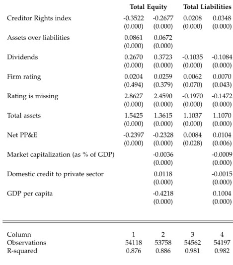
There is a large empirical literature that uses theLa Porta et al.(1997,1998) index to infer the correlation between creditor protection and various credit-related variables. This is done by including the creditor rights index as explanatory variable in OLS regressions to try to capture how it correlates to the regressand. Bae and Goyal (2009), Pistor et al. (2000), Qian and Strahan(2007) andDjankov et al.(2007) are a few papers that employ this method.
An often ignored problem with this approach is that it treats all legal environments with the same number of legal features – among those present in the index – as if they were the same. For example, a country in which creditors of insolvent firms come first in liquidation, but with automatic stay on assets and without managerial removal in reorganization or res-trictions to filing for reorganization is treated the same as a country, for instance, with only managerial removal and no other of the aforementioned legal features. To both of these coun-tries would be assigned the value “1"to describe how pro-creditor they are, in the scale of “0"to “4"that comprises the possible values that the index can take.
So, although the index can take only five different values, the combination of its compo-nents can potentially give rise to 24 = 16 different legal environments. Part of this problem
assigned the value of “1“; four assigned the value of “3"; and six assigned the value of “2” (see Table1.2).
In addition, including the sum of several binary variables as one single regressor con-founds their individual effects. Because of this, the regression might produce positive corre-lation with the index even though, for example, one of the index components is negatively correlated with the dependent variable.
Moreover, the linear model specification is not capable of answering questions regarding the optimal level of creditor protection. When we add the index as regressor, the estimated coefficient yields the correlation between the index and the regressand. It is not possible to obtain from the estimates a response for whether the data actually supports the existence of an intermediate optimal level of creditor protection or not. A positive correlation can be consistent with both a monotonic relation between the index and the variable of interest and a nonmonotonic one.
Both of these arguments are illustrated by Figure1.4. It displays the value of the intercepts in fifteen OLS regressions of, respectively, equity, debt, variance of equity, equity-to-liabilities ratio and firm value. All regressions have as covariates firm-specific control variables. Each regression was ran for a different subset from the firms in our sample, such that each data subset contains only observations for firms subject to the same legal environment. All but one possible combinations of the index components are represented. Notice that the correlation these values are not always increasing with the index value. These results show that it does not suffice to know the value of the index; it is also important to know which are the components whose presence in the legal environment yield such value.
Thus, it is not clear that a higher number of pro-creditor features would always be strictly preferred, by either debtors or creditors, to fewer pro-creditor features. It may be the case that creditors would prefer a legal environment with only, say, absolute priority in liquidation, to another with only restriction on filing for reorganization and managerial removal. If this is the case, the number of pro-creditor properties in a particular environment is less important than the pro-creditor properties themselves.
The policy evaluation approach
Instead of estimating an average correlation of the index against some variable of interest, a more informative approach could try to capture the marginal effect of these properties. For example, estimating the effect of adding automatic stay to each of the legal environments in which it is absent.
Some of the aforementioned problems with the typical approach could be diminished – some even solved – by employing methods borrowed from the treatment effects literature.8 So,
if we denote byΩ={ω1,ω2,· · · ,ω16}the set of possible legal environments – as described by
the combinations of the creditor rights index components in Table1.2– each legal environment can be thought of as a treatment. So, for firmiwe could write equity (Eit) and debt (Dit) in
periodt, under the treatmentωj ∈Ωas:
Eit(ωj) = fi(Xit) +βi(ωj) +uit (1.14)
Dit(ωj) = gi(Xit) +γi(ωj) +υit (1.15)
in whichXit account for observable variables that affect equity and debt, and uit and υit are
zero-mean terms.
14 Figura 1.4: OLS regression intercepts
Total Equity Total Liabilities Variance of Equity
0 1 2 3 4
20 40 60
creditor protection index
regr
ession
inter
cept
0 1 2 3 4
13 13.5 14 14.5 15
creditor protection index
regr
ession
inter
cept
0 1 2 3 4
0 50 100
creditor protection index
regr
ession
inter
cept
Equity/Liabilities Firm Value
0 1 2 3 4
10 20
creditor protection index
regr
ession
inter
cept
0 1 2 3 4
0 20 40
creditor protection index
regr
ession
inter
In an ideal world, in which we can observe the same firm under different legal regimes at the same time, we could simply subtract the value of our variable of interest for the same firm at the same time, under these two different regimes. Therefore, to obtain the effect of switching from a given legal systemωj to a systemωk we could simply compare our outcome
variables under these two different regimes to obtain the individual level treatment effects:
γi(ωk)−γi(ωj) = Dit(ωk)−Dit(ωj) (1.16)
βi(ωk)−βi(ωj) = Eit(ωk)−Eit(ωj) for ωj,ωk ∈Ω (1.17)
It follows, therefore, that if we consider the firm value to be the sum of both equity and debt, than the impact on the value of the firm of switching legal regimes would be the sum of the effects over these two variables:
Vit(ωk)−Vit(ωj) = [βi(ωk)−βi(ωj)] + [γi(ωk)−γi(ωj)] (1.18)
This straightforward approach, however, is not feasible. At any point in time, we only observe one out of the sixteen possible outcomes, since each firm operates under only one legal regime. This is the so-called “evaluation problem”, that makes it impossible to identify the individual level treatment effect for any given firm.
The typical alternative is to focus on some form of the marginal treatment effect, such as the Average Treatment Effect (ATE). As a matter of fact, if we expect all firms to be equally affected by the change in the law, the ATE is equal to the firm level treatment effect, for all firms, and we would lose no information by focusing on it. However, homogeneity of treat-ment effects does not seem to be a reasonable assumption. The choice of legal system affects the disposition of firm assets following default – and, hence, theex postpayoff of equityholders
and debtholders. So, firms with more sellable and valuable assets should be more affected by the choice of legal regime than firms with less valuable assets. In addition, the default probabilities themselves are affected by the regime choice, since the latter impacts firm risk taking. So, firms different in aspects such as default probability or liquidation value are ex-pected to be also different with respect to the impact of bankruptcy-related legal changes. In summary, different firms (with different characteristics) will be affected differently by the treatment. Hence, assuming the effect of legal change to be homogenous would probably be a stretch.
Moreover, there is also the issue of universal coverage. Since, at any point in time, all firms within any given country are subject to the same legal regime – and compliance with the legal regime is most often mandatory9 – we are left with no natural candidate for control group.
Estimating equations (1.14) and (1.15) with cross-country panel data would probably yield biased results, since the zero-mean assumption for the unobservable terms in these equations would no longer be reasonable.
The approach we take in this chapter to circumvent this problem and estimate the average treatment effect consists of finding a substitute for the ideal control group. Similarly to Bell et al.(1999) andAraujo et al.(2012a), we estimate this parameter by using the trend-adjusted difference-in-differences estimator, in which firms from countries that did not experience a change in the legal system are used as control group.
The underlying identification assumption is that we can decompose the unobservable terms in (1.14) and (1.15) into an incidental parameter, a macro effect whose impact differs from firm to firm, and a firm-level time varying uncorrelated effect:
uit= ηi+δimt+ǫit (1.19)
υit =µi+γint+ξit (1.20)
such thatE[ξ
it] =E[ǫit] =0.
16
Tabela 1.2: All possible legal environments
This table brings all possible combinations of the legal features present in the La Porta et al.(1997,1998) creditor rights index. Each combination describes one possible legal environment.
Legal System
Creditors Rights
Index
Does not allow for automatic
stay
Secured Creditors come First in Liquidation
Managers are Removed in Reorganization
Restrictions in filing for Reorganization
1 0 False False False False
2 1 True False False False
3 1 False True False False
4 1 False False True False
5 1 False False False True
6 2 True True False False
7 2 True False True False
8 2 True False False True
9 2 False True True False
10 2 False True False True
11 2 False False True True
12 3 True True True False
13 3 True True False True
14 3 True False True True
15 3 False True True True
This hypothesis makes our model general enough to account for different macro trends, an important characteristic since we using firms from several different countries to estimate the average treatment effect.
1.5 Estimation
In this section we present the estimation data and results. We run two sets of regressions. The first set replicates the method commonly employed in the Law and Finance literature, by adding the creditor rights index in the right-hand side of standard linear regression models along firm-specific controls and, in some cases, macro variables. The second set estimates the average treatment effect on the treated (ATT) parameter, taking advantage of institutional changes in various countries to identify the average effect of: i) an increase in the creditor’s protection index by one unity; ii) denying debtor firms in reorganization the possibility of an automatic stay on their assets; and iii) granting creditors of firms in reorganization the power of removing firm management.
1.5.1 Data
The estimates reported in this chapter were computed using data from Compustat Global. This is the source of firm-specific data that comes from financial statements, such as dividends paid, total assets, total liabilities, net PP&E (plant, property and equipment) and firm industry sector. Sectors correspond to the Standard Industry Classification Codes (SIC codes), that span from zero to nine. As is common in the literature, we exclude from our sample firms with SIC codes six (financial companies) and nine (government).
The equity value is calculated at the last day of each year, by multiplying the closing price of one share of firm stock by the number of shares outstanding. Data on stock prices come from Compustat Global, and is reported in the currency of each country. We use exchange rate quotes from the same trading day to convert equity prices to the same currency. For the variance of firm equity in any given fiscal year, we use the stock quotes of the twelve months in that year.
We work with a panel data of firms from 55 different countries, with time span ranging from 1993 to 2003
In some model specifications, we also include macro variables – such as GDP per capita, market capitalization (as a percentage of the country’s GDP) and the domestic credit to the private sector within the country – as controls. These information come from the World Bank. Information on legal environments and their changes come fromDjankov et al.(2007).
1.5.2 Results
Cross-country OLS regressions
We run basically two different specifications of the reduced model: one with the aforementi-oned macroeconomic variables, and the other without.
Our results are displayed in tables (1.4) to (1.13).
18
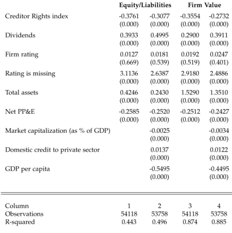
index. All these results are highly significant. We do not find significant estimates on the equity-to-liabilities ratio.
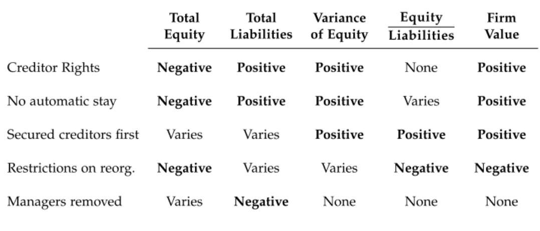
Tabela 1.3: Summary of results
This table presents a summary of the results. the results of trend-adjusted difference-in-difference estimates, having as dependent variables the logarithm of the firm’s total equity, its total liabilities, the equity variance, the ratio and the sum of these two variables. The whose average effect on the treated we wish to estimate is a legal change that increases the Creditor Rights index, introduced by La Porta et al.(1997, 1998). We also control for firm-level characteristics. Only point estimates and p-values (in parentheses) are reported.
Panel A: Correlations (Tables1.4to1.13)
Total Equity
Total Liabilities
Variance of Equity
Equity Liabilities
Firm Value
Creditor Rights Negative Positive Positive None Positive
No automatic stay Negative Positive Positive Varies Positive
Secured creditors first Varies Varies Positive Positive Positive
Restrictions on reorg. Negative Varies Varies Negative Negative
Managers removed Varies Negative None None None
Panel B: Average treatment effect on the treated (Tables1.14to1.16)
Total
Equity LiabilitiesTotal of EquityVariance
Equity Liabilities
Firm Value
Increase in CR Index effectNo Positiveeffect effectNo effectNo effectNo
No Automatic Stay Negativeeffect effectNo effectNo Negativeeffect Negativeeffect
Managers removed No effect
No effect
No effect
No effect
No effect
We also run regressions with the components of the index added separately as regressors. In tables (1.6) to (1.13), we explore how the presence of each individual characteristic relates to our variables of interest.
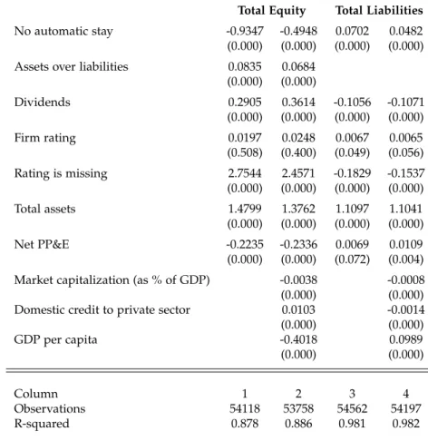
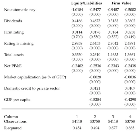
Tables (1.6) and (1.7) displays the results regarding automatic stay on assets. Similarly to our first results, we find the absence of automatic stay to be positively correlated to the firm’s total liabilities and value, but negatively correlated to equity. Yhe variance of equity also increases when no automatic stay is in place. Estimates for the effect on equity-to-liabilities ratio change, depending on the model specification.
Regarding the countries that restrict the reorganization petitions, we find mostly all cor-relation estimates to be negative. Total equity, the variance of equity, firm value and the equity-to-liabilities ratio, all these variables tend to decrease when such restrictions are in place. The estimates appear in Tables (1.8) and (1.9). Results on liabilities, however, are mi-xed. In one specification (the one without the macro variables as controls) we find a negative correlation, but once we add these controls the correlation becomes positive.
Finally, for countries in which creditors can remove managers of firms in reorganization, we find mixed results for firm equity and the equity-to-liabilities ratio. No significant estima-tes are produced for firm value, but total liabilities and the variance of equity both increase. Tables (1.12) and (1.13) are the ones that display the regression results.
Average treatment effect on the treated
The estimates reported in tables (1.4) to (1.13) are all potentially problematic, since many factors may be at play in cross-country regressions. Some of the estimates turn from negative to positive, or vice-versa, depending on the number of variables in the right-hand side of the equation. This behavior, although undesirable, is common in cross-country regressions that focus on correlations.
The next subsection presents the estimation results of for the average treatment effects on the treated, an approach that relies on better identification assumptions.
We take advantage of the institutional changes that took place in some countries between 1993 and 2003. This variability helps on evaluating how, for example, an exogenous increase in the creditor rights index affects, on average, our variables of interest. We also examine the effect of some of the index individual components on the same variables. However, for lack of data on some countries, for now we only have estimates for automatic stay and managerial removal. The estimates we do have are for the average treatment effect on the treated (ATT), identified through the strategy described in the previous section and estimated by a trend-adjusted difference-in-differences estimator. Tables (1.14) to (1.16) display the results of these estimates.
The first of these tables brings the estimation results for the ATT when the “treatment” is an exogenous increase by one unit in the value of the creditor rights index. Notice that almost all results are inconclusive, since four out of the five estimates are not statistically significant. All of them are somehow related to firm equity: total equity, variance of equity, equity-to-liabilities ratio and firm value.
The only regression that yields a significant estimate is the one for the firm’s total liabili-ties. Moreover, the point estimate itself is consistent with the empirical literature and with a positive impact of creditor protection in the supply of debt.
The more interesting results are the ones we present in the last two tables. When evaluating the effect of the individual index components, we find that index confounds their individual effects. Table 1.15brings the results for the effect of automatic stay on assets. We find that denying debtor firms the possibility of an automatic stay reduces firm equity, firm value and the equity-to-liabilities ratio. We find no significant effect on total liabilities, but we do find an increase in the variance of equity with a p-value of 0.03.
Table1.16, on the other hand, find somewhat different results for removing managers from firms in reorganization. The effect of granting creditors that power seems to be positive for firm debt, but we find no significant result on any other variable.
This is the first of the three main arguments in favor of bankruptcy laws with Chapter 11-like provisions that we revisit in this chapter.
20
for political reasons, since Congress was keen to granting firms a second chance. In Argentina, Congress changed the law during the 2002 crisis because lawmakers believed banks were taking over too many firms. Similarly, Mexican Judiciary rejected the law that was too pro-creditor, and created a bureaucratic law that included “visitadores” and “conciliadores”. Thus, it might be preferable to seek a less stringent but politically feasible bankruptcy law, with less uncertain enforcement, than seeking a more severe law with higher risk of being either defeated in Congress or ignored by the Judiciary.
Finally, court-supervised reorganizations might also make sense from a short-run macro-economic standpoint. Allowing firms a grace period during which they can organize their financials might help mitigate crisis and avoid fire sales. Laws with Chapter 11-like provisi-ons are most strongly tested during periods of crisis – specially credit crisis, when financing adverse shocks becomes even more difficult. In times like these, the number of bankrupt-cies usually increase, so bankruptcy laws can play an important role in alleviating crisis and accelerating turnarounds. In section 4, we bring some data on this.
1.6 Concluding Remarks
In this chapter we investigate how different legal features – most notably, automatic stay on assets and managerial removal during reorganizations – affect corporate debtors and credi-tors. We propose an empirical approach that differs from the one usually taken in the Law and Finance literature and find results that are also different. Our results are motivated by an adverse selection model in which deviations from the “Absolute Priority Rule” may incre-ase welfare. In our setup, giving firms a second chance, while preserving creditors rights in liquidation, can be described by a signaling mechanism capable of driving inefficient firms out of the market, while preserving the value of firms with high probability of success. This mechanism – roughly matching Chapter 11 reorganization – results in lower interest rates, higher creditor payoffs and higher equity values, for legal environments in which a separa-ting Bayesian equilibrium emerges. Our results are also in line with the general equilibrium with incomplete markets and default models – that prescribe an intermediate level of default penalty for the development of credit markets – as well as several other models in partial equilibrium setups.