Comparative advantage, heterogeneous firms and variable mark-ups

FUNDAC

¸ ˜

AO GETULIO VARGAS

ESCOLA DE P ´

OS-GRADUAC

¸ ˜

AO EM

ECONOMIA

Rafael Amaral Ornelas

Comparative Advantage, Heterogeneous Firms and

Variable Mark-ups

Rafael Amaral Ornelas

Comparative Advantage, Heterogeneous Firms and

Variable Mark-ups

Disserta¸c˜ao submetida a Escola de P´os-Gradua¸c˜ao em Economia como requisito par-cial para a obten¸c˜ao do grau de Mestre em Economia.

´

Area de Concentra¸c˜ao: Com´ercio Internacional

Orientador: Afonso Arinos de Mello Franco Neto

Ficha catalográfica elaborada pela Biblioteca Mario Henrique Simonsen/FGV

Ornelas, Rafael Amaral

Comparative advantage, heterogeneous firms and variable mark-ups / Rafael Amaral Ornelas. - 2014.

45 f.

Dissertação (mestrado) - Fundação Getulio Vargas, Escola de Pós-Graduação em Economia.

Orientador: Afonso Arinos de Mello Franco Neto. Inclui bibliografia.

1. Comércio internacional. 2. Vantagem comparativa (Comércio). I. Franco Neto, Afonso Arinos de Mello. II. Fundação Getulio Vargas. Escola de Pós- Graduação em Economia. III. Título.

Abstract

We develop a model of comparative advantage with monopolistic competition, that incorporates heterogeneous firms and endogenous mark-ups. We analyse how these features vary across countries with different factor endowments, and across markets of different size. In this model we can obtain trade gains via two channels. First, when we open the economy, most productive firms start to export their product, then, they demand more producing factors and wages rises, thus, those firms that are less productive will be forced to stop to produce. Second channel is via endogenous ups, when we open the economy, the competition gets “tougher”, then, mark-ups falls, thus, those firms that are less productive will stop to produce. We also show that comparative advantage works as a “third channel” of trade gains, because, all trade gains results are magnified in comparative advantage industry of both countries. We also make a numerical exercise to see how endogenous variables of the model vary when trade costs fall.

Contents

1 Introduction 7

2 Closed Economy 9

2.1 Consumption . . . 10

2.2 Profit Maximizing Price . . . 11

2.3 Production . . . 11

2.4 Cutoff Productivity Levels . . . 12

2.5 Market Clearing . . . 14

3 Costly Trade 15 3.1 Cutoff Productivity Levels . . . 17

3.2 Market Clearing . . . 20

4 Results in the Costly Trade Equilibrium 21 5 Numerical Example 25 6 Conclusion 32 7 Appendix 36

List of Figures

2 Average productivity . . . 27

3 Average firm output . . . 28

4 Differences in comparative advantage . . . 28

5 Exporting probability . . . 29

6 Mass of firms (domestic varieties) . . . 29

7 Mass of entrants . . . 30

8 Welfare evaluation . . . 30

1

Introduction

Since Melitz (2003), many authors have used his model of heterogeneous firms as a start-ing point to their own models1_{. By using Melitz’s model, researchers could obtain results}

of trade gains by two channels. In one hand, as in Melitz (2003), trade induces competi-tion for scarce labour resources as real wages are bid up by the relatively more productive firms who expand production to serve export markets. Bernard et al. (2007) obtained trade gains by this channel, but their model also focus in comparative advantage, which magnifies trade gains at comparative advantage industry. On the other hand, in Melitz and Ottaviano (2008) and in Rodriguez-Lopez (2011), import competition increases com-petition in the domestic product market, shifting up residual demand price elasticities for all firms at any given demand level. However, increased factor market competition plays no role in those models.

The differences in the origin of trade gains between those models is in the utility of the consumers. The first group, which follows Melitz (2003), uses CES utility and it does not permit price elasticity to vary. When it does vary we have endogenous mark-ups, what permits trade gains via the second channel, which is done by the second group. The main contribution of this paper is to put these two channels together into a unique framework. Thus, our model permits trade gains via both channels. We analyse international trade in an environment that allows endogenous mark-ups and yet have two industries and comparative advantage effects. We find in one model many results that were before found separately.

We develop a monopolistic competitive model of trade with heterogeneous firms, two industries, and endogenous mark-ups. This environment allows our model to obtain trade gains by both channels already mentioned. Firm heterogeneity is introduced similarly to Melitz (2003), by productivity differences. We introduce endogenous mark-ups using translog expenditure functions in the demand side. This technique was introduced in Feenstra (2003), used in Arkolakis et al. (2010), and in Rodr´ıguez-L´opez (2011). Translog expenditure functions are useful because it permit price elasticity to vary, differently from CES, although, preference still homothetic. We follow basically three papers, Bernard, Redding and Schott (2007), Melitz and Ottaviano (2008) and Rodriguez-Lopez (2011).

As in Melitz and Ottaviano (2008), in our model, market size and trade affect the toughness of competition in a market, which then feeds back into the selection of hetero-geneous producers and exporters in that market2_{. The fact that we have two industries}

also influences this selection. We are able to find similar results to those found in Bernard, Redding and Schott (2007) with the advantage that in our model the mark-ups are free to vary. Although, our model remains tractable.

First we develop a closed-economy version of our model. As in Melitz and Ottaviano (2008), differently from Melitz (2003), the market size induces important changes in the equilibrium distribution of firms and their performance measures. Larger markets require higher productivity cutoffs. Larger markets also has firmsthat are larger and earn higher profits. We then present the open-economy in costly trade.

When the economy moves from autarky to costly trade we show that larger markets still exhibit larger and more productive firms, lower prices, and lower mark-ups. We also

1

Other internatinal trade models also incorporate heterogeneous firms, Bernard et al. (2003); Helpman et al. (2004); Yeaple (2005).

2

find the same results found in Bernard, Redding and Schott (2007). When countries move simultaneously from autarky to costly trade, firms export opportunities increase. It promotes greater entry from the competitive fringe. However, the mass of domestic producers gets lower in both countries. Most productive firms start to sell at the ex-port market. The proex-portion of firms exex-porting will be higher in comparative industry. The productivity cut off necessary to produce increases and the most productive firms start to export, inducing aggregate productivity level in each industry to grow3_{. This}

result is higher in comparative advantage industry and intensifies its ex ante compara-tive advantage, which raises trade gains. After opening the market, all firms set smaller mark-ups, an effect that is higher in firms from comparative advantage industry. How-ever, average mark-ups in both industries do not change. These findings contrast with the homogeneous-firm imperfect competition model of Helpman and Krugman (1987)4_,

where industry productivity remains constant and, depending on the value of fixed and variable trade costs, either all or no firms export, when there is trade liberalization.

When we take a look into distributional implications, our framework is able to find the famous Stoper-Samuelson result, but also, there is an other effect. In consequence of aggregate productivity growth, average price of the variety is reduced in each industry and thereby elevates real income of both factors. Thus, even if the real wage of the scarce factor falls during opening trade, its decline is less than it would be in a Neoclassical setting. The falling of all mark-ups of those remaining firms reduces the price for each variety, but, once average mark-up is constant, there is no effect on average prices.

As in Bernard, Redding and Schott (2007), our approach also generates predictions about the impact of trade liberalization on job turnover that are different from those obtained in a Neoclassical model. We show that a reduction in trade barriers encourages simultaneous job creation and job destruction in all industries, but gross and net job creation vary with country and industry characteristics.

Differently from Bernard et al. (2007), we have closed functions for all endogenous variables. Using these facility of the model, we constructed a numerical exercise, where we calibrate our model to an symmetric environment and vary trade costs, then we analyse how endogenous variables vary. In this numerical exercise, we calculate a weighted average mark-up, thus it vary when trade costs change. We found that when competition gets “tougher”, weighted average mark-up fall, as average mark-up in Melitz and Ottaviano (2008).

All models using endogenous mark-ups generate the equilibrium property that more productive firms charge higher mark-ups. Bernard et al. (2003) also incorporate firm heterogeneity and endogenous mark-ups in their model. However, the distribution of mark-ups is invariant to country characteristics and to geographic barriers. Melitz and Ottaviano (2008) develop a non-degenerate distribution of mark-ups, that depends on country characteristics and on geographic barriers, but they have only one industry and there are no effects from comparative advantage. They analyse asymmetric trade liber-alization scenarios. Rodriguez-Lopez (2011) presents a sticky-wage model of exchange rate pass-through with heterogeneous producers and endogenous mark-ups. Arkolakis, Costinot and Rodr´ıguez-Clare (2010) provide a simple example with Translog

Expendi-3

Empirical studies strongly confirm these selection effects of trade (only most productive firms export). For example, see Clerides et al. (1998); Bernard and Bradford Jensen (1999); Aw et al. (2000); Pavcnik (2002); and Bernard et al. (2006).

4

ture Functions and Pareto distribution of firm-level productivity, they have an environ-ment close to ours, where mark-ups vary. However, they also have only one industry in their model. In this paper we focus on the effects that variable mark-ups cause in an economy when it moves from closed to open economy. Not only has our model two industries, but we also analyse the effect of endogenous mark-ups in this environment with advantage comparative. Our approach permits us to find closed-solutions for all endogenous variables of the equilibrium.

Zhelobodko et al. (2012) propose a model of monopolistic competition with additive preferences and variable marginal costs. They use the concept of “relative love for variety” (RLV) to provide a full characterization of the free-entry equilibrium. In their work they show that when we use CES utility, as the elasticity of substitution, RLV will also be constant, it is a specific case where prices and mark-ups are not affected by firm entry and market size, but they are interested in those cases where RLV are free to vary. Our model goes in this direction and our results are corroborate by those results from Zhelobodko et al. (2012) when RLV increases.

In Arkolakis et al. (2012), the authors analyse if micro-level data have had a profound influence on research in international trade over the last years. They found that, although models have became more detailed, the amount of welfare gains did not change so much when compared with those obtained by simpler models, like the Armington model. They made some assumptions like CES utility that we do not use in our model, but Arkolakis et al. (2010) shows that the main result holds in a model similar to that used in Rodr´ıguez-L´opez (2011). However, in Arkolakis, Costinot, Donaldson, and Rodr´ıguez-Clare (2012), the authors study the pro-competitive effects of international trade in models that allow variable mark-ups, including models with the continuous translog expenditure function. They find out that gains from trade liberalization are weakly lower than those predicted by the models with constant mark-ups considered in Arkolakis et al. (2012). They argu-ment that “there is incomplete pass-through of changes in marginal costs from firm to consumers”.

Finally, our model could be a more useful benchmark than the existing theory for predicting the pattern of trade. The Neoclassical standard Heckscher-Ohlin-Vanek model presents poor empirical performance, because it does not capture the existence of trading costs, the factor price inequality, and the variation in technology and productivity across countries5_.

The remainder of the paper is structured as follows. Section 2 introduces the model for closed economy. Section 3 expand the model to a costly trade economy. In section 4, we present the results that we find when the economy moves from autarky to costly trade. Section 5 present a numerical exercise, and section 6 concludes the study.

2

Closed Economy

In this section we will solve the model for the case that the economy is closed, so there are no exporters in this section. Consider an economy with L consumers.

5

2.1

Consumption

The representative consumer’s utility in the upper tier is given by a Cobb-Douglas utility function, in the lower tier the utility is given by the continuous translog expenditure function as in Rodriguez-Lopez (2011). Preferences are defined for a continuum of dif-ferentiated goods, in each industry, h = {x, y}, set of goods, Ωh. Each set includes the

total number of actual, and potential (not yet invented) goods and has measure of ˜Nh.

Let Ω′

h, with measure Nh, be the subset of Ωh that contains the set of goods that are

available for purchase in the economy. Utility level is U, and Ph is the price index for

industry h, then the expenditure function of the representative consumer is given by:

lnE = lnU+αxlnPx+αylnPy.

Where αx+αy = 1, and;

lnPh =

1 2γhNh

+ 1

Nh

Z

i∈Ω′ h

lnpihdi+ γh

2Nh

Z

i∈Ω′ h

Z

j∈Ω′ h

lnpi(lnpj−lnpi)djdi. (1)

Where γh > 0 indicates the degree of substitutability between goods: with larger

values of γh implying higher substitutability between goods in that industry (low

differ-entiation). Consumers exhibit “love of variety”: when the set of goods in the economy,

Nh, is larger, the expenditure necessary to achieve utility U is lower.

In this economy we have two kind of agents, skilled workers and unskilled workers, each type of worker will offer one unit of labour. The size of the economy is given by

L=Ls+Lu. wk is the wage earned by the worker, k ={s, u}. The aggregate income is

given by I =wsLs+wuLu.

The share sih of good i from industry h in the expenditure of the consumer using

Shephard’s lemma is given by;

sih=

∂lnE

∂lnpih

=αh

1

Nh

+ γh

Nh

Z

j∈Ω′ h

lnpjhdj−γhlnpih

!

.

Note that when sih = 0 we have that pih = ˆph, where ˆph = exp

1

γhNh +lnpgh

is the chock-off price, that is the highest price that a firm i can charge in industry h, and sell anything and, lnpgh = _N1

h

R

j∈Ω′_hlnpjhdj is the average log price. Then, sih =αhγhln

ˆ ph pih . (2)

Using 2 we can write the quantity demanded of a good i in industry h.

qih=γhln

ˆ

ph pih

αhI pih

.

2.2

Profit Maximizing Price

Assuming a constant marginal cost for each firm i, each firm will solve the maximization problem:

maxpihpihqih−cihqih.

The solution is pih = [1 +ln(ˆph/pih)]cih. Note that,

pih cih

= 1 + ln

b

ph cih

cih pih

,

pih cih

epihcih ₌ pbh cih

e,

pih cih

= W

b

ph cih e

.

Where W(z) is the Lambert function defined as the inverse of x = zez _{for x > 0}6_.

Thus;

pih=W

ˆ

ph cih

e

cih. (3)

Using 3 we define the mark-up of firm i in industry h as

µih≡ W

ˆ

ph cih

e

−1. (4)

Then,

pih= (1 +µih)cih, (5)

lnpih=lnpˆh −µih, (6)

sih=γhµih. (7)

2.3

Production

Each industryh ={x, y} uses skill and unskilled labour with different intensities. Indus-try x is intensive in skilled labour and industry y in unskilled labour, to that βx > βy.

Marginal cost of production of each firm in each industry is

ch(ϕ) =

(ws)βh(wu)1−βh

ϕ .

In this economy, production will follow Melitz (2003) and Bernard, Redding and Schott (2007). Each firm will invest a sunk costfE(ws)βh(wu)1−βh, to draw a productivity ϕ from a distribution g(ϕ) to ϕ ∈ [ϕ,+∞) seeking to produce in industry h, so that production and investment to enter the industry imply factors in the same proportion, given wages. Price in the domestic market is then given by:

6

ph(ϕ) = (1 +µh(ϕ))

(ws)βh(wu)1−βh

ϕ . (8)

The mark-up is:

µh(ϕ) =W



 pˆh

(ws)βh(wu)1−βh ϕ

e



−1. (9)

Output, yh(ϕ), revenue, rh(ϕ), and the profit, πh(ϕ), of each firm can be calculated

substituting optimum price (5) in the demand (2).

yh(ϕ) = γhIh ch(ϕ)

µh(ϕ)

1 +µh(ϕ)

,

rh(ϕ) =ph(ϕ)yh(ϕ) = γhIhµh(ϕ),

πh(ϕ) =γhIh

µh(ϕ)2

1 +µh(ϕ) .

More productive firms set lower prices and earn higher revenues and profits and set higher mark-ups.

2.4

Cutoff Productivity Levels

The cutoff ϕh determines which firms will produce in each industry. Firms only produce

if their profit is non negative, that is, ifϕ ≥ϕh where ϕh = inf{ϕ :µh(ϕ)>0}. Thus;

ϕh =

(ws)βh(wu)1−βh

ˆ

ph

.

The cutoff productivity is higher the lower is the chock-off price and the higher are input costs.

To proceed further we adopt the Pareto distribution for productivities, as in Melitz and Ottaviano (2008) with density function for ϕ∈[ϕ,∞] and k ≥1.

g(ϕ) = kϕ

k

ϕk+1,

and distribution function,

G(ϕ) = 1−

_ϕ

ϕ

k

.

Thus, the distribution of those firms that draw a productivity ϕ high enough to be active in industry h is

g(ϕ|ϕ > ϕh) =

( _kϕk

h

ϕk+1; ifϕ > ϕh

0; otherwise

e

ϕh(ϕh) =

Z ∞

ϕh

ϕ kϕ

k h

ϕk+1dϕ=

k k−1ϕh.

Note that, we can write the mark-ups of the firms as a function of their productivity and the cutoff;

µh(ϕ, ϕh) =W

ϕ ϕh

e

−1.

Firms with higher productivities set higher mark-ups, but they are lower in industries with higher cutoffs.

Since the distribution ofϕ/ϕh is invariant under a Pareto distribution for productivity,

the average mark-up depend only on the parameter k of the distribution and so it is the same for both industries.

Z ∞

ϕh

µh(ϕ, ϕh) kϕk

h

ϕk+1dϕ=k

Z ∞

1

W(xe)−1

xk+1 dx=µe(k).

As in Melitz (2003), in every period each firm has a positive probability δ to have a bad shock and “die”. The value of the firm with productivity ϕ is

vh(ϕ) = max{0,Σ(1−δ)πh(ϕ)}

= max{0,πh(ϕ)

δ }

With free entry, the expected value of the firm should equal the sunk cost incurred to draw a productivity from g(ϕ). The ex-ante expected profit of the firm πe

h is given by: πeh =

Z ∞

ϕh

πh(ϕ)g(ϕ)dϕ= ψhIh

ϕk h

.

Where, ψh =γhχe(k)ϕk, and χ(k) = k

R∞

1

(W(xe)−1)2

W_(xe)xk+1dx, is a constant depending only

on parameter k.

The free entry condition is

πe h

δ =fE(ws) βh_(w

u)1

−βh_.

Thus,

ψhIh ϕk

h

=δfE(ws)βh(wu)1−βh. (10)

Using the FECs we can determine the cutoff productivity levels as functions only of parameters and wages;

ϕh =

ψhIh

δfE(ws)βh(wu)1−βh

1 k

. (11)

In the closed economy, larger market size, as measured by Ih, and a higher degree

of substitutability between the goods, γh, implies a higher cutoff productivity. Because

With the cutoffs determined and the definition for chock-off prices we can determine the mass of producing firms in each industry.

Proposition 2.1. The mass of available goods in each industry depends only on the substitutability among varieties;

Nh =

1

γh(ln ˆph−lngph)

= 1

γhµe(k)

. (12)

Proof. See Appendix.

The mass of available goods is larger in the industry with lowerγh. Number of varieties

is higher when they are less substitutable.

GivenNh, LetNphdenote the measure of the pool of existing firms in industryh, that

is the mass of firms that pay the sunk cost to draw a productivity. These firms in the pool can be producing or not, depending on their productivity ϕ and the productivity cutoff, ϕh. Since 1−G(ϕh) is the fraction of investors that became producing firms;

Nh = (1−G(ϕh))Nph =

_ϕ

ϕh

k

Nph.

In steady-state, we have that the following relation is valid:

Nph;t+1 = (1−δ)Nph;t+NEh;t+1.

Where NEh is the mass of entrant firms in industry h. In steady-state, we must have Nph;t+1 =Nph;t=Nph. Thus7,

δNph =NEh.

In conclusion, the mass of firms that “die” every period in each industry is equal the mass of entrants firms in the same industry.

2.5

Market Clearing

In this section we will use the marketing clearing conditions to determine the wage vector [ws, wu].

Revenue that a firm with productivity ϕ∈[ϕ,∞] in the industry h={x, y}earns in the domestic market is

rh(ϕ) = ph(ϕ)yh(ϕ) =γhIh

W

ϕ ϕh

e

−1

.

Let Rh be the total revenue of industry h={x, y}.

Rh =Nh

Z ∞

ϕh γhIh

W

ϕ ϕh

e

−1

kϕk h

ϕk+1dϕ

Using a change of variables, x = ϕ/ϕh, and the previous result for Nh and average

mark-up µ_e(k), we have that, 7

Rh =γhNhIhµe(k) =Ih. (13)

The total revenue of industry h is equal the total expending on varieties from that industry. FEC is used to show that all profit made in each industry will be spent paying labour employed in the entry technology for the same sector.

Proposition 2.2. Expenditures on entry investment employment are equal to profits in each sector.

NEhfE(ws)βh(wu)1

−βh _{= Π} h.

Proof. See Appendix.

Market clearing of labour market require thatLk =Lkx+Lky. WhereLkh =LDpkh+LEkh

and superscripts refer to workers employed in production and entry investment respec-tively. We can determine relative wages using labour demand and labour market clearing conditions.

Proposition 2.3. Equilibrium wages defined only on comparative advantage parameters.

wu ws

= 1−(αβx+ (1−α)βy) (αβx+ (1−α)βy)

Ls Lu .

Proof. See Appendix.

With wages determined, all the equilibrium for the closed economy can be described: Because average mark-up are constant and equal for both industries, the equilibrium relative wages reflect directly relative demand and supply facts, independently of intra industries competition.

3

Costly Trade

We extend the model for two countries, “Home Country” and “Foreign Country”’, that will be represented by an asterisk. Firms in each of the two industries, h = {x, y}, can sell in markets r = {D, X}, domestic market and export market. We adopt the standard Heckscher-Ohlin assumption that countries are identical in terms of preferences and technologies, but differ in terms of endowments. The Home Country is the skilled labour abundant country and the Foreign Country is the skilled labour scarce country, as described by their relative endowmentsLS/LU > LS

∗

/LU

∗

. Factors of production can move between industries within countries, but not across countries.

Costs to export are modelled as ice-berg costs. It is necessary to ship τh > 1 units

of the good for one unit to be delivered in the other country for consumption, we allow for different ice-berg costs to each industry h. As in Bernard et al. (2007) we show how these trade costs interact with comparative advantage to determine responses to trade liberalization that vary across firms, industries, and countries. Market size, factor intensity and factor abundance also play an important role in shaping within-industry reallocations of resources from less to more productive firms. But differently from Bernard et al. (2007), the equilibria in our model also have mark-ups heterogeneity.

In open economy, producing firms can sell in two different markets. They sell output

enough, it sells outputyXh(ϕ) to the Foreign Country by pricepXh(ϕ). Firms in Foreign

Country are in the same environment. In consequence of transportation costs, only the more productive firms will make profitable sales in the export market. That will define two different cutoffs productivities, one for firms selling exclusively in the domestic market market, and the other for exporters.

Since the markets are segmented8 _{and firms produce under constant marginal costs,}

they independently maximize profits earned from domestic and export sales. Using the results from before and taking account the transportation cost,τh, we have the following

mark-ups for domestic and export sales:

µDh(ϕ) ≡ W



 pˆh

(ws)βh(wu)1−βh ϕ

e



−1 =W

ϕ

ϕDh

e

−1,

µXh(ϕ) ≡ W



 pˆ∗h

τh(ws)

βh(wu)1−βh ϕ

e



−1 =W

ϕ

ϕXh

e

−1.

Other domestic and export firm variables can be written as functions of the respective cutoffs and mark-ups:

pDh(ϕ) = (1 +µDh(ϕ))

(ws)βh(wu)1−βh

ϕ ,

pXh(ϕ) = (1 +µXh(ϕ))τh

(ws)βh(wu)1−βh

ϕ ,

yDh =

γhIh ch(ϕ)

µDh(ϕ)

1 +µDh(ϕ)

,

yXh=

γhIh∗ τhch(ϕ)

µXh(ϕ)

1 +µXh(ϕ)

,

rDh(ϕ) = pDh(ϕ)yDh(ϕ) = γhIhµDh(ϕ),

rXh(ϕ) = pXh(ϕ)yXh(ϕ) = γhIh∗µXh(ϕ),

πDh(ϕ) =γhIh

µDh(ϕ)2

1 +µDh(ϕ) ,

πXh(ϕ) = γhI

∗

h

µXh(ϕ)2

1 +µXh(ϕ) .

8

3.1

Cutoff Productivity Levels

To determine the cutoffs productivity levels we use the fact that a firm will sell to a determinate market only if it draws a productivity high enough to turn in positive profits, that is: ϕrh =inf{ϕ:µrh(ϕ)>0}. Using the definitions for the demand chock-off price

in each market, ˆph and ˆp∗h,

ϕDh =

(ws)βh(wu)1−βh

ˆ

ph

,

ϕXh = τh

(ws)βh(wu)1−βh

ˆ p∗ h , ϕ∗ Dh =

(w∗

s)βh(w

∗

u)1

−βh

ˆ

p∗

h

,

ϕ∗

Xh = τh

(w∗

s)βh(w

∗

u)1

−βh

ˆ

ph

.

The cutoffs productivities for an industry in a market is the ratio between the factor basket cost in the country and the industry chock-off price in the market.

Under costly trade, there are four different cutoffs: each country has one cutoff to produce for domestic market and one cutoff to produce for foreign market.

These equations imply direct relations between the cutoffs productivity levels: for national and foreign firms competing in each country;

ϕ∗

Xh = τhζhϕDh, (14)

ϕXh = τh

1

ζh ϕ∗

Dh, (15)

where ζh =

h

(w∗

s)βh(wu∗)1−βh (ws)βh(wu)1−βh

i

is the relative price of foreign factor basket. And between the cutoff productivity level for each country’s firms competing in domestic and export markets;

ϕXh = ΛhϕDh, (16)

ϕ∗

Xh = Λ

∗

hϕ

∗

Dh. (17)

Where, Λh =τhpbh/bp∗h >1 and Λ

∗

h =τhpb∗h/pbh >1.

Where the inequalities ensure that there is selection of firms into domestic only and exporters in both industries9_.

Note that equations (16) and (17) establish a relation between the export cutoff productivity level and the domestic cutoff productivity level in different country markets. It says that trade barriers make trade harder for exports to break even relative to domestic producers. Equations (18) and (19) ensure that the cutoff to export is higher than the cutoff to domestically production, then we will have separation in the market, only most productivity firms will export. We can show that non-arbitrage conditions over prices are verified (Claim 3.1).

9

The average productivity level is the same linear function of the cutoff that we have already found for the closed economy;

e

ϕrh(ϕrh) =

Z ∞

ϕrh

ϕkϕ

k rh

ϕk+1dϕ=

k k−1ϕrh.

The average mark-up for exports is the same constant as the one for domestic sales,

e

µ(k).

The FEC still need πhe

δ =fE(ws) βh(w

u)1−βh, but now expected profits include export

profits;

πhe =π e Dh+π

e Xh.

Where,

πe

Dh =

ψhIh ϕk

rh ,

πe

Xh =

ψhIh∗ ϕk

rh .

As before, ψh = γhχe(k)ϕk, and χe(k) = k

R∞

1

(W(xe)−1)2

W(xe)xk+1dx, is a constant depending

only on parameter k.

The FECs are:

1

δ

ψhIh ϕk

Dh

+ψhI

∗

h ϕk

Xh

= fE(ws)βh(wu)1

−βh_{, (18)}

1

δ

ψhIh∗ ϕ∗k

Dh

+ ψhIh

ϕ∗k Xh

= fE(w∗s) βh_(w∗

u)1

−βh_{. (19)}

Using (16), (17), (20) and (21) we can determine the cutoffs [ϕDh, ϕXh, ϕ∗Dh, ϕ

∗

Xh] as

functions of wages.

As result, we have that:

ϕDh =

"

ψhIh(1−τh2k) δfEwsβhw1

−βh

u (ζ_hk+1−τ_hk)

#1 k

1

τh ,

ϕXh =

"

ψhIh∗(1−τh2k)

δfEw

βh s w1

−βh

u (1−τ_hkζ_hk+1)

#1 k , ϕ∗ Dh = "

ψhIh∗(1−τh2k) δfEwsβhw1

−βh

u (1−τ_hkζ_hk+1)

#1 k

ζh τh ,

ϕ∗Xh =

"

ψhIh(1−τh2k) δfEwsβhw1

−βh

u (ζ_hk+1−τ_hk)

#1 k

Claim 3.1. There is no opportunity of arbitrage in the economy.

1. pXh(ϕ)/τh < pDh(ϕ). There is no profitable export resale by a third party of a good

produced and sold in a country.

2. pDh(ϕ)/τh < pXh(ϕ). There is no profitable resale of a good exported to a country,

back in its origin country.

Proof. See Appendix.

Under free trade average prices and average ln of the prices would be trivially equal for domestic and imported goods. Under costly trade, even though not trivial, but it is still true.

Proposition 3.2. The average prices and ln average prices of domestic and imported goods are equal.

e

ph =peDh =pe

∗

Xh e pe

∗

h =pe

∗

Dh=peXh,

f

lnph =lnpfDh =lnpf

∗

Xh e lnpf

∗

h =lnpf

∗

Dh =lnpfXh.

Proof. See Appendix.

Having determined average prices we can use the definition of the chock-of price and determine the mass of available goods for consumption in each country and industry.

Proposition 3.3. The mass of available goods in each industry depends only on the substitutability among varieties;

Nh =

1

γh(ln ˆph−lngph)

= 1

γheµ(k)

=Nh∗. (20)

Proof. See Appendix.

Under costly trade only the most productive firms will export, so the mass of firms that export is different and smaller than the mass of for the domestic market. We have that,

Nh =NDh+NXh∗ eN

∗

h =N

∗

Dh+NXh. (21)

We also have that:

Nrh = (1−G(ϕrh))Nph =

_ϕ

ϕrh

k

Nph. (22)

Then, note that, using (16), (17), (22), (23) and (24) we can determine Nph.

Nph =

Nh

ϕk

(τ2k

h ϕkDh−ϕkXh)

(τ2k h −1)

,

N∗

ph =

Nh

ϕk

(τ2k h ϕ

∗k Dh−ϕ

∗k Xh)

(τ2k h −1)

.

The steady-state condition is the same,

3.2

Market Clearing

As in the closed economy, we will use the marketing clearing conditions to, once more, determine the wage vector [ws, wu, ws∗, w

∗

u].

In costly trade we have that revenue earned by a firm i, from industry h, in market

r, is given by;

rDh(ϕ) =γhIh

W ϕ ϕDh e −1 ,

rXh(ϕ) =γhI

∗ h W ϕ ϕXh e −1 .

Thus, in costly trade, we have that total revenue of industry h in market r, is given by;

RDh=γhNDhIhµe(k) =

NDh

Nh

Ih, (23)

RXh =γhNXhI

∗

hµe(k) =

NXh

Nh

I∗

h. (24)

Note that, in costly trade, we have trade, then, revenue in an industry h in domestic market is given by a percentage of the income of the Domestic country expended in that industry, and the revenue of this industry with exportation is given by a percentage of income in Foreign country, also, expended in that industry. The total revenue of an industry h from each country is determined summing these both revenues.

Rh = RDh+RXh, (25)

R∗

h = R

∗

Dh+R

∗

Xh. (26)

Using labour market conditions,

Lk =Lkx+Lky and L

∗

k =L

∗

kx+L

∗

ky,

Lkh =L

Dp kh +L

Xp kh +L

E kh.

we can show that total profit industry hequals pays total investment in that industry and that total income expended in this industry equals total revenue of the industry. Then, market clearing condition can determine the wage vector and close the model.

Proposition 3.4. Expenditures on entry investment employment are equal to profits in each sector.

NEhfE(ws)βh(wu)1

−βh _{= Π} h.

Proof. See Appendix.

Proposition 3.5. There exists a unique costly trade equilibrium referenced by the equi-librium vector, {ϕDx, ϕ∗Dx, ϕDy, ϕ∗Dy, ϕXx, ϕ∗Xx, ϕXy, ϕ∗Xy, pDx(ϕ), p∗Dx(ϕ),

pDy(ϕ), p∗Dy(ϕ), pXx(ϕ), p∗Xx(ϕ), pXy(ϕ), p∗Xy(ϕ), µDx(ϕ), µ∗Dx(ϕ), µDy(ϕ), µ∗Dy(ϕ), µXx(ϕ), µ∗Xx(ϕ), µXy(ϕ), µ∗Xy(ϕ), Rx, Ry, R∗x, R

∗

y, ws, wu, ws∗, w

∗

u}.

Proof. See Appendix.

4

Results in the Costly Trade Equilibrium

Although our model is a complex combination of multiple factors, multiple countries, country asymmetry, firm heterogeneity, variable mark-ups and trade costs, we were able to find closed form solutions for all key endogenous variables, differently from Bernard et al. (2007). In this section we derive several analytical results concerning the effects of opening a closed economy to costly trade. Even though our model is significantly more complex than Bernard et al. (2007) and Melitz and Ottaviano (2008), most of the provide proves follow these papers.

Proposition 4.1. The opening of costly trade increases the steady-state zero-profit cutoff (ZPC) cut-off and average industry productivity in both industries.

1. Other things equal, the increase in the steady-state ZPC and average industry pro-ductivity is greater in a country’s comparative industry: ∆ϕDx>∆ϕDy and∆ϕ∗Dy >

∆ϕ∗

Dx

2. Other things equal, the exporting productivity cut-off is closer to the ZPC in a country’s comparative industry: ϕXx/ϕDx< ϕXy/ϕDy and ϕ∗Xy/ϕ

∗

Dy < ϕ

∗

Xx/ϕ

∗

Dx.

Proof. See Appendix.

When trade is costly, only a subset of productivity firms will export, there is selection of firms into domestic only and exporters in both industries. The profit of the most productivity firms rises, thus, the expect profit of entering firms rises in both industries, because there is a positive probability of the firm drawing a productivity high enough to export. This induces more firms to entry. In addition, there is a new market where firms sell and there are other firms (from Foreign Country) that sell in domestic market, thus, competition increases. In this model mark-ups are variable, then, all mark-ups fall when the economy move from autarky to costly trade. Moreover, profit of those firms that produce only for domestic market will also fall and firms with lower productivities will exit the industry. The zero-profit cutoff productivity level, ϕDh rises and also rises

average productivities, ϕ_gDh, in both industries.

Profits in exporter market are larger relative to profits in domestic market in compar-ative industries, thus, ex-post profit of exporter industries rises more in the comparcompar-ative advantage industry. Consequentially, those effects described before are magnified in the comparative advantage industry.

The increase of labour demand at exporters is higher in comparative advantage in-dustry, then relative price of the factor abundant and used intensively in this industry rises more, furthermore, profits on domestic market falls more in the comparative advan-tage industry. Then, zero profit cutoff productivity and average cutoff rises more in this industry.

In our model we have this important result via these two channels. Finally, we con-clude that when we move from autarky to costly economy, it is more difficult to firms with low productivity to survive in the comparative advantage industry.

Proposition 4.2. The opening of costly trade increases steady-state average firm output in both industries, and other things equal the largest increase occurs in the comparative advantage industry.

Proof. See Appendix.

This is the same result of Bernard, Redding and Schott (2007), when trade costs falls, the environment becomes more competitive, then, domestic production falls. However, most productive firms sell at the exporter market, those firms rise their production, it rises more than enough to compensate the fall in domestic production, thus, average firm output will be higher than in autarky.

The average profit rises when the economy is opened, but the value of the sunk entry cost remains unchanged, thus, production cutoff rises, then, average output must rises, so average profit also rises. This increase in average output is higher in comparative advantage industry, because cutoff rises more in this industry.

Proposition 4.3. The opening of costly trade magnifies ex-ante cross-country differences in comparative advantage by inducing endogenous Ricardian productivity differences at the industry level that are positively correlated with Heckscher–Ohlin-based comparative advantage.

Proof. See Appendix.

Under costly trade, the environment is more competitive, then, there are more inten-sive selection of high productive firms in comparative advantage industry. In this model, this effect occurs via two channels, as it was explained in proposition 4.1. As a result, it gives rise for endogenous Ricardian technology differences at industry level that are no neutral across sectors. Also, average productivity level increases more in comparative industry, thus, Heckscher–Ohlin-based comparative advantage is magnified.

g

ϕDx/ϕg∗Dx

g

ϕDy/ϕg∗_Dy >1.

Price index in industry h is

lnPh =

1 2γhNh

+lngph+ γh

2Nh

Z ∞

ϕ

Z ∞

ϕ

lnprh(ϕ)(lnprh(ϕ ′

)−lnprh(ϕ))dϕ ′

dϕ.

lnPh = e µ(k)

2 +2

ln

(ws)βh(wu)1−βh

ϕDh

−_eµ(k)

+γh 2

"

k

Z ∞

1

W(xe)

xk+1 dx

2 −k

Z ∞

1

W(xe)2

xk+1 dx

#

.

Using lnPh:

Proposition 4.4. The opening of costly trade has three sets of effects on the real income of skilled and unskilled workers:

1. The relative nominal reward of the abundant factor rises and the relative nominal reward of the scarce factor falls.

2. The rise in the zero production cutoff reduces average variety prices in both indus-tries and so reduces consumer price indices.

3. The rise in industry productivity cutoff reduces the mass of firms producing domes-tically, then, it rises consumer price indices. However, the opportunity to import foreign varieties rises the available mass of goods in the economy, and then, it re-duces consumer price indices. These two effects combined does not have any effect on consumer price indices.

Proof. See Appendix.

The first effect in opening the economy to costly trade is the famous Stolper-Samuelson Theorem. Relative nominal reward of the abundant factor rises and the relative nominal reward of the scarce factor falls. Since the production of comparative advantage industry good increases, relative demand for the country’s abundant factor also increases.

Another effect is the reduction of consumer price indices in both industries. It happens because opening costly trade imply in an increase in the zero profit cutoff, this means that average log prices falls, then, lnPh falls. It is important to note that, although, our model

permit mark-ups to vary, average mark-up do not change when we pass from autarky to an open economy, neither Nh. Thus, we have welfare gains via efficiency increase of the

firms.

When trade costs falls the cutoff productivity level increases, then, lower productive firms exit industry, it increases consumer indices, because there are less available goods in economy. However, the opportunity to import brings new goods to the economy, and it reduces consumer prices indices. The final effect is ambiguous in (Bernard et al., 2007).mIn our model, proposition 3.3 says that Nh is constant in both industries, thus,

the final effect is that Nh remais constant and there is no real effect in consumer prices

indices.

Finally, differently from neoclassical models, real wage increases for both factors. This means that, at least, the fall in real wage of scarce factor will be smaller here than in Heckscher–Ohlin model; Bernard, Redding and Schott (2007) also find this result.

Proposition 4.5. 1. The opening of costly trade results in net job creation in the comparative advantage industry and net job destruction in comparative disadvantage industry.

Proof. See Appendix.

As in Heckscher–Ohlin model, under costly trade, there is net job creation in the comparative advantage industry and net job destruction in comparative disadvantage industry. The magnitude of these effects differs as a result of endogenous changes in productivity cutoff levels, and in average industry productivity that shape the extent of the reallocation of factors across industries.

The second part of proposition 4.5 is consequence of the approach that is used here. The opening of costly trade rises the productivity level cutoff in both industries, thus, firms that remain in the market and produce only to domestic market will produce less than in closed economy, this implies in gross job destruction in both industries. However, firms with productivity high enough to export will produce more, thus, they experiment gross job creation. Therefore, some firms will have gains from reduction in trade costs, and other not.

Proposition 4.6. The opening of costly trade reduces p_bh in both industries, this effect is

higher in the comparative advantage industry.

Proof. See Appendix.

When we open the economy, mark-ups of all firms became smaller because productiv-ity level cutoff gets higher in both industries, thus, in this environment, the highest price that a firm can charge for its good, the chock-off price, is lower when the economy moves from closed to an open economy. Firms that can’t set a mark-up such that µDh(ϕ) >0

stop to produce.

Proposition 4.7. The opening of costly trade leads to a larger increase in steady-state creative destruction of firms in comparative advantage industry than in comparative dis-advantage industry.

Proof. See Appendix.

Each period, a mass of firms receives a bad shock δ and “dies”, these firms exit the pool of firms that paid the sunk cost. To replace these firms, a mass of entrants firms,

NEh, pays the sunk cost, in steady-state equilibrium, δNph = NEh. The costly trade

equilibrium displays steady-state creative destruction, it corresponds to the steady-state probability of firm failure. In our model, it varies across countries and industries with comparative advantage, and it is given by;

Ψh =

δ(G(ϕDh) + 1)

1 +δ .

Note that, higher ϕDh means higher Ψh. From proposition 4.1, ϕDh is higher in

com-parative advantage industry, and, consequentially, the increase of steady-state creative destruction at this industries is also higher. This implication of the model may explain why workers in general report greater perceived job insecurity as countries liberalize10_.

Proposition 4.8. The opening of costly trade reduces mark-ups in all surviving firms of the market; this effect is higher to firms in comparative advantage industry. However, average mark-ups does not change in both industries.

10

Proof. See Appendix.

Opening costly trade rises competition, thus, productivity cutoff level rises in both firms, then, those firms that have productivity high enough to stay in market producing will charge a lower price, with lower mark-ups. This effect is higher in comparative ad-vantage industry, because productivity cutoff level rises more in this industry.

Proposition 4.9. In the opening of costly trade, we have that:

NDx/NXx< NDy/NXy and NDx∗ /N

∗

Xx> N

∗

Dy/N

∗

Xy.

Proof. See Appendix.

When we pass to costly trade and the cutoff productivity level rises in both indus-tries and counindus-tries, it is more difficult to produce in both markets, then, the mass of firms producing domestically fall in both industries, only the most productive firms keep producing, and the even most productive firms export, thus, NXh, is now positive.

Note that, by proposition 4.1, the productivity cutoff in comparative advantage indus-try is closer to its exporting cutoff than productivity cutoff in comparative disadvantage industry is from its exporting cutoff, thus, it will be easier to firms in comparative advan-tage industry to export. Firms in comparative advanadvan-tage industry are more productive. As result, we have that a higher proportion of firms export in comparative advantage industry than in comparative disadvantage industry.

When trade costs falls, firms that export will reach higher profits, although less pro-ductive firms stop to produce, more firms will be wondering to get in the industry, then, the mass of entrants firms, NEh, rises. In comparative advantage industry this effect is

higher, because, profits in this industry are higher and probability to draw a productivity high enough to sell in the export market is also higher. However, in disadvantage com-parative industry, the lower probability to draw a productivity high enough to sell in the export market can make the net job destruction larger than the the gross job creation in this industry, as we will have in the numerical example in next section.

The effect in the pool, Nph of each firm is similar to the effect an entrants firms, we

have that, in steady-state, NEh =δNph.

5

Numerical Example

In this section, we calibrate our model. It provides a visual representation of the equilibria described in the previous sections and reinforce the intuition behind them. It also allows us to examine the evolution of endogenous variables when trade costs rise.

Once our model provides closed form solutions to all endogenous variables, we set ex-ogenous parameters and compute equilibrium. We used Bernard et al. (2007) calibration, thus, we focus on comparative advantage effects. However, we show some results that are consequence of our framework that permits mark-ups to vary.

Following Bernard et al. (2007), we assume that all industry parameters except for factor intensity (βh), are the same across industries. In particular, we set γx = γy =

111_{, f}

E = 2, τx = τy = τ. We also consider symmetric differences in country factor

11

endowments (Ls = L

∗

u = 1200 and Lu = L

∗

s = 1000) and symmetric differences in

industry factor intensities (βx = 0.6 and βy = 0.4). The share of each industry in

consumer expenditure is assumed to be equal one half (α = 0.5). We set the Pareto shape parameter k = 3.4 and the minimum value for productivity ϕ = 0.2. Finally, we set death parameter δ = 0.025.

Our exercise in this numerical example is to vary τ and see how it modifies the equi-librium. We permit τ to vary from 1.2 to 1.7. Doing this, we see what happens to the economy (analysing Domestic Country) when trade costs rises and the economy approx-imates to the closed economy. We analyse endogenous variables such as cutoffs, average productivity, average output, exporting probability, mass of domestic and entrants firms. We also, evaluate if comparative advantage effects are magnified when the economy is liberalized. We use the logarithmic of indirect utility to analyse welfare gains. Finally, we calculate average mark-ups weighted by the fraction of output of each firm, which allows us to study the effect that variable mark-ups cause in our model.

First graphic shows ZPC and export cutoff. The ZPC rises when trade costs fall, only more productive firms stays in the market, and, as we have shown in proposition 4.1, this effect is higher in comparative advantage industry. Export cutoffs are always higher than ZPC and, as proposition 4.1 says, the distance between the cutoffs of comparative advantage industry is smaller than the distance between the comparative disadvantage industry. We also can see that rising trade costs, our economy converges to the closed economy.

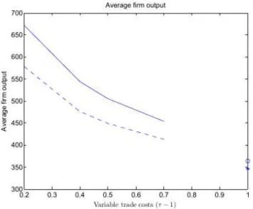
The second graphic shows that, when trade costs are smaller, only more productive firms stay in the market, competition is tougher, and, as consequence, average produc-tivity grows. Again, this effect is higher in comparative advantage industry. The third graphic present what happens with average firm output. We can see that, even with higher trade costs, average firm output is higher in commerce and it gets higher when trade costs fall. We also can view that comparative advantage firm always produce more, which is explained by the advantage comparative itself and because the average produc-tivity in this industry is also higher, as we have seen in the last graphic.

In the next graphic, ϕ_gDx/ϕg∗_Dx > ϕgDy/ϕg∗_Dy is always true. This happens because

Domestic country has comparative advantage in industry x. The graphic also shows that this difference becomes higher when trade costs fall, which means that liberalization magnifies comparative advantages in this economy, just as Bernard et al. (2007). The exporting probability rises when trade costs fall. Firms in comparative advantage industry have higher probability to export than firms in comparative disadvantage industry.

The next two graphics are about the mass of domestic firms and the mass of entrant firms respectively. The mass of firms producing domestically falls when the economy is opened, ZPC rises and less firms are able to continue producing. However, the mass of firms in comparative advantage industry is higher than in disadvantage industry. Al-though ZPC is higher in comparative advantage industry, when we open the economy, the probability of exporting is also higher in this industry. Hence, the expected profit ex-ante in this industry rises more than in comparative disadvantage industry and as con-sequence, the pool in this industry rises, while in the comparative disadvantage industry, it falls. Thus,the mass of domestic firms is higher in the comparative advantage indus-try. Analogously, in comparative advantage industry, when trade costs fall, the mass of entrants firms rises, and in comparative disadvantage industry falls.

Figure 1: Zero-profit and export cut-offs

Figure 3: Average firm output

Figure 5: Exporting probability

Figure 7: Mass of entrants

that, when trade costs are lower, indirect utility is higher. We obtain trade gains as Melitz (2003), most productive firms export and demand more labour, then, wages get higher, and, as consequence, less productive firms stop to produce. We also have trade gains like in Melitz and Ottaviano (2008), mark-ups are free to vary, then when the economy moves from autarky to an open economy, competition rise, then, firms set low mark-ups, thus, less productive firms stop to produce. Furthermore, trade gains are magnified in comparative advantage industry, just like in Bernard et al. (2007). Our model allow trade gains that all these previous models permit, but at one unique framework.

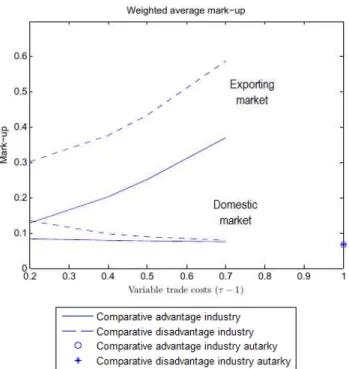
Average mark-up is always constant, in intention to analyse the effect of variable mark-ups, we calculate a weighted average mark-up. It is weighted by the proportion of output of each firm.

\ µ(ϕrh) =

Z ∞

ϕrh

µ(ϕ, ϕDh) yrh(ϕ)

Yrh dϕ.

Where, Yrh is the total output of industry h at market r.

Yrh = Nrh

Z ∞

ϕrh

yrh.g(ϕ|ϕ > ϕrh)dϕ

= NrhγhIhϕrh

wβh s w1

−βh u

η1

Where η1 = k

R∞

1 (W(xe)−1)/(W(xe)x

k_{)dx is constant depending on parameter k.}

Calculating µ\(ϕrh);

\ µ(ϕrh) =

η2 Nrhη1

.

Where η2 =k

R∞

1 (W(xe)−1)

2_/(W(xe)xk_)dx.

Figure 9: Weighted average mark-ups

We constructed this weighted average mark-up with the proposal to analyse the effects described previously, and to show a result that there isn’t present neither in Bernard et al. (2007) or Melitz and Ottaviano (2008).

6

Conclusion

Our main objective in this paper was to formulate a model that was capable to jointly provide trade gains via two different channels. On one hand, liberalization should shift up labour demand, thus, those firms there were less productive wouldn’t be able to produce after liberalization and would stop to produce. On the other hand, liberalization should make competition “tougher”, thus, mark-ups would get lower and firms that were less productive would stop to produce.

We developed a model of comparative advantage that incorporates heterogeneous firms and endogenous mark-ups that respond to the toughness of competition in a market. In such environment, we accomplished our main objective. We presented several results from Bernard et al. (2007) and from Melitz and Ottaviano (2008).

Market size influences firms in a specific industry: larger market size exhibits firms with larger profits and larger producing cutoff. Tougher competition result in lower mark-ups. However, average mark-up is constant. This is a weakness of our specification. As in Melitz and Ottaviano (2008), it would be better if tougher competition result in lower average mark-ups. Because of this, our model has a constant measure Nh of available

goods in each sector, this means that when trade costs fall, the economy present import substitution, although, consumers utility has “love of variety”.

Endogenous mark-ups permit mark-ups to vary when the economy moves form au-tarky to an opened economy and they influence each firm individually, they affect profits, and, as a consequence, if the firm will keep producing or not. However average mark-up do not change, so endogenous mark-ups does not present any results in the industry level. Thus, some results remain identical to those found by Bernard et al. (2007). Trade results in gross job creation and gross job destruction in both industries, and the magnitude of these gross job flows varies across countries and industries with comparative advantage.

Taking account welfare gains, our model, as in Bernard et al. (2007), has distinct implications for the distribution of income across factors. In our model it is possible to the real wage of scarce factor also rises with trade liberalization, or, at least, declines less than in Neoclassical models and in the predicted by the Stolper-Samuelson Theorem.

Differently form Bernard et al. (2007), our framework permit us to determinate closed solutions for all endogenous variables.

We also made a numeric exercise, where we showed many of the theoretical results and how endogenous variables change when trade costs fall. In this numerical exercise we constructed a weighted average mark-ups, thus, it do vary when the economy moves from autarky to an open economy. The result is that when the market has a tougher environment, the weighted average mark-up is smaller.

Although the model present constant average mark-up, our framework don’t present constant mark-ups. It is closer to the reality than assuming constant mark-ups for all firms. Hence, using our model, empirical studies will still use an constant average mark-up, but the model will comport the data, that will have different mark-ups. We believe that it could be an important contribution.

We used indirect utility to evaluate welfare gains. However, other papers used the compensating variation associated with a change in trade costs ((Arkolakis et al., 2012), Arkolakis, Costinot, Donaldson, and Rodr´ıguez-Clare (2012), Arkolakis et al. (2010)), Arkolakis, Costinot, Donaldson, and Rodr´ıguez-Clare (2012) have as result that welfare gains are lower when mark-ups are allowed to vary because there is incomplete pass-through of changes in marginal costs from firms to consumers, this means that firms tend to raise their mark-ups.

References

Arkolakis, C., A. Costinot, D. Donaldson, and A. Rodr´ıguez-Clare (2012). The elusive pro-competitive effects of trade. Working Paper.

Arkolakis, C., A. Costinot, and A. Rodr´ıguez-Clare (2010). Gains from trade under monopolistic competition: A simple example with translog expenditure functions and pareto distributions of firm-level productivity. mimeo.

Arkolakis, C., A. Costinot, and A. Rodriguez-Clare (2012, February). New Trade Models, Same Old Gains? American Economic Review 102(1), 94–130.

Asplund, M. and V. Nocke (2006). Firm Turnover in Imperfectly Competitive Markets -super-1. Review of Economic Studies 73(2), 295–327.

Aw, B. Y., S. Chung, and M. J. Roberts (2000, January). Productivity and Turnover in the Export Market: Micro-level Evidence from the Republic of Korea and Taiwan (China). World Bank Economic Review 14(1), 65–90.

Bernard, A. B. and J. Bradford Jensen (1999, February). Exceptional exporter perfor-mance: cause, effect, or both? Journal of International Economics 47(1), 1–25. Bernard, A. B., J. Eaton, J. B. Jensen, and S. Kortum (2003, September). Plants and

Productivity in International Trade. American Economic Review 93(4), 1268–1290. Bernard, A. B., J. B. Jensen, and P. K. Schott (2006, July). Trade costs, firms and

productivity. Journal of Monetary Economics 53(5), 917–937.

Bernard, A. B., S. J. Redding, and P. K. Schott (2007). Comparative Advantage and Heterogeneous Firms. Review of Economic Studies 74(1), 31–66.

Bowen, H. P., E. E. Leamer, and L. Sveikauskas (1987, December). Multicountry, Mul-tifactor Tests of the Factor Abundance Theory. American Economic Review 77(5), 791–809.

Clerides, S. K., S. Lach, and J. R. Tybout (1998, August). Is Learning By Exporting Important? Micro-Dynamic Evidence From Colombia, Mexico, And Morocco. The Quarterly Journal of Economics 113(3), 903–947.

Davis, D. R. and D. E. Weinstein (2001, December). An Account of Global Factor Trade. American Economic Review 91(5), 1423–1453.

Feenstra, R. C. (2003, January). A homothetic utility function for monopolistic compe-tition models, without constant price elasticity. Economics Letters 78(1), 79–86. Helpman, E. (1984, 00). Increasing returns, imperfect markets, and trade theory. In

R. W. Jones and P. B. Kenen (Eds.),Handbook of International Economics, Volume 1 of Handbook of International Economics, Chapter 7, pp. 325–365. Elsevier.

Helpman, E., M. J. Melitz, and S. R. Yeaple (2004, March). Export Versus FDI with Heterogeneous Firms. American Economic Review 94(1), 300–316.

Krugman, P. R. (1981, October). Intraindustry Specialization and the Gains from Trade. Journal of Political Economy 89(5), 959–73.

Markusen, J. R. and A. J. Venables (2000, December). The theory of endowment, intra-industry and multi-national trade.Journal of International Economics 52(2), 209–234. Melitz, M. J. (2003, November). The Impact of Trade on Intra-Industry Reallocations

and Aggregate Industry Productivity. Econometrica 71(6), 1695–1725.

Melitz, M. J. and G. I. P. Ottaviano (2008). Market Size, Trade, and Productivity. Review of Economic Studies 75(1), 295–316.

Pavcnik, N. (2002). Trade Liberalization, Exit, and Productivity Improvements: Evidence from Chilean Plants. Review of Economic Studies 69(1), 245–276.

Rodr´ıguez-L´opez, J. A. (2011). Prices and Exchange Rates: A Theory of Disconnect. Review of Economic Studies 78(3), 1135–1177.

Scheve, K. and M. J. Slaughter (2004). Economic insecurity and the globalization of production. American Economic Journal of Political Science 93, 686–708.

Schott, P. K. (2003, June). One Size Fits All? Heckscher-Ohlin Specialization in Global Production. American Economic Review 93(3), 686–708.

Schott, P. K. (2004, May). Across-product Versus Within-product Specialization in In-ternational Trade. The Quarterly Journal of Economics 119(2), 646–677.

Trefler, D. (1993, December). International Factor Price Differences: Leontief Was Right! Journal of Political Economy 101(6), 961–87.

Trefler, D. (1995, December). The Case of the Missing Trade and Other Mysteries. American Economic Review 85(5), 1029–46.

Yeaple, S. R. (2005, January). A simple model of firm heterogeneity, international trade, and wages. Journal of International Economics 65(1), 1–20.

7

Appendix

Proposition 2.1. The mass of available goods in each industry depends only on the substitutability among varieties;

Nh =

1

γh(ln ˆph−lngph)

= 1

γhµe(k)

. (27)

Proof. First, we need to findlnpfh. Using the equation forph(ϕ) and the following property

of lambert function W, that ln|W(x)|=lnx− W(x)∀x >0, we have that,

lnph =ln

(ws)βh(wu)1−βh ϕh

−µh(ϕ).

Then, we have that,

f

lnph =ln

(ws)βh(wu)1−βh ϕh

−_eµ(k) = lnp_bh−eµ(k).

Rearranging this we have that lnp_bh−lnpfh =µe(k). From definition ofpbh we have that

Nh =

1

γh(ln ˆph −lngph) .

Substituting lnp_bh−lnpfh =µe(k) we have the result. Nh is constant and equal for both

countries.

Proposition 2.2. Expenditures on entry investment employment are equal to profits in each sector.

NEhfE(ws)βh(wu)1

−βh _{= Π} h.

Proof. Total profit of industry h, Πh is

Πh =Nh

Z ∞

ϕh

πh(ϕ)g(ϕ|ϕ ≥ϕh)dϕ=NhγhIhχe(k).

Using FEC, we have that:

NEhfE(ws)βh(wu)1

−βh _=N ph

ψhIh ϕk

h

=Nph

_ϕ

ϕh

k

γhIhχe(k) = Πh.

proposition2.3.Equilibrium wages defined only on comparative advantage parame-ters.

wu ws

= 1−(αβx+ (1−α)βy) (αβx+ (1−α)βy)

Proof. Using Labour market clearing conditions, we have that Lkh = LDpkh +LEkh.

Us-ing Shepard’s Lemma and cost functions, we can calculate enterUs-ing labour demand and producing labour demand, for k=s:

LE

sh =NEhfEβh(wu/ws)1

−βh_.

And,

LDp_sh(ϕ) = βh(wu/ws)

(1−βh)

ϕ yh(ϕ).

Then,

LDp_sh = Nh

Z ∞

ϕh

LDp_sh(ϕ)g(ϕ|ϕ > ϕh)dϕ

= Nh

βhγhIh ws

e

φ(k)

Where φe(k) = kR₁∞WW(xe)_(xe)−1

1

xk+1dx. Then, Lsh =δNphfEβh(wu/ws)1

−βh_+N h

βhγhIh ws

e

φ(k).

Using the definition of Nph and the cutoff ϕh, we have that;

Nph=Nh

ϕh ϕ

k

=Nh

γhχe(k)Ih δfEwsβhw1

−βh u

.

Thus, substituting it and Nh in the last equation, we have that,

Lsh =

βhIh wseµ(k)

(χ_e(k) +φe(k)).

We know that, χ_e(k) +φe(k) = µ_e(k) and wsLs=ws(Lsx+Lsy), thus;

wsLs = βxαI +βy(1−α)I

= (αβx+ (1−α)βy)(wsLs+wuLu)

Rearranging;

wu ws

= 1−(αβx+ (1−α)βy) (αβx+ (1−α)βy)

Ls Lu .

Claim 3.1. There is no opportunity of arbitrage in the economy.

1. pXh(ϕ)/τh < pDh(ϕ). There is no profitable export resale by a third party of a good

produced and sold in a country.

2. pDh(ϕ)/τh < pXh(ϕ). There is no profitable resale of a good exported to a country,

Proof. 1. We have that ∂µrh(ϕ, ϕrh)/∂ϕrh < 0, thus, µXh(ϕ) < µDh(ϕ)). Then we

have that:

pXh(ϕ) τh

= (1 +µXh(ϕ))

(ws)βh(wu)1−βh

ϕ <(1 +µDh(ϕ))

(ws)βh(wu)1−βh

ϕ =pDh(ϕ).

2.

pXh(ϕ) = W

ϕ ϕXh e τh

(ws)βh(wu)1−βh ϕ = W ϕ ϕ∗ Dh ϕ∗ Dh ϕXh e ϕXh ϕ∗ Dh

(w∗

s)βh(w

∗

u)1

−βh

ϕ

= p∗

Dh ϕϕ ∗ Dh ϕXh

In the second equality we use equation (17), now we will use what we already proved in item one and repeat this procedure to find our result.

p∗ Dh ϕϕ ∗ Dh ϕXh

> p∗

Xh ϕϕ ∗ Dh ϕXh 1 τh

=pDh

ϕϕ ∗ Dh ϕXh ϕDh ϕ∗ Xh 1 τh

=pDh

ϕ τ2 h 1 τh

> pDh(ϕ)

1

τh .

In the second equality we used equations (18) and (19). Note that now we have

pDh(ϕ)/τh < pXh(ϕ).

Proposition 3.2. The average prices andln average prices of domestic and imported goods are equal.

e

ph =peDh=pe

∗

Xh e pe

∗

h =pe

∗

Dh =epXh,

f

lnph =lnpfDh =lnpf

∗

Xh e lnpf

∗

h =lnpf

∗

Dh =lnpfXh.

Proof. First, let’s find p_eDh. We can write pDh(ϕ) as

pDh(ϕ) =W

ϕ ϕDh

e

(ws)βh(wu)1−βh

ϕ .

Then, p_eDh is given by,

e

pDh =

Z ∞

ϕDr W

ϕ ϕDh

e

(ws)βh(wu)1−βh ϕ

kϕk Dh

ϕk+1dϕ.

Applying change of variables, x=ϕ/ϕDh, we have that,

e

pDh =v(k)

(ws)βh(wu)1−βh

ϕDh

.

Where, v(k) =kR₁∞W(xe)/xk+2_{dx is a constant function of the parameter k.}

e

p∗

Xh=v(k)τh

(w∗

s)βh(w

∗

u)1

−βh

ϕ∗

Xh .

From equation (16), we have that, (ws)βh(wu)1−βh

ϕDh

=τh

(w∗

s)βh(w

∗

u)1

−βh

ϕ∗

Xh .

Thus, p_eDh=pe∗Xh=peh. Repeating this argument, we have that pe∗Dh =peXh =pe∗h.

For the second part, we start by findinglnpfDh. Using the equation forpDh(ϕ) that was

used before and the property of lambert functionW, thatln|W(x)|=lnx− W(x)∀x >0, we have that,

lnpDh=ln

(ws)βh(wu)1−βh

ϕDh

−µDh(ϕ).

Integrating both sides between ϕh amd ∞.

f

lnpDh =ln

(ws)βh(wu)1−βh

ϕDh

−µ_e(k).

Analogously, for the prices of imported goods

f

lnp∗xh =ln

τh

(w∗

s)βh(w

∗

u)1

−βh

ϕ∗

Xh

−_eµ(k).

From relation (16), and we have that (ws)βh(wu)1−βh

ϕDh =τh

(w∗

s)βh(w∗u)1−βh ϕ∗

Xh . Then,

f

lnp_Dh =

f

lnp∗_xh =lnpf_h. Again, we can repeat this process and show that, lnpf_Dh∗ =lnpf_xh =lnpf∗_h.

Proposition 3.3. The mass of available goods in each industry depends only on the substitutability among varieties;

Nh =

1

γh(ln ˆph−lngph)

= 1

γheµ(k)

=N∗

h. (28)

Proof. From 3.2 we know that,

f

lnph =ln

(ws)βh(wu)1−βh

ϕDh

−_eµ(k) = lnp_bh−eµ(k).

Rearranging this we have that lnp_bh−lnpfh =µe(k). From definition ofpbh we have that

Nh =

1

γh(ln ˆph −lngph) .

Substituting lnp_bh−lnpfh =µe(k) we have the result. Nh is constant and equal for both

countries.

Proposition 3.4. Expenditures on entry investment employment are equal to profits in each sector.

NEhfE(ws)βh(wu)1