Education, preferences for leisure, and the optimal income tax schedule

Fundação Getulio Vargas

Escola de Pós-Graduação em Economia

FGV-EPGE

EDUCATION, PREFERENCES FOR LEISURE, AND THE

OPTIMAL INCOME TAX SCHEDULE

Tiago Pedroso Severo

Fundação Getulio Vargas

Escola de Pós-Graduação em Economia

FGV-EPGE

EDUCATION, PREFERENCES FOR LEISURE, AND THE

OPTIMAL INCOME TAX SCHEDULE

Dissertação a ser submetida à Escola de Pós-Graduação em Economia da Fundação Getulio Vargas como requisito para obtenção do Título de Mestre em Economia.

Aluno: Tiago Pedroso Severo

Orientador: Carlos Eugênio Ellery Lustosa da Costa

Ficha catalográfica elaborada pela Biblioteca Mario Henrique Simonsen/ FGV

Severo, Tiago Pedroso

Education, preferences for leisure, and the optimal income

Tax schedule / Tiago Pedroso Severo. – 2006. 32 f.

Orientador: Carlos Eugênio Ellery Lustosa da Costa. I nclui bibliografia.

1. I mposto de renda. 2. Educação e Estado. I . Costa, Carlos Eugênio da. I I . Fundação Getulio Vargas. Escola de Pós- Graduação em Economia. I I I . Título.

FUNDAÇÃO

GETULIO VARGAS

EPGE

Escola de Pós-Graduação em Economia

LAUDO SOBRE DISSERTAÇÃO DE MESTRADO

TERMO DE APROVAÇÃO

TIAGO PEDROSO SEVERO

EDUCATION, PREFERENCES FOR LEISURE, AND THE OPTIMAL INCOME TAXSCHEDULE

Tese aprovada como requisito parcial para obtenção do grau de Mestre em Economia no Programa de

Mestrado em Economia desta Escola de Pós-Graduação em Economia da Fundação Getulio Vargas. O

aluno tem um prazo máximo de 3 meses para envio da versão final da Dissertação de Mestrado.

Banca Examinadora:

Prof. Carlos Eugêni Ellery Lustosa da Costa (Orientador)

EPGE/FGV

I

X/

Prof. Luis Henrique B. Braido

E GE/FGV

. I

ｦｾｍｳｦＬ ｵｮ￧￣ｯ＠

Rio de Janeiro, I O de maio de 2006

Education, Preferences for Leisure and the Optimal Income

Tax Schedule.

Tiago Severo†

Getulio Vargas Foundation

Abstract

Recent advances in dynamic Mirrlees economies have incorporated the treatment of human capital investments as an important dimension of government policy. This paper adds to this literature by considering a two period economy where agents are differentiated by their preferences for leisure and their productivity, both private in-formation. The fact that productivity is only learnt later in an agent’s life introduces uncertainty to agent’s savings and human capital choices and makes optimal the use of multi-period tie-ins in the mechanism that characterizes the government policy. We show that optimal policies are often interim inefficient and that the introduc-tion of these inefficiencies may take the form of marginal tax rates on labor income of varying sign and educational policies that include the discouragement of human capital acquisition. With regards to implementation, state-dependent linear taxes implement optimal savings, while human capital policies may require labor income taxes that depend directly on agents’ schooling. Keywords: Income Taxation; Educational Policy; Dynamic Screening. JEL Classification: H21; D63

1

Introduction

Two important shortcomings of Mirrlees’ (1971) framework are its static nature and its relying on overly restrictive assumptions on the degree of heterogeneity between agents. Not surprisingly, the most important and challenging modifications are exactly the introduction of dynamic concerns and other dimensions of heterogeneity among agents. Despite the effort, the technical difficulties are well known,1 _{and advances in}

the area, slow.

∗_{We thank Juliano Assun¸c˜ao, Luis Braido, Cristiano Costa, Lucas Maestri, Paulo Monteiro, Claudia}

Rodrigues, participants at the SBE meeting and seminar participants at EPGE and PUC-Rio for their comments. All errors are ours.

†_{E-mail: tsevero@fas.harvard.edu} 1

This paper adds to our knowledge of non-linear optimal income taxation in a multi-dimensional dynamic setting and, at the same time, incorporates another important dimension of government actions: human capital policies. Human capital investments have been shown to have important quantitative consequences for the design of labor income taxes [e.g., Kapicka (2006)], while human capital policies have been shown to depend on the richness of government policy instruments [e.g., da Costa and Maestri (2007)].2 We revisit both issues and characterize policies along the whole (constrained) Pareto frontier.

Multidimensionality in our model is due to the fact that agents differ both with re-spect to their preferences for leisure and their productivity. Both are private information. Uncertainty arises from the fact that agents only learn their productivities later in life, after some life-long choices have been made. We follow, in this sense, the new dynamic public finance literature in considering a setting where information is private but only gradually learnt by the agents.

Early in life, when human capital investments are made, agents are separated in two preference types, the lazy agents and the hard workers, distinguished by their disutility of effort, be it in forming human capital, or be it in supplying labor to the market. The return to investment in human capital is uncertain since agents only learn their raw productivity, which will be composed with human capital to determine earnings capacity, later in life. After uncertainty is realized, agents choose how much labor to supply in the market, their after tax earnings being used to pay for life-time consumption.

A benevolent government which inhabits this economy, and is restricted by its in-formational structure solves a Pareto problem that we show to be associated with a particular cost minimization program, that possesses nice separable structure. We take advantage of this separability to investigate the optimal allocations for each preference class of agents separately, and to highlight the influence of insurance and redistributive motives in determining the sign of all wedges created by the government.

For all (constrained) Pareto efficient allocations it is possible to show that lazy agents never face negative marginal income taxes, and the most productive hard worker agent never faces positive marginal income taxes. The marginal tax rate for the least productive hard working agent may, however, take any sign. Similarly one can no longer guarantee that the encouragement of human capital derived in da Costa and Maestri (2007) remains optimal in our context. Our problem lacks what Fernandes and Phelan (2000) have termed common knowledge of preferences since, in the second period, agents’ preferences

2

depend on the type she realized when she was born, which is private information. For this very same reason, policies will be characterized by an element of interim inefficiency since, once first period choices are made, and preference types revealed, all agents would profit from redefining their budget sets.

It is in this context that marginal tax rates on labor income must be understood. If the government were allowed to re-optimize after agents revealed their preference types and possibly made their consumption and human capital choices, the second budget sets of both types of agents would be the one derived from solving a Mirrlees program. The solution to this insurance problem is well known: the high productivity agents faces a zero marginal tax rate and the low productivity agent faces a strictly positive marginal tax rate. The problem is that, when the government faces an agent who claims to be say a low productivity hard worker, it must take into account not only that the agent is lying about her productivity, but also that she has lied in the past about her preferences. To preclude false announcements in the first period, distortions are created in the second period allocations that cease to be useful once preference types are revealed. Implicit in our model is a commitment technology through which the government commits not to change the budget sets even if it is in everyone’s interest to do so.

The lack of common knowledge of preferences will also affect human capital policies. In a world with ex-ante identical agents, da Costa and Maestri (2007) have shown that

it is always optimal to encourage human capital formation.3 _{The rationale for their}

result is as follows. If agents are ex-ante identical, the government intervention has the sole purpose of providing insurance from raw productivity shocks. Because these shocks are private information, redistributive policies are restricted by this informational asymmetry. In particular, at the optimum, the government has to guarantee that an agent who receives a high productivity shock does not try to get the transfers to which an agent who received a bad shock is entitled, by shirking and reducing labor supply. When human capital choices are made, an agent does not know her productivity but anticipates the choices that she will make in any state of the world. If she intends to get the transfer, even if she realizes the high productivity shock, she anticipates lower labor supply and under-invest in human capital. Encouraging human capital formation increases the cost of reducing labor supply thus making less attractive this deviating strategy.

In our model the encouragement of human capital choices need no longer be optimal. First the distortions created in second period allocations may be such that the govern-ment is worried about agents supplying more, rather than less, labor than the optimal. This being the case, agents who anticipate this type of deviation will over-invest, instead

3

of under-invest, in human capital. Second, even if agents within the same preference class under-invest in human capital when they intend to deviate, the agents that choose the budget set for the agents of a different preference class may over-invest in human cap-ital, theoretically making the discouragement of human capital formation an important instrument for precluding false announcement of preferences. Despite this, we show that, whenever differences in productivity are more important than differences in preferences, in a sense to be made precise later, it will be optimal to (weakly) encourage human capital formation for the two types of agents and at all points of the Pareto frontier.

We also produce some numerical examples to illustrate the situations theoretically described and to calculate, for each situation, the associated labor income taxes and human capital distortions. In our numerical exercises, the discouragement of human capital is never optimal.

As for implementation Kocherlakota (2004, 2005a), Albanesi and Sleet (2006) have shown that optimal taxes on savings must be dependent on second period information. The same is true here. As for education, in our model, its costs is disutility of effort, which makes direct taxation somewhat artificial. However, student loans which are often used by governments can help induce individuals to spend some extra time at school if interest rates differ from those of regular loans. The implicit tax structure on education becomes formally equivalent to that on savings. We show, however that this instrument induces optimal choices if the allocation is interim Pareto efficient, but does not suffice when interim inefficiencies are present, in which case, some income taxes that depend directly on the educational level of agents to implement the optimum will be needed.

The inter-temporal nature of the problem as well as the existence of two dimensions of unobserved heterogeneity makes the problem too hard to handle in its full generality. Some crucial simplifying assumptions are made to keep the problem tractable while at the same time maintaining the richness of the environment. First, we assume that preferences are such that marginal rates of substitution are exogenously ordered, which avoids our having to handle endogenously determined chains of incentive compatibility constraints. Second, we assume that the conditional distribution of productivity shocks are independent of an agent’s type. This rules out an extra source of informational advantage of agents off the equilibrium path. Finally, our relying on only two types of agents and only two different productivity levels allows us to derive very sharp results along some dimensions of policy, which we believe would not be possible in more complex environments. We view this simplicity as one of the strengths of our paper in that it allows us to clearly identify the forces that are hard to separate in more general frameworks.

cost minimization problem that we shall explore. In section 3 we present the general separable problem and solve for a particular case that will prove a useful benchmark. We investigate the optimal allocations for lazy agents in section 4 and for hard workers in section 5. In section 6, we describe one of the possible tax systems that implement optimal allocations and show that linear taxes on human capital will not suffice. Section 7 presents an example that shows that power to make agents commit to a certain budget set before they know their productivities allows the government to attain Pareto superior allocations, even if no other choices are made early in life. Section 8 concludes. Proofs are collected in the appendix.

2

The Economy

Ours is a small open economy populated by a continuum of individuals of two

dif-ferent types, hard workers and lazy agents, in proportions π and π of the population,

respectively.

Agents live for two periods, youth and adulthood and have preferences over de-terministic sequences of effort, e ∈ [0,e¯], and consumption, c ∈ R+, represented by

P

t=0,1

u(ct)−αeδt/δ ,withδ >1.Functionu(·) is strictly increasing and concave and

satisfies Inada conditions, limc→0u′(c) = ∞ and limc→∞u′(c) = 0. The difference

be-tween hard workers and lazy agents is the parameter α:α for the former and α for the latter, with α > α >0.

The production technology isy =whl: output, y, is produced from labor efficiency units, whl, wherel is working time,h is human capital andw is raw productivity, with a fixed coefficient technology which we normalize to one is transformed in the single

consumption good at a fixed rate of one. Human capital is produced from effort with

one period lag, which means that human capital formed in the second period is useless. All second period effort is, therefore, labor supply. For simplicity, we assume that effort in the first period can only be used for human capital formation.

Uncertainty in this model arises because agents only learn their raw productivity,w, in the second period of their lives. As we have done with preferences, we assume that

w can only take two values, wL and wH (wH > wL > 0), with probabilities πL and

πH, respectively, which we assume to be identical across preference types. Shocks are

independent and identically distributed across agents, which allows us to invoke the law of large numbers and rule out any form of aggregate uncertainty.

productivity is realized. Labor supply is chosen, and after tax earnings used to finance consumption in the second period and pay for first period consumption. Agents’ life-time expected utility is, therefore,

u(c1)−

α δh

δ₊X

i=H,Lπi

"

u(ci)−

α δ

yi

hwi

δ#

. (1)

The economy is competitive: workers and firms take wages and prices as given. Al-though firms cannot observew, they observe the level of output generated by each agent,

y. The zero-profit condition, along with the linearity of technology implies that, if there was no government intervention, the output produced by each agent is her labor income. I.e., absent government intervention, and assuming a zero exogenous interest rate, each

agent’s problem would be the maximization of (1) subject to c1 ≤ b and ci ≤ yi −b

(i=H, L), where bstands for borrowing andiis output produced if realized productiv-ity is wi. However, a benevolent government which inhabits this economy uses the tax

system to provide insurance for both types of agents and redistribute resources from one preference class to the other. In pursuing its goals the government is restricted by the

informational structure of the economy: both α and w are agents’ private information.

The government does observe (and has the instruments to control) the choices of c, h

and y.

As usual, we shall work directly with the allocations leaving the policy instruments in the background. In doing so, we adopt the following notation. We write first period consumption intended for a typeα agent asc(α).Human capital ash(α).In the second

period, however, w also differentiates agents and we write second period consumption

and supply of efficiency units intended for agent (α, i) as ci(α) and yi(α), i = H, L,

respectively.

[Insert Figure 1]

Let C ⊆ ℜ+ and Y ⊆ ℜ+ denote, respectively, the second period consumption

and effective labor spaces. The marginal rate of substitution between effective labor and consumption in the second period for an agent of type (α, i) at an allocation (y, c) in the Y ×C space is, for a given h, M RSi(α) ≡ αyδ−1(wih)−δu′(c)−1. It is not

hard to see that, at the same allocation, M RSi(α) ≶ M RSj(ˆα) ⇔ α/wiδ ≶ α/wˆ δj.

Therefore, at a given point in the Y ×C space, M RSH(α) < M RSL(α) < M RSL(α)

and M RSH(α) < M RSH(α) < M RSL(α). As for the ordering for M RSL(α) and

M RSH(α), it will depend on whether differences in preferences are more important

Definition 1 We say that differences in productivity are more important than differ-ences in preferdiffer-ences for leisure if

α wδ H

< α wδ

L

.

Otherwise, we say that differences in preferences for leisure are more important than differences in productivity.

The Pareto Problem An allocation for this economy is a pair (z(α), z(α)) where

z(α) ≡ nc(α), h(α),(ci(α), yi(α))i=L,H

o

for α = α, α. In words, an agent who an-nounces to be of typeα in the first period getsz(α) comprised of human capital invest-ment, h(α), that she must make and consumption,c(α), to which she is entitled, in the first period, and budget set, (ci(α), yi(α))i=L,H, from which she will choose in the second

period.

To define an incentive compatible allocation let us start with the second period choices. For concreteness consider the optimal strategy of a ˆα agent who announced to be of type α and define

ˆ

σi(α)∈arg max j

(

u(cj(α))−αˆ

δ

yj(α)

wih(α)

δ)

∀i, (2)

as (one of) her optimal announcement(s) of productivity if she realizes productivitywi.

The expected utility she attains by following her optimal announcement strategy is

U(z(α)|αˆ)≡u(c(α))−αˆ

δh(α)

δ₊X

iπi

"

u(c_σˆi(α)(α))−

ˆ

α δ

_y

ˆ

σi(α)(α) wih(α)

δ#

.

We shall be using the notation σi(α) and U(z(α)|α) for lazy and σi(α), U(z(α)|α)

for hard workers.

For an allocation to be incentive compatible it must be such that an agent who chooses the budget set intended for her (i.e., announces her preferences truthfully) finds it in her best interest to announce truthfully her productivity shock, i.e.,

σ_i(α) =iand σi(α) =ifor i=H, L. (3)

It must also guarantee that the agent chooses the budget set intended for her no matter what she does in the second period, i.e.,

Before moving on, a cautionary note is due. Incentive compatibility with regards to preference announcement, requires the agents to find it better to announce truthfully in the first period — and in the second, as guaranteed by (3) — than to announce falsely in the first period, regardless of what she does in the second which is guaranteed by (4). Notice, however that whenever the solution to (2) is not unique for an agent who announced falsely in the first period, all strategies that solve (2) must be included in the derivation of optimal allocations.

Strong separability between consumption and effort implies that at any efficient al-location there can be no idle resources in the economy. Were it not the case and con-sumption could be given to each type of agent in the first period of their lives in such a way to preserve differences in utility in this period. No incentive constraints would be violated and agents would be better off. Therefore, we may define efficient allocations as follows. An allocation is (constrained) Pareto efficient only if it minimizes

πnc(α) +X

iπi[ci(α)−yi(α)]

o

+πnc(α) +X

iπi[ci(α)−yi(α)]

o

(5) subject to

U(z(α)|α) =U , U(z(α)|α)≥U , (6)

(3) and (4).

We refer to constraints (6), as the promise-keeping constraints. The problem above defines a cost function E U , U

which level curves are associated with the utility pos-sibility frontiers for this economy.4 _{For each vector of relevant parameters and function}

u(·), the domain of E(·,·) is the set of pairs U , U

such that there are allocations

z(α) and z(α) that satisfy all the incentive compatibility constraints and such that

U(z(α)|α) = U and U(z(α)|α) = U. The set is not empty since the pair (UA,UA) corresponding to the utility attained by the autarchy allocation, trivially satisfies all the relevant constraints.

We shall, however, work with a different cost minimization problem in which con-straints U(z(α)|α) ≤U and U(z(α)|α) ≤U substitute for U(z(α)|α) ≥U(z(α)|α) and U(z(α)|α)≥U(z(α)|α). It is straightforward to see that if the cost minimization problem is solved this new problem must also be solved. The main advantage of this new problem is that it has a nice separable structure: the objective function is additive inz(α) and each constraint involves only the allocation associated to a single preference type. This allows us to find the allocation for each agent separately, taking the utility of the other agent as a parameter of the minimization problem, a procedure which not only facilitates the derivation of our results (and simplifies the problem in more complex

4

The level curvesdefinethe utility possibility frontiers if the solution to the minimization problem as well as the solution for the associated problem in which constraintsU(z(α)|α) =U , U(z(α)|α)≥U are replaced byU(z(α)|α)≥U , U(z(α)|α) =U is unique for all pairs U , U

environments) but also makes explicit the often conflicting goals of providing insurance to both agents and redistributing resources across agents. The redistributive aspects

being associated with the specific choices of U and U . Notice, however, that solving

the latter problem for an arbitrary pair (U , U) in the domain of the problem does not imply that a particular Pareto problem is solved. Even though the solution to this latter problem gives us the minimum cost of delivering utilities U and U, it does not rule out the existence of another pair (U′_{, U}′_{) such that U}′ _{≥ U and U}′ _{≥ U , with one of the}

inequalities strict such that the pair (U′_{, U}′_{) can be delivered at a weakly lower cost.}

Increasing the utility of an agent, on the one hand, requires more resources, which tends to force a reduction of the utility of the other agent, while on the other, relaxes incentive compatibility constraints which may allow for an increase in the agent’s utility.5 Yet, because agent α’s allocation only appears in the incentive compatibility constraint of agentα’s problem through its effect on the equilibrium utility of agent α,the first order conditions with respect to z(α) and z(α) of the Pareto problem and the problem we examine are identical up to a redefinition of Lagrange multipliers. We may, therefore, characterize all distortions on agents’ choices using either problem. This highlights an important aspect of optimal allocations: their distortions depend not on the behavior of the agent to whom the contract is intended but on the behavior of those who may envy it.

2.1 Discussion

From a second period perspective, agents are characterized by two exogenous param-eters, α, a preference parameter that represents costs associated with work (or human capital investment) while the second,w, is a productivity parameter. As is well known,

we may associate to each type (α, i) an index thus reducing the problem to a single

dimensional screening problem. The trouble with this procedure, in general, is that, in collapsing the tow dimensions in a single one, single-crossing is usually lost, chains of relevant incentive constraints become endogenous and the complexity of the problem

substantially increased.6 _{We have chosen a functional form for preferences that}

pre-serves an exogenous ordering of marginal rates of substitution, greatly simplifying the characterization of optimal allocations.

Preferences defined in (1) have another interesting property related to the first order

condition for human capital choices, h2δ = P

iπi(yi/wi)δ which differ for agents of

different preferences only insofar as their labor supply choices differ. As we shall see, this property will be very useful in determining the direction of human capital policies.

5

We thank an anonymous referee for pointing that out. For a similar discussion, see Brito et al. (1990).

6

Another important assumption we adopt is the independence of πi on an agent’s

preferences. If the probability of realizing a given probability shock depended on an agent’s preferences, this would create what Fernandes and Phelan (2000) termed ‘lack of common knowledge of preferences’, in which case, an agent’s history of choices would not be a sufficient statistic for her preferences over future actions.7 _{Our assumption}

on the distribution of shocks rule this out. We do so to concentrate in another source of lack of common knowledge. To use the language of Fernandes and Phelan, we may think of agents history beginning with a shock of preferences in the beginning of period 0. This privately observed history will influence an agent’s preferences over second pe-riod bundles, thus generating lack of common knowledge of preference. Second pepe-riod’s allocations will have to be chosen in such a way as to avoid gains for agent’s that de-viate in the announcement of their preferences. As in their case, an element of interim inefficiency will be introduced.

3

The Main Program

In characterizing optimal policies, of concern are wedges between marginal costs and benefits of agents’ choices induced by the government. These wedges reflect directions toward which private choices are distorted. Technology is characterized by a constant unitary marginal rate of transformation,M RT, between effective labor and consumption, therefore, absent government intervention, a competitive equilibrium is characterized by

M RSi(α) = M RT = 1 for all (α, i). Government policies introduce wedges between

the M RS and the M RT. We shall refer to such wedges—which may differ at different

allocations with non-linear tax schedules—as the ‘marginal’ income tax rate, θ(y) ≡

M RT −M RS = 1−M RS.8

Similarly, absent government policies, the first order condition for human capital choice, is h2δ = P

iπi(yi/wi)δ. If this equality holds at the constrained optimal

allo-cation, we say that human capital in not distorted. If however, h2δ _> P

iπi(yi/wi)δ,

we say that human capital formation is encouraged (weakly encouraged if the inequality is not strict). Finally, we say that human capital formation is discouraged when the opposite inequality holds at the optimum.

Bearing this in mind, we now explore the separability in the planner’s cost minimiza-tion problem and discuss one at a time the design of (constrained) optimal allocaminimiza-tions for each class of preferences, emphasizing the relevant wedges associated with each type’s

7

Some of the issues that arise in such context have been explored by Fernandes and Phelan (2000), themselves, and by Golosov and Tsyvinsky (2006), for example.

8

allocations.

To do so we first spell out the Lagrangian associated with the program that charac-terizesα-type agent’s (for α=α, α) allocations. We call itα-type program.

α-type Program:

minc(α) +X

iπi[ci(α)−yi(α)]

subject to

u(c(α))− α

δh(α)

δ₊X

iπi

"

u(ci(α))−

α δ

yi(α)

wih(α)

δ#

=U, (Φ)

u(ci(α))−

α δ

yi(α)

wih(α)

δ

≥u(cj(α))−

α δ

yj(α)

wih(α)

δ

i6=j, (λi)

and

ˆ

U ≥u(c(α))−αˆ

δh(α)

δ₊X

iπi

"

u(c_σˆi(α)(α))−

ˆ

α δ

_y

ˆ

σi(α)(α) wih(α)

δ#

. (Ψ)

The Lagrange multipliers associated with each constraint are displayed to the right of the equation. We shall, at times, abuse language and refer to the incentive con-straint through the Lagrange multiplier associated to it. Note also that all variables and functions with hats are associated with type ˆα agent, for ˆα=α,α.

Incentive compatibility requires ˆαtype not to find in her interest to announce falsely her preferences, independently of her announcement strategy in the second period. Con-straint (Ψ) guarantees just that. If the optimal announcement strategy is not unique, i.e., the set defined in (2) is not a singleton, Ψ is a vector with one entry associated with each off-equilibrium strategy in the set.

Notice also that when both second period constraints bind at the optimum, i.e.,

λH > 0, λL > 0, lazy agents are bunched. In Mirrlees setting, this is the only sense

in which bunching is defined. Here, however, we could, in principle, have another type of bunching, which we refer to as first period bunching, if the two preference types were assigned the same ‘contract’, i.e., z(α) = z(α). It is possible to show, however, that bunching the contracts is never optimal — lemma 3. Therefore, in what follows, whenever we refer to bunching it should read second period bunching: the assignment of a single bundle to agents of different productivities and the same preference type.

would anticipate these mutually agreed changes and would not announce truthfully. We assume that the government possesses a commitment technology that precludes it from re-optimizing. We shall at times refer to allocations in which Ψ binds as interim inefficient and those for which the constraint does not bind asinterim efficient.

We next characterize interim efficient allocations.

Proposition 1 If constraintΨ is slack inα-type program, then: i) the most productive α faces a marginal income tax rate of zero; ii) the least productive α faces a positive marginal income tax rate, and; iii) human capital formation by α is encouraged.

Interim efficient allocations represent an important benchmark for the policies we will be discussing. If the value of α-type program is zero, and the allocation is interim efficient we have a pure insurance policy. Notice however that deviations from interim efficiency need not represent a redistributive motive. The pure insurance program for agentαmay be preferred by agent type ˆαeven if ˆαis offered her pure insurance program, i.e., even if there is no redistribution between the agents. The reason why this may be the case is because, even though there is no redistribution in equilibrium, there may be off-equilibrium.

In what follows we concentrate on interim inefficient policies. We do this for the two different configurations of the economy. First, for the case in which differences in productivities are more important. Then, for the case in which difference in preferences for leisure are more important.

4

Lazy’s Allocations

Having already characterized interim efficient allocations for any type α, we shall now focus on interim inefficient allocations for lazy agents. The first step toward this end is to carefully investigate constraint(s) (Ψ).

Lemma 1 If differences in preferences for leisure are more important than differences in productivities, off-equilibrium hard workers always announce to be of high productivity. If, however, differences in productivities are more important, off-equilibrium hard workers always announce truthfully in the second period.

According to lemma 1: i)the set defined in (2) is a singleton; ii)when differences in preferences are more important, constraint (Ψ) in Lazy agent’s program reads

U ≥u(c(α))−α

δh(α)

δ_+u(c

H(α))−

α δ

X

iπi

yH(α)

wih(α)

δ

and; iii)when differences in productivities are more relevant, it reads

U ≥u(c(α))−α

δh(α)

δ₊X

iπi

"

u(ci(α))−

α δ

yi(α)

wih(α)

δ#

.

Marginal Income Taxes Taking into account lemma 1, whenever differences in pref-erences for leisure are more important, the first order conditions of the Lagrangian as-sociated with α-type program with respect tocH(α) and cL(α) are, respectively,

u′(cH(α)) =πH[ΦπH +λH −λL−Ψ]−1 and u′(cL(α)) =πL[ΦπL+λL−λH]−1.

First order conditions with respect to yH(α) and yL(α) are

αyH(α)δ−1

h(α)δ_wδ H

=πH

(

ΦπH +λH −λL

wH

wL

δ

−Ψα

α

X

iπi

wH

wi

δ)−1

.

and

αyL(α)δ−1

h(α)δ_wδ L

=πL

(

ΦπL+λL−λH

wL

wH

δ)−1

,

respectively.

It is possible to show—lemma 5—that λH > 0. If λL too is positive, we are in a

situation of bunching, which discussion we postpone for a while. Thus, under λL = 0,

when difference in preferences are more important, the marginal tax rate for the low productivity agent is

θ(yL(α)) =

λH

h

1−(wL/wH)δ

i

ΦπL−λH(wL/wH)δ

>0. (7)

The low productivity lazy is taxed at the margin. As for the high productivity agent, we have

θ(yH(α)) =

Ψh1−α_αP

iπi(wH/wi)δ

i

ΦπH+λH −Ψα_αPiπi(wH/wi)δ

. (8)

The left hand side of the equality above is positive and the high productivity lazy too is taxed at the margin.

The derivation of marginal income tax rates when differences is productivities are more important is obtained by manipulating the first order conditions along the same lines of what was done for the case in which differences is preferences are more important (see the proof of proposition 2). Once again, assuming λL= 0, they are

θ(yL(α)) =

λH

1−(wL/wH)δ

+ ΨπL 1−α_α

ΦπL−λH(wL/wH)δ+ ΨπLα_α

for the least productive lazy and

θ(yH(α)) =

ΨπH 1−α_α

ΦπH+λH −ΨπHα_α

>0, (10)

for the most productive lazy.

Equations (7), (8), (9) and (10) show that if lazy agents are not bunched they always face positive marginal income tax rates. Proposition 2, proven in the appendix, shows that when there is bunching, even though one cannot rule out the possibility that the tax rate for the least productive is zero it is still the case that it cannot be negative.

Proposition 2 If the solution toα-type program is interim inefficient the marginal in-come tax rates for the most productive lazy is positive and for the least productive, non-negative.

The rationale for proposition 2 is as follows. Pure insurance motivates transfers from lucky agents who realized high productivity toward the unfortunate ones who realized low productivity. This type of transfers are akin to what we find in a utilitarian max-imization problem and implies a tendency towards positive marginal tax rates for the low productivity agent and no distortion for the high productivity agent.

Beyond the insurance problem, however, and depending on the amount of transfers from hard workers to lazy workers, off-equilibrium behavior of hard workers becomes an issue. Nonetheless, if a lazy’s bundle is envied it is so by an agent who has a flatter indifference curve at the same allocation. The consequence is that taxing the lazy who is envied at the margin hurts more severely the agent who intends to impersonate her than the lazy herself, thus relaxing incentive compatibility constraints.

Human Capital Policy As for human capital policies, the fact that the second period incentive compatibility constraint that prevents a high productivity lazy from announcing to be a low productivity one is always binding at the optimum—lemma 5—implies that, barring bunching, lazy agents who intend to deviate in the second period, will do so by announcing to be of low productivity. As a consequence she expects to work less than agents who intend to announce truthfully. Encouraging human capital formation hurts this type of behavior and alleviates incentive problems.

pushes policies toward the discouragement of human capital formation, when differences in preferences are more important. In the first case, the optimal encouragement of hu-man capital will result. In the second, a straightforward hu-manipulation of the first order conditions with respect to h(α) shows that human capital will be (weakly) encouraged if

λH −πLΨ

wH

wL

δ

α α ≥0,

and discouraged otherwise. The conflict between the two forces is apparent in the in-equality above.

Proposition 3 Whenever differences in productivity are more important than differ-ences in preferdiffer-ences for leisure, human capital is (weakly) encouraged.

Thus, if differences in productivities are important a clear-cut rule for the treatment of human capital is available. If differences in preferences are more important, however, any policy regarding human capital can be justified. When we increase the complexity of the environment, this type of negative ‘anything goes’ result becomes more likely since a complete characterization of efficient policies is hardly available. A promising path for restricting the set of policies that can be justified is advanced by da Costa and Werning (2007). They investigate which combinations of policies are compatible with Pareto efficiency and which are not. The next proposition follows their lead by showing that particular combinations of marginal income taxes with human capital policy cannot be optimal.

Proposition 4 A policy that contemplates non-positive marginal income tax for any lazy agent and the discouragement of human capital is inefficient.

Before moving on to the next section, a few words about the treatment of savings are due. The first order condition with respect to c(α) is u′(c(α))−1 = Φ−Ψ, while the first order conditions with respect to cH(α) andcL(α) are eitherπHu′(cH(α))−1 =

ΦπH +λH −λL −Ψ and πLu′(cL(α))−1 = ΦπL+λL−λH, if the allocation of the

least productive lazy is never chosen off the equilibrium path, or πHu′(cH(α))−1 =

ΦπH+λH−λL−ΨπH andπLu′(cL(α))−1= ΦπL+λL−λH−ΨπL,if the least productive

hard worker chooses the least productive lazy’s bundle when she lies about her preference parameters in the first period. Regardless of which case prevails, adding the first order conditions yields

u′(c(α))−1 =X

iπiu

′_(c

i(α))−1,

The result is to be expected since our model maintains an inter-temporal structure that is quite similar to that of Golosov et al. (2003). For the same reason, the result is also valid for hard workers, and we shall not present a formal proof there.9

4.1 Numerical Examples

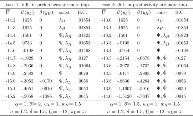
To offer some examples of the situations we have theoretically derived and shed further light on the properties of optimal policies, we conduct some numerical exercises.

Table 1 shows how policies vary when U is reduced, holding U fixed. The values of all

parameters are presented at the bottom of each table. The values of these parameters do not aim at realism, and the exercises are only for illustrative purposes. For u(·) we have used the specification u(c)≡c1−σ_{/(1−σ) in all our exercises.}

Marginal tax rates faced by the least and most productive agents are shown in columns labeledθ(yL) andθ(yH), respectively. The next column, labeledconst. presents

all the constraints that bind at the optimum through their Lagrange multipliers. Con-straints which associated Lagrange multipliers are not shown are slack at the opti-mum. Finally, the encouragement or discouragement of human capital is presented as the ratio of h(α) to the choice human capital that arises from solving the first

or-der condition with respect to h at the optimal contract. That is, the column displays

h(α)hP

iπi(yi(α)/wi)δ

i−1/2δ

−1.

When Ψ is not displayed in column labeled const., the allocation is interim efficient and we have a typical mirrleesian solution with positive marginal income taxes for the low productivity lazy and zero marginal taxes for the most productive agent. It is also possible to observe that human capital is encouraged in those circumstances, as

predicted by da Costa and Maestri (2007). When, however, Ψ > 0, the marginal tax

rate on the most productive lazy is also positive, and we provide an example where agents are bunched (λH, λL > 0) in which case human capital is not distorted at the

optimum.

5

Hard Worker’s Allocation

As in the case of Lazy agents’ our first result is a characterization of off-equilibrium behavior by lazy who announce to be hard worker.

Lemma 2 If differences in preferences for leisure are more important than differences in productivities, off-equilibrium lazy agents always announce to be of low

productiv-9

ity. When differences in productivities are more important, low productivity lazy agents strictly prefer and high productivity lazy agents weakly prefer low productivity hard worker’s bundle.

A low productivity lazy never chooses the allocation intended for the high produc-tivity hard worker. As for the most productive lazy, when differences in producproduc-tivity are more important, we cannot rule out the possibility that, off-equilibrium, she is in-different between the allocations of the two hard workers: the set defined in (2) is not a singleton. In dealing with the possibility that the agent may be indifferent between the two allocations, we must define an incentive constraint for each strategy in the set. The multiplier Ψ is then associated with the strategy of always announcing to be of low pro-ductivity while the Lagrange multiplier ˆΨ is associated with the truthful announcement of productivities by an off-equilibrium high productivity lazy.

Marginal Income Taxes According to lemma 2, the strategy of always announcing to be of low productivity is always optimal for an off-equilibrium lazy, while the strategy of announcing the true productivity may, in some cases be just as good.

Differentiating the Lagrangian with respect tocH(α), we derive the related first order

condition,

u′(cH(α)) =πH

ΦπH +λH −λL−ΨˆπH

−1

.

As for the first order condition with respect toyH(α),it is

αyH(α)

δ−1

h(α)δ_wδ H

=πH

ΦπH +λH−

α

αΨˆπH −λL wδ

H

wδ_L

−1

.

Thus, the marginal tax rate faced by the most productive hard worker, θ(yH(α)), is

θ(yH(α)) =

ˆ

ΨπH[1−α/α] +λL

h

1−(wH/wL)δ

i

ΦπH+λH −ΨˆπHα/α−λL(wH/wL)δ

≤0 (11) The first order condition with respect toyH(α) guarantees that the denominator in

(11) is positive. Both terms in the numerator are non-positive, which explains the in-equality. Because the expressions within brackets are negative,θ(yH(α)) will be negative

if either ˆΨ>0 or λL>0. In passing it is worth noting that, when ˆΨ>0 it is either the

case that agents are bunched, or,λH = 0.

A similar procedure allows us to derive the marginal income tax rate for the least productive hard worker,

θ(yL(α)) =

λH

1−(wL/wH)δ

+ Ψ1−α_απL−πH(wL/wH)δ

+ ˆΨπL

1−α_α

ΦπL−λH(wL/wH)δ+λL−Ψα_α

πL+πH(wL/wH)δ

−Ψˆα_απL

As we shall see in proposition 5 this expression can take any sign. Once again, using the fact that, absent bunching, λH = 0 if ˆΨ > 0, it is possible to show that ˆΨ > 0

implies θ(yL(α))<0.In proposition 5 we formalize this result and deal with the case

of bunching.

Proposition 5 The marginal tax rate faced by the most productive hard worker is always non-positive, while the marginal tax rate for the least productive can take either sign.

The most-productive hard worker’s allocation may be envied by agents’ whose marginal rates of substitution are steeper than the most productive hard workers’, or it may be envied by no one. In the first case, it is optimal to have negative marginal tax rates, while in the second it is optimal neither to tax nor to subsidize the agent. As for the least productive hard worker, its marginal tax rate can take any sign.

Human Capital Policy As in the case of lazy agents, the anticipation of deviant behavior by hard workers and the behavior of lazy agents who impersonate hard workers will jointly determine how human capital policies are optimally structured.

[Insert Figure 2]

An interesting thing about the hard worker’s problem, is that off-equilibrium behav-ior of lazy leads to the encouragement of human capital formation, since a lazy who announces to be hard worker works no more than the true hard worker, while the antici-pation of false announcement may drive the discouragement of human capital formation. In fact, when differences in preferences are more important and the redistributive motive, is very strong it may be optimal to transfer from the low to the high productivity agent — see figure 2, case λL>0 —, and the anticipation of false announcement will lead to

the discouragement of human capital formation. The necessary and sufficient condition for the encouragement of human capital formation to be optimal is

ΨπH

α α

wδ_L wδ

H

−λL≥0,

which, once again makes apparent the forces at play.

Proposition 6 Whenever differences in productivity are more important than differ-ences in preferdiffer-ences for leisure, human capital is (weakly) encouraged.

need to preclude lazy agents from announcing to be hard workers is operative, making the encouragement of human capital. In the second case, however, human capital should not to be distorted: if agents are bunched, hard workers and lazy agents announcing to be hard workers (trivially) behave the same way, leaving no gains from distorting choices. Along the same lines of proposition 4 we restrict the set of policies that may be justified as being optimal for some redistributive metric by showing that policies that combine disencouragement of human capital and positive marginal taxes on labor income cannot be optimal in the case of hard-workers.

Proposition 7 A policy that contemplates non-negative marginal income tax for any hard-working agent and the discouragement of human capital is inefficient.

5.1 Numerical Examples

As in section 4.1 we present some numerical exercises aimed at illustrating some of the situations presented along the section. Here, we fix the utility promise of hard workers,U and let the utility of the lazy, U , vary.

Once again, Ψ = 0, i.e., Ψ not displayed implies that allocations are interim efficient, and their qualitative properties are identical to those of interim efficient allocations of lazy agents. When Ψ>0,several interesting situations arise in our numerical exercises. First, when differences in preferences are more important, we see that it is possible to have a situation where no second period constraint binds at the optimum, e.g., when

U = −14.9.10 _{It is also possible to see that for very low values of U it is optimal to}

transfer income from the low productivity to the high productivity hard worker: an extreme form of inefficiency induced by the need to keep lazy agents from impersonating hard-workers.

The situation in which, absent bunching, a lazy is indifferent between the allocations of the two hard workers is illustrated in the second table when ˆΨ is displayed in column

const. Naturally, when this happens no second period constraint binds, yet both alloca-tions are distorted. Despite the fact that none of our tables presents bunching for the hard workers, other configurations of parameters do generate bunching at the optimum, e.g., α= 1, α= 1.5, wL= 1, wH = 1.2, σ = 1.2, δ= 1.5, U =−12, πL=.5 for values of

U below−13.55 for a grid of.025.

It is also worth mentioning the fact that in both cases we observe the sign of marginal tax rates for the least productive hard worker changing as we move from interim efficient to interim inefficient allocations.

10

Using a finer grid, 0.025????????????, we found thatλL=λH = 0 for all values ofU from -14.85

6

Implementation

In this section we describe tax implementation for the allocations derived in the

previous sections. We start by considering a tax system that works for any Pareto

efficient allocation. Then we discuss its properties questioning whether they can be dispensed with.

Define

DOM ≡ {(h, y)| ∃ (α, i) such that (h, y) = (h(α), yi(α))}.

and

DOM1≡ {h| ∃ α such thath=h(α)}

We start with the following assumption.

Assumption A: There are functions ˆc1 : DOM1 −→ R+ and ˆc : DOM −→ R+ such

that ˆc1(h(α)) =c(α) and ˆc((h(α), yi(α))) =ci(α).

This assumption is analogous to Assumption 1 in Kocherlakota (2005). It pre-cludes the possibility that two different types (α, i) and (ˆα, j) have (h(α), yi(α)) =

(h(ˆα), yj(ˆα)) whileci(α)6=cj(ˆα) or the two preference types have the same h(α) but

different c(α).

Assumption B: h(α)6=h(α).

We now consider the followingtax system. 1) Labor income tax function is

T(h, y) =

(

y−ˆc(h, y)−c(h) , if (h, y)∈DOM

2y, if (h, y)∈/ DOM .

2) Taxes on savings are

γ(h, y) =

(

1 +u′_(˜c(h))/u′_{(˜c(h, y)) , if (h, y)∈DOM}

1, if (h, y)∈/DOM .

Therefore, the budget constraint of an agent who chooses (h, y)∈DOM isc+s≤0, in the first period and c ≤ y−T(h, y) +s(1−γ(h, y)) in the second. We shall then show the following.

Proposition 8 Tax system(T, γ) implements any Pareto efficient allocation that satis-fies assumptions A and B.

outsideDOM. So we shall refrain from further discussing this aspect of the tax system. Instead we shall investigate its properties for (h, y)∈DOM.

The first property of our tax system is that labor income taxes are non-separable

between income and human capital. It is the dependence of labor income taxes on h

that commits the agent to a more restricted budget set on her productive years, and allows for a more efficient allocation—see next section. Dispensing with this dependence corresponds to allowing agents to announce her preferences in one period and choose a bundle entitled to the agent of different preferences in the second. This cannot be done, in general.11

It is due to the same reason that assumption B is needed. If the optimal allocations entails the same pair c, h for both types in the first period. Agents’ choices cannot be used to commit the agent to a second period budget set.

Taxes on savings,−c, are dependent on (h, y).Dependence on (h, y) is necessary to

avoid double deviation. Notice that we have chosen taxes that are linear in −c as in

Kocherlakota (2005). Non-linearity is not needed in our framework too.

7

The Role of Time and Uncertainty

An evolving informational set plays an important role here because some choices are made prior to agents knowing their productivities. This (potentially) allows the govern-ment to improve on what can be accomplished if no choices are made in the first period. It also creates the need to endow the government with a commitment technology. Recall that interim inefficiencies are introduced in second period bundles to handle the prob-lem of ‘lack of common knowledge of preferences’. After agents reveal their preferences, and before they realize their productivities the planner may conduct welfare improving reforms that eliminate these inefficiencies. Naturally, if agents anticipate this behavior by government, nothing will be revealed in the first period, thus reducing the scope for intertemporal tie-ins. Thus the value of commitment.

The sequential nature of learning in this setting, on the other hand, allows the planner to improve welfare. Take, for example a situation in which differences in preferences are more important then differences in productivities. In this case the ordering of the marginal rates of substitution between second period consumption and effective labor is

M RSH(α)< M RSL(α)< M RSH(α)< M RSL(α).We further assume that there are

no human capital or consumption choices to be made in the first period, which means that all possible gains will be related to the agent’s committing to a smaller second period budget set.

11

Now, imagine a social planner who maximizes the sum of expected utilities of hard workers and lazy agents subject to a given level of resources. At this point, we assume that no actions are taken in the first period: all information revelation takes place in the second period. To maximize the sum of agents expected utilities, the planner offers a mirrleesian solution easily characterized along the lines of Guesnerie and Seade (1982). At the optimum, all downward local incentive compatibility constraints bind, and the optimal allocation involves no bunching. The most productive hard worker faces a zero marginal tax on labor income, while all other agents face strictly positive marginal tax rates. Moreover, from an ex-ante perspective (before knowing her productivity), a hard worker strictly prefers the contingent budget set {yi(α), ci(α)}i=H,L to {yi(α),

ci(α)}i=H,L, while the opposite is true for lazy agents.

Let U and U denote, respectively, the expected utility attained by a hard worker

and a lazy under the mirrleesian allocation above. This allocation is also the one which minimizes the cost of delivering utilities U and U, for hard workers and lazy agents, respectively, if agents do not make choices in the first period. Now, allow the government to request a (possibly false) announcement of preferences in the first period from all agents. To each of the two possible announcement there corresponds a second period budget set, {y∗

i(α), c∗i(α)}i=H,L for a hard-worker and {yi∗(α), c∗i(α)}i=H,L for a lazy

agent. The government cannot do worse than in the previous case. We show next that it does strictly better, i.e., it delivers U , U

at a lower cost.

To see this, construct the new allocations{y∗_i(α), c∗_i(α)}i=H,Land{yi∗(α), ci∗(α)}i=H,L,

as follows {y∗

i(α), c∗i(α)} = {yi(α), ci(α)} for i = H, L, {yH∗ (α), cH∗ (α)} = {yL(α),

cL(α)}, and {yH∗(α), c∗H(α)} ≫ {yH(α), cH(α)}, where {yH∗(α), c∗H(α)} is a very

small movement along the most productive lazy’s indifference curve from point{yH(α),

cH(α)}.

This new allocation: i) is cheaper than the original one (because the most

pro-ductive lazy faces a positive marginal tax rate at point {yH(α), cH(α)}); ii) is

imple-mentable if agents are to chose between the two budget sets {y∗

i(α), c∗i(α)}i=H,L and

{y∗

i(α), c∗i(α)}i=H,L in the first period (which is guaranteed by the continuity of

prefer-ences),iii) is not implementable without the first period revelation (according to lemma 4, the least productive hard worker strictly prefers {y∗

H(α), c∗H(α)} to {yL(α), cL(α)}),

and; iv) delivers U , U

. Finally note that, at this new allocation, at least one of the budget sets (that of the hard-worker) is not envied by the other agent, which means that any leftovers could be used to increase the sum of utilities. So the reform creates room for a Pareto improvement.

fact, our cost minimization problem could, in a certain sense, be mapped into the profit maximization structure analyzed by the authors:12 _{here, the planner exerts the role of}

the monopolist, trying to extract as many resources as possible from lazy agents and hard workers, subject to incentive compatibility and promise keeping constraints, these latter constraints being analogous to the individual rationality constraints of the profit maximization framework.13

8

Conclusion

In this paper, we have considered optimal labor income taxation and human capital policies in a two period economy with heterogeneous agents.

To advance in the characterization of the problem we have adopted many simplifying assumptions about preferences and the nature of shocks. Preferences were chosen in such a way as to maintain an exogenous chain of incentive compatibility constraint despite the multi-dimensionality of the problem. Shocks were assumed to be independent of pref-erence types, which allowed us to disregard an extra source of informational advantage associated with first period deviation.

Despite all these simplifications, it is still the case that the strong results on human capital policies derived by da Costa and Maestri (2007) need not survive in this envi-ronment. While insurance aspects lead to the optimality of encouraging human capital formation, the redistributive aspects can drive policies either way. The interplay be-tween insurance and redistributive motive also implies that for some agents the sign of the marginal income tax rate will depend on the specific point in the Pareto frontier that social preferences are located.

With the exception of parts of section 6 that discusses implementation, the same forces we identify in our model will manifest themselves in a repeated Mirrlees model where agents only differ because they receive different sequences of productivity shocks throughout their lives. The results presented here in terms of the relative importance of differences in preferences vis `a vis differences in productivity would have to be reinter-preted in terms of how inequality accumulates along the life-cycle, but the same issues faced here should appear there, albeit with a little more structure.

12

It is worth mentioning, however, that in contrast with the model analyzed by Courty and Li (2000), here, agents who deviate in the first period usually pursue different second period strategies when com-pared to individuals on the equilibrium path, which makes things slightly more complicated. [COMMON KNOWLEDGE OF PREFERENCES OVER FUTURE BUNDLES?]

13

References

[1] Albanesi, S. (2006) “Optimal Taxation of Entrepreneurial Capital with Private

Information,” NBER Working Papers 12419.

[2] Albanesi, S. and C. Sleet(2006) “Dynamic Optimal Taxation with Private In-formation,” Review of Economic Studies, 73:1-30.

[3] Brito, D., J. Hamilton, S. Slutsky and J. E. Stiglitz(1990) “Pareto Efficient

Tax Structures”Oxford Economic Papers, 42: 61-77.

[4] Courty, P. and H. Li(2000). ”Sequential Screening,”Review of Economic Studies, 67: 697-717.

[5] da Costa, C. and L. Maestri (2007) “The Risk Properties of Human Capital

and the Design of Government Policies,” European Economic Review,51: 695-713.

[6] da Costa, C. and I. Werning (2007) “On the Optimality of the Friedman Rule

with Heterogeneous Agents and Non-Linear Income Taxation” Working Paper.

[7] Fernandes, A. and C. Phelan (2000) “A Recursive Formulation for Repeated

Agency with History Dependence”Journal of Economic Theory, 91: 223-247.

[8] Golosov, M., N. Kocherlakota, and A. Tsyvinski (2003). “Optimal Indirect and Capital Taxation.” Review of Economic Studies, 70: 569-587.

[9] Golosov, M. and A. Tsyvinski (2006) “Optimal Taxation with Endogenous

Insurance Markets.”Quarterly Journal of Economics, forthcoming.

[10] Golosov, M., A. Tsyvinski and I. Werning (2006). “New Dynamic Public

Finance: A User’s Guide”NBER Macro Annual.

[11] Grochulski, B. and T. Piskorski (2005) “Optimal Wealth Taxes with Risky

Human Capital”,Richmond Federal Reserve Bank Working Paper, 05-13.

[12] Guesnerie, R. and J. Seade (1982) “Nonlinear Pricing in Finite Economies”,

Journal of Public Economics, 17: 157-179.

[13] Kapicka, M.(2006) “Optimal Income Taxation with Human Capital Accumulation

and Limited Record Keeping”Review of Economic Dynamics, 9: 612-639.

[15] Kocherlakota, N.(2005a) “Advances in Dynamic Optimal Taxation” inAdvances in Economics and Econometrics: Theory and Applications, Ninth World Congress, Vol. I, edited by R. Blundell, W. Newey, and T. Persson, Cambridge University Press.

[16] Kocherlakota, N. (2005b) “Zero expected wealth taxes: a Mirrlees approach to

dynamic optimal taxation.”Econometrica, 73: 1587-1621.

[17] Malcomson, J. and F. Spinnewyn (1988) “The Multi-period Principal-Agent

Problem”,The Review of Economic Studies, 55: 391-408.

[18] Mirrlees, J.(1971) “An Exploration in the Theory of Optimum Income Taxation”,

The Review of Economic Studies, 38, 175–208.

[19] Rochet, J-C. and L. Stole (2003) “The Economics of Multidimensional

Screen-ing” inAdvances in Economics and Econometrics: Theory and Applications, Eight

World Congress, Vol. I, edited by M. Dewatripont, L. Hansen and S. Turnovsky, Cambridge University Press.

[20] Stiglitz, J. E. (1982) “Self-selection and Pareto Efficient Taxation,” Journal of Public Economics, 17, 213-240.

A

Appendix

Lemma 3 First period bunching is never optimal.

Proof. First, notice that if differences in preferences are more important, first period bunching is only possible if agents are also bunched in the second period, i.e., yH(α) =

yH(α) =yL(α) = yL(α).This cannot be the case, as we shall prove later. So, assume

that differences in productivities are more important. We start by remarking that, under first period bunching, yi(α) = yi(α), i = H, L yet, θ(yi(α)) > θ(yi(α)), i = H, L.

Assume that second period upward IC is slack. I first argue that θ(yH(α)) cannot

be positive. Were it the case, then, increasing yH(α) along the indifference curve of

(α, H) agent, utility would be preserved and resources saved. So, assume θ(yH(α))≤0

then θ(yH(α))<0.Then, reducingyH(α) indifference curve will save resources and is

incentive compatible. So upward constraint must bind. Next, assume that the downward constraint is slack. We know that θ(yL(α)) > θ(yL(α)) if θ(yL(α)) > 0, slightly

increasingθ(yL(α)) along (α, L) indifference curve saves resources and preserves utility.

If, on the otherθ(yL(α))≤0,θ(yL(α))<0. ReducingyL(α) along (α, L)’s indifference

Then it must be the case that either θ(yH(α)) > 0 or θ(yL(α))< 0.In both cases a

welfare-preserving reform saves resources.

Proof of lemma 1. The result is trivial in case of bunching. Without bunching, if the allocation is implementable,

u(cH(α))−u(cL(α)) ≥ α

δ

yH(α)

h(α)wH

δ"

1− yL(α)

δ

yH(α)δ

#

=⇒ (12)

u(cH(α))−u(cL(α)) >

α δ

yH(α)

h(α)wH

δ"

1− yL(α)

δ

yH(α)δ

#

. (13)

due to monotonicity. The last inequality shows that high productivity hard workers strictly prefer the allocation of high productivity lazy agents.

For the low productivity hard worker, we consider two cases separately: i) if differences in preferences are more important, α/w_Hδ > α/w_Lδ, and (12) implies

u(cH(α))−u(cL(α))>

α δ

yH(α)

h(α)wL

δ"

1− yL(α)

δ

yH(α)δ

#

,

thus proving the result; ii) if differences in productivities are more important, assume that the low productivity hard worker weakly prefers the allocation intended for the most productive lazy, that is

u(cH(α))−u(cL(α))≥

α δwδ

1

yH(α)

h(α)

δ"

1− yL(α)

δ

yH(α)δ

#

. (14)

If α/wδ_H < α/w_Lδ equation (14) implies

u(cH(α))−u(cL(α))>

α δwδ

2

yH(α)

h(α)

δ"

1− yL(α)

δ

yH(α)δ

#

,

i.e., both second period incentive compatibility constraints are slack. Reducing cH(α)

and increasing cL(α) so as to maintain unchanged the expected utility for lazy agents,

does not change the expected utility of deviant hard workers, thus preserving incentive compatibility. Monotonicity and strict concavity ofu(·) guarantees that the reform saves resources. A contradiction.

Lemma 4 For any two agents, iand j, ifM RSi> M RSj, then:

i) for two allocations (c, y) and (ˆc,yˆ) with (c, y) ≪ (ˆc,yˆ) if agent j weakly prefers allo-cation (c, y), agent istrictly prefers (c, y)

Proof. Single-crossing implies that the ranking of marginal rates of substitution is independent of the specific allocation we consider. From here, the proof is trivial.

Proof of Proposition 1. If the first period constraint is slack, the second period problem is just a traditional two agent Mirrlees’ problem. The first two properties are derived, for example, in Stiglitz (1987). As for the third, when constraint Ψ is slack, our problem is a particular case of that examined in da Costa and Maestri (2007), where a simple proof can be found.

Lemma 5 The constraint that prevents the high productivity lazy from mimicking the low productivity is always binding at the optimum.

Proof. Trivial in case of bunching. Absent bunching, assume the lemma is not true. Reducing cH(α) a little and increasing cL(α) proportionately so as to maintain

the expected welfare of lazy agents reduces cost due to monotonicity and strict concavity of u(c(α, w)). Lemma 1 guarantees that incentive constraints are not violated. We have found another implementable allocation which is cheaper than the optimal one. An absurd.

Proof of Proposition 2. First, consider the case in which lazy agents are bunched at allocation (y∗_{, c}∗_{). If at least one lazy faces a strictly negative marginal income tax}

rate this must be the case for the least productive lazy. Now, consider an alternative allocation (ˆy,ˆc) where (ˆyH(α),ˆcH(α)) = (y∗, c∗), while (ˆyL(α),ˆcL(α))≪(y∗, c∗) is in the

same indifference curve of the low productivity agent as (y∗_{, c}∗_{). According to lemma}

4, (ˆy,ˆc) keeps everyone’s welfare unchanged (both deviant hard workers will choose (ˆyH(α),cˆH(α)) under this new scheme), meaning that the new allocation is incentive

compatible. If the least productive lazy faces a strictly negative marginal income tax rate at (y∗_{, c}∗_{), the new allocation saves resources for (ˆy,cˆ) close enough to (y}∗_{, c}∗_).

This contradicts the optimality of (y∗_{, c}∗_{), therefore the marginal tax rate on the least}

productive lazy is non-negative. The ranking of marginal rates of substitution guarantees that the marginal tax rate for the most productive lazy is strictly positive in this case. Absent bunching, the case in which differences in preferences are more important was considered in the text, we shall then consider the opposite case. Lemma 5 shows that the constraint that prevents the most productive agent from pretending to be the least productive one binds which implies that the other constraint is slack. The first order condition with respect toyL(α) is

πL=α

yL(α)δ−1

h(α)δ

nh

ΦπL−Ψ

α α

i

wδ_L−λHw−_Hδ

Substituting wLfor wH and α forα we get

πL> α

yL(α)

h(α)wL

δ

ΦπL−λH −ΨπL

yL(α)

Using the first order condition with respectcL(α), πL= (ΦπL−λH −ΨπL)u′(cL(α)),

this inequality implies

α wLh(α)

yL(α)

wLh(α)

δ−1

< u′(cL(α)).

The marginal income tax rate for the least productive lazy is positive. Now, consider the first order condition with respect to yH(α),

πH =

h

ΦπH+λH −Ψα

απH

i α

wHh(α)

yH(α)

wHh(α)

δ−1

.

Substituting α forα, we get

πH >[ΦπH +λH −ΨπH]

α wHh(α)

yH(α)

wHh(α)

δ−1

which, usingπH = [ΦπH +λH −ΨπH]u′(cH(α)) yields

α wHh(α)

yH(α)

wHh(α)

δ−1

< u′(cH(α));

a positive marginal income tax rate for the most productive lazy.

Proof of Proposition 3. With bunching, the first order condition with respect to

h(α) is

h(α)δ−1−h(α)−δ−1y(α)δX

iπiw

−δ i

(Φα−Ψα) = 0.

Also, Φα−Ψα > α(Φ−Ψ) = αu′_(c(α))−1 _{> 0. Therefore, h(α)}2δ _{= y(α)}P

iπiw−i δ,

so if there is bunching human capital is not distorted. Absent bunching, whenever differences in productivities are more important, off-equilibrium hard workers tell the truth aboutwin the second period (lemma 1). Therefore, the first order condition with respect to human capital is

h(α)δ−1−X

iπi

yi(α)

wih(α)2

yi(α)

wih(α)

δ−1

= λHα

(Φα−Ψα)h(α)

yH(α)

wHh(α)

δ"

1− yL(α)

δ

yH(α)δ

#

.

Since the term Φα−Ψαis positive, so is the right hand side of the expression. The private marginal cost of acquiring human capital is higher than its expect marginal benefit.