www.hydrol-earth-syst-sci.net/14/447/2010/ © Author(s) 2010. This work is distributed under the Creative Commons Attribution 3.0 License.
Earth System
Sciences
Selection of an appropriately simple storm runoff model
A. I. J. M. van Dijk
CSIRO Land and Water, Canberra, ACT, Australia
Received: 12 August 2009 – Published in Hydrol. Earth Syst. Sci. Discuss.: 9 September 2009 Revised: 12 February 2010 – Accepted: 15 February 2010 – Published: 8 March 2010
Abstract. An appropriately simple event runoff model for catchment hydrological studies was derived. The model was selected from several variants as having the optimum balance between simplicity and the ability to explain daily obser-vations of streamflow from 260 Australian catchments (23– 1902 km2). Event rainfall and runoff were estimated from the observations through a combination of baseflow separation and storm flow recession analysis, producing a storm flow recession coefficient (kQF). Various model structures with up
to six free parameters were investigated, covering most of the equations applied in existing lumped catchment models. The performance of alternative structures and free parame-ters were expressed in Aikake’s Final Prediction Error Cri-terion (FPEC) and corresponding Nash-Sutcliffe model ef-ficiencies (NSME) for event runoff totals. For each model variant, the number of free parameters was reduced in steps based on calculated parameter sensitivity. The resulting opti-mal model structure had two or three free parameters; the first describing the non-linear relationship between event rainfall and runoff (Smax), the second relating runoff to antecedent
groundwater storage (CSg), and a third that described initial
rainfall losses (Li), but which could be set at 8 mm
with-out affecting model performance too much. The best three parameter model produced a median NSME of 0.64 and out-performed, for example, the Soil Conservation Service Curve Number technique (median NSME 0.30–0.41). Parameter estimation in ungauged catchments is likely to be challeng-ing: 64% of the variance in kQF among stations could be
explained by catchment climate indicators and spatial corre-lation, but corresponding numbers were a modest 45% for
CSg, 21% forSmaxand none forLi, respectively. In gauged
catchments, better estimates of event rainfall depth and in-tensity are likely prerequisites to further improve model per-formance.
Correspondence to:A. I. J. M. van Dijk ([email protected])
1 Introduction
Estimating catchment streamflow where or when it is not ob-served is a well established field of hydrological research (e.g. Sivapalan et al., 2003). Accurate prediction requires an appropriate model structure and methods to estimate model parameters. There is a well-known trade off between, on one hand, using a simple model that does not describe the avail-able data well and, on the other, using a complex model that contains too many similar equations to reliably estimate their parameters (the ’‘equifinality” problem; Beven, 1993).
This study revisits the question posed by Jakeman and Hornberger (1993): “How much complexity is warranted in a rainfall-runoff model?”. However, where those authors fo-cused on the number of linear or parallel stores that best de-scribed the delayed release of water from a catchment, the current study focuses on the optimal functional form of the set of equations used to estimate what part of event precipi-tation is converted into storm runoff. The scope of this study is limited to hydrological models with process equations that operate on a daily time step and describe the behaviour of catchments rather than (segments of) hillslopes. Many such so-called ‘lumped’ models have been proposed (reviewed in e.g. Beven, 2004; Bl¨oschl, 2005; Maidment, 1992) and are widely used as a comparatively parsimonious, pragmatic ap-proach to estimating streamflow generation under historic, scenario or forecasted conditions.
Reflecting this ambiguity, the various existing rainfall-runoff models make different, often implicit, assumptions about the significance or insignificance of alternative runoff processes. A generic set of equations that captures most thresholds and variables may be:
R=fsatPn+(1−fsat)Pn−I+Rreturn (1)
Pn=max(0,P−Li)=(1−fn)P (2)
I=fIPn (3)
Rreturn=(1−fs)I (4)
whereRis runoff, Pn net rainfall,I net infiltration into the
soil, Rreturn return flow from the soil (all in mm per event
or mm d−1), andfsat the fraction saturated area. Pn is
of-ten expressed as total rainfall less an initial loss Li (mm)
which may be conceptualised as a constant or a proportion
fn(or a combination of both) and assumed to represent
infil-tration and/or evaporative losses. The fractionfI represents
the fraction of net rainfall on unsaturated soil that infiltrates, andfs the fraction ofI that can be retained in the soil.
This generalised model is usually simplified one way or another, for example, by assuming that fsat, fn, fI or fs
are either negligible or equal to unity (e.g. Bergstr¨om, 1992; Chiew et al., 2002). It may also be made more complicated by introducing further functional relationships, for example expressingfsatas a function of groundwater level or storage,
or expressingfI as a function of storm size or rainfall
inten-sity and/or soil water content, or expressingfsas a function
of actual and maximum soil water storage. Additionally, one or several of the variables in these equations may be repre-sented by spatial distribution functions, for example to rep-resent sub-grid variability in coarse resolution land surface models (e.g. Bonan, 1996; Liang et al., 1994; Liang and Xie, 2001; Oleson et al., 2004). Each addition introduces further assumptions and, importantly, model parameters.
An illustration of the ambiguity in model interpretation due to the multitude of equivalent storm runoff processes is provided by considering the widely used Soil Conserva-tion Service Curve Number method (SCS-CN; USDA-SCS, 1985). It can be recast in a form somewhat similar to Eq. (1) as:
R=Pn
Pn
Pn+S
(5) WhereS is notionally the maximum retention after runoff begins (mm). The SCS-CN model was derived empirically however, and when comparing the second term of Eq. (5) to Eqs. (1–4) it can be interpreted in several ways:
– Equivalent to (1–fn), representing the functional
rela-tionship between storm size and fraction rainfall in ex-cess of infiltration capacity, in which casePncould be
interpreted as a proxy for rainfall intensity andS as a proxy for maximum infiltration rate (whilefsat= 0 and
fs= 0).
– Equivalent to (1–fs), representing the functional
rela-tionship between storm size and return flow fraction, in which caseSrepresents maximum soil storage capacity (whilefsat= 0 andfI= 1).
– Equivalent tofsat, representing a functional relationship
between storm size and saturated catchment area that could arise if cumulative infiltration or run-off/run-on processes lead to increase of the saturated area over the course of a storm, wherePnmight be a proxy for cumu-lative infiltration or actual runoff, andSa proxy of the efficiency of soil and catchment drainage (in which case
fn= 1 andfs= 0).
Elaborations of the SCS-CN method that implicitly or ex-plicitly assume one of these three underlying explanations (or a combination) do exist, for example by relatingSto land cover or soil conditions, or by modifyingS as a function of antecedent rainfall or groundwater storage (for examples of both see Maidment, 1992; Mishra and Singh, 2003). Pre-sumably the effectiveness of these elaborations will depend on dominant runoff processes.
The same point could have been demonstrated with other lumped runoff models, but this study does not attempt to ad-dress the ambiguity in interpreting models, which requires field study. However, the examples given emphasise the risks in increasing model complexity (adding processes, equa-tions, parameters) without a solid justification through im-proved model performance. To date, there does not appear to have been a comprehensive and formal statistical analy-sis to assess what is an appropriately simple model to de-scribe the relationship between event precipitation and event runoff at catchment scale. Since dominant runoff processes are expected to vary between catchments of different sub-strate, climate and land use, it would be anticipated that dif-ferent model structures may perform better in difdif-ferent catch-ments.
The aims of the study were as follows:
– Test several alternative versions and simplifications of the generalised storm flow model expressed in Eq. (1) for their performance in reproducing estimated event storm flow from 260 catchments across Australia. – Assess the appropriate balance between the number of
free parameters and model performance, by considering an information criterion as well as correlation between different parameters that may be indicative of equiva-lence.
– Assess to what extent model parameters can be pre-dicted in ungauged catchments from catchment at-tributes and spatial correlation.
0 250 500 1,000km streamflow stations
rain gauges
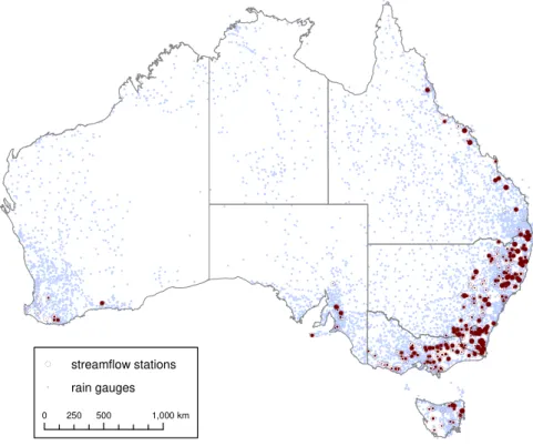
Fig. 1.Map showing the location of the stations for which data were analysed. The relative size of the inner dot corresponds to the Nash-Sutcliffe model efficiency (attained with the best three-parameter model and corrected for the number of free parameters). The distribution of gauges underpinning the interpolated rainfall product is indicated (for an arbitrary day in 2005).
2 Methods
2.1 Data
Daily streamflow data (in ML d−1) were collated for 362 catchments across Australia as part of previous studies (Peel et al., 2000; Guerschman et al., 2008, 2009). Streamflow data for these selected catchments were considered of satis-factory quality and any influence of river regulation, water extraction, urban development, or other processes upstream considered unimportant. Large lakes or wetlands do not oc-cur in any of the catchments, but smaller impoundments can occur. From the data set, those records were selected that had good quality observations for at least five years during the pe-riod 1990–2006 and no less than 50 runoff events (defined as an increase in streamflow from one day to the next).
The selected 260 stations were located in southwest West Australia, Tasmania, and coastal regions of the eastern states (Fig. 1). The contributing catchments of all gauges were de-lineated through digital elevation model analysis and visual quality control. Catchment areas varied between 23–1902 (median 333) km2.
Daily streamflow volumes were converted to streamflow depths (Q, mm d−1) and varied from 2 to 1937 (median 114) mm y−1. Catchment-average daily precipitation was calculated using a gridded 0.05◦ precipitation product
de-rived by interpolation of station data (Jeffrey et al., 2001). Of the rain gauges used in interpolation, on average there were three (range 0–22) inside or within 5 km of each catchment. The range of average annual rainfall for the catchment sam-ple was 317–2983 (median 851) mm y−1; precipitation other than rainfall was not important. Priestley-Taylor potential evapotranspiration (E0) was 651–2417 (1254) mm y−1 and
catchment humidity (H, the ratio of average rainfall over av-erageE0) was 0.13–3.48 (0.68). The data set includes
catch-ments under native forest, catchment fully cleared for graz-ing, and catchments with a varying combination of croppgraz-ing, grazing, plantation forestry and native vegetation.
2.2 Streamflow analysis
The streamflow data were separated into time series of daily estimated baseflow (BF orQBF) and quick flow (QF orQQF)
by combining forward and backward recursive linear reser-voir baseflow filter as described in Van Dijk (2010). It was assumed that the estimated QF represents the sum of all storm runoff processes and BF the delayed groundwater dis-charge, but it is noted that the hydrograph per se cannot pro-vide epro-vidence for this interpretation.
from the storm flow time series, all days t=i showing a storm flow peak were identified, that is, all days for which
QQF(i–1)<QQF(i) > QQF(i+1). For each station a weighted
average storm flow recession constant was calculated follow-ing the theory for a linear store (cf. Van Dijk, 2010) as:
kQF= −ln
PQ
QF(i+1)
P
QQF(i)
(6)
Total event rainfallP (i)for the event peaking on day t=i
was subsequently estimated as:
Pev(i)= i
X
t=i−2
P (7)
wheret=i−2 was chosen to account for the fact that the recorded rainfall event and the peak in storm flow were oc-casionally separated by up to two days due to the different times of rainfall and streamflow recording (09:00 a.m. and 24:00 p.m., respectively). Total event runoffR(i)was esti-mated as:
R (i)=
tn
X
t=i−2
QQF+SR(tn) (8)
=
tn
X
t=i−2
QQF+
QQF(tn+1)
1−exp −kQF
wheretnis the day on whichQQF(tn) is ten times less than QQF(i). This was done to avoid inclusion of storm runoff
from subsequent rainfall events. The termSR(tn) is the
esti-mated storm runoff still in storage at the end of daytnbased
on linear reservoir theory.
Several studies have found that runoff response is positively related to groundwater level measurements in piezometers and antecedent streamflow rates (e.g. Dunne and Black, 1970) and this was also observed for several Aus-tralian catchments (e.g. Liu et al., 2007; Pe˜na Arancibia et al., 2007; Beck et al., 2010). This is commonly attributed to the growth of saturated areas as groundwater rises. To al-low inclusion of this correlation in the model, groundwater storageSgwas estimated from the daily baseflow (QBF)
es-timates as:
Sg(i)=
QBF(i)
1−exp(−kBF)
(9)
wherekBFis the baseflow recession constant. Values ofSg
on the first day of each runoff event were used as an estimate of antecedent groundwater storageSg(i)before runoff event i. Due to the method of baseflow separation these values were estimated from the preceding baseflow recession with a forward filter and therefore not influenced by the storm flow event itself (cf. Van Dijk, 2010).
2.3 Evaluation of alternative model structures
For each of the model variants that was tested, the most com-plex model (that is, the one with the maximum number of pa-rameters) was gradually simplified based on parameter sen-sitivity analysis, and the corresponding change in prediction error was calculated. The basic model structure tested had the form (cf. Eqs. 1–4):
Pn=max(0,P−C1) (10)
R=
"
(C2Pn)C3 Pn+C4
#
Pn (11)
whereC1,C2,C3andC4are all optionally free parameters.
Each of these parameters can be effectively omitted by giv-ing it a value of either zero or unity. For example,C4= 0
sim-plifies the equation to a power function ofPn, while in addi-tionC3= 1 produces a constant runoff fraction, andC1= 0
re-moves the rainfall threshold before runoff is produced. With
C3= 1 andC2=1 the equation mirrors the SCS-CN model. To
test whether model performance was further improved if the model took into account the effect of antecedent groundwater storageSgthe following modifications were also tested:
R= (C2Pn)
C3
Pn+C4
(1−fsat)+fsat
!
Pnwith (12)
fsat=max
1,C5SgC6
and
R=
"
(C2Pn)C3 Pn+Smax
#
Pnwith (13)
Smax=C4min
0,1−C5SgC6
whereC5andC6are again parameters that could be fitted or
prescribed values of zero or unity. It follows that the most complex models had six free parameters.
To assess the trade-off between the number of free model parameters and the improvement in model performance, Akaike’s Final Prediction Error Criterion (FPEC; Akaike, 1970) was used. FPEC represents the expected prediction error that would result were the model tested on a different data set, and is calculated as the product of the prediction er-ror (ε) and a penalization factor that considers the degrees of freedom (d, the number of free parameters) in comparison to the number of observations (n):
F P EC=1+d
n
1−d
nε (14)
The errorεwas estimated as the mean squared error between observed and modelled event runoff estimates. It was found by optimising the free model parameters with minimum ε
to find a near-optimal parameter set for each model variant. The number with draws was 10d(but with a minimum of 102 and a maximum of 104), after which the optimal parameter set was found with a Nelder-Mead Simplex search.
The value ofn was calculated as the number of rainfall events used to fit the model. In principle, the model with the lowest FPEC should be adopted. However, Schoups et al. (2008) pointed out that Eq. (14) assumes thatn≫d and may lead to underestimates of prediction error and favour overly complex models. This caveat was considered when interpreting FPEC values. Nash-Sutcliffe model efficiency (NSME; Nash and Sutcliffe, 1970) is arguably the most com-mon metric to express runoff model performance in calibra-tion (despite some undesirable properties; Legates and Mc-Cabe, 1999; Criss and Winston, 2008). As it can be calcu-lated from the mean squared error, an adjusted NSME for prediction could be calculated from the FPEC and was used in interpretation.
Another factor to consider in deciding the optimal model structure was correlation between fitted parameters, with high correlations being indicative of parameter equivalence. The parametric and non-parametric (ranked) coefficient of correlation (randr∗, respectively) between fitted parameters was considered an indicator of possible equivalence between model parameters.
2.4 Spatial predictors of model parameters
The procedure described in Van Dijk (2010) was used to as-sess the predictability of calculated values of kQF and the
fitted parameter values of the optimal model. The anal-ysis involved statistical analanal-ysis of parameteric and non-parameteric correlation coefficients (randr∗) with a variety
of catchment attributes, including catchment geology; mor-phology (size, mean slope, flatness); soil characteristics (sat-urated hydraulic conductivity, dominant texture class value, plant available water content, clay content, solum thickness); climate indices (P,E0,H, remotely sensed actual
evapotran-spiration, average monthly excess precipitation); and land cover characteristics (fraction woody vegetation, fractions non-agricultural land, grazing land, horticulture, and broad acre cropping, remotely sensed vegetation greenness). Fol-lowing this correlation analysis, any spatial correlation in the residual variance was analysed by fitting semi-variograms. Further details on the data sources and procedures can be found in Van Dijk (2010).
3 Results
3.1 Optimal model structure
The average station record included 2178 storms (range 691– 3734). Of these, 19% (2–51%) produced storm flow, result-ing in an average 631 (30–1005) events. The reduction in prediction error that is required to accept another parameter
is influenced by the definition ofnin Eq. (14). The number of observed runoff events was used here, implying that on av-erage an improvement of 0.32% would be required for an ad-ditional parameter to be accepted. Had the number of rainfall events been used instead, the improvement would only need to be 0.09% on average. Conversely, however, typically only some 10 to 20 events produced the large majority of runoff and variance in the runoff (Fig. 4a); if this number had been used instead the improvement would need to be in the order of 10–20%.
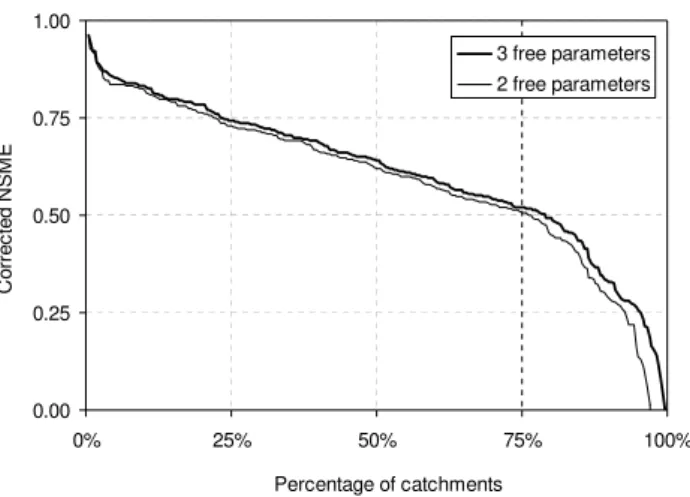
The best results obtained with all model variants using be-tween six and one parameter are listed in Table 1. Equa-tion (12) provided the best results among the alternative model structures tested. Table 1 suggests that the six pa-rameter model has the best predictive power, but for reasons mentioned this small difference is not a robust result. Model performance appeared to remain very similar as the number of fitting parameters was reduced to three. FPEC increased slightly as the number of parameters was reduced to two (by 0.2% and 4.1% in median and mean FPEC, respectively), but increased much more if the number of parameters was fur-ther reduced to one. The two- and three-parameter model variants produced similar NSME values (Table 1; based on calculated FPEC and hence also allowing for the number of free parameters). The main differences occur for catchments with overall low model performance (Fig. 2).
An interpretative notation for the three and the two param-eter version of Eq. (12) could be:
R=
P
n Pn+Smax
(1−fsat)
Pn (15a)
with
Pn=max(0,P−Li) (15b)
and
fsat=max(1,CSgSg) (15c)
whereSmax(mm) is maximum storage capacity,Li(mm)
ini-tial loss, and CSg (mm−1) saturated area coefficient. The
definition of Smax is similar but slightly different from the
SCS-CN model (Eq. 5).
3.2 Parameter values and predictability
Correlation among parameters decreased as the number of free parameters was reduced. For the six-parameter model, the highest absolute value ofr(r∗) between parameters was
0.39 (0.40), and gradually reduced to 0.29 (0.25) for the three parameter model, and 0.12 (0.04) for the two param-eter model, respectively. The highest correlation in the three parameter model was between optimised values of Li and CSg; correlation withSmaxwas small (|r|<0.15).
Table 1.Change in predictive model performance as the number of free parameters is reduced from six to one. Listed are Final Prediction Error Criterion (FPEC) and adjusted Nash-Sutcliffe Model Efficiency (NSME) calculated from it. All values relate to the best performing model structure.
Number of model parameters
six five four three two one
median FPEC (mm) 0.91 0.93 0.92 0.93 0.93 1.43
mean FPEC (mm) 1.49 1.52 1.52 1.52 1.58 2.52
mean NSME 0.64 0.62 0.62 0.61 0.49 −4.11
median NSME 0.66 0.64 0.64 0.64 0.61 0.43
variance-weighted NSME 0.68 0.67 0.67 0.67 0.62 0.03
Table 2. Descriptors of the distribution in parameters of the preferred model variants: the storm flow recession coefficientkQF(d−1)
calculated directly from the observations, and optimised model parameters initial lossLi(mm), maximum storage capacitySmax(in 103mm), and saturated area coefficientCSg(in 10−3mm−1).
Symbol kQF Li Smax CSg
Unit – mm 103mm 10−3mm−1
Median 0.76 7.68 1.34 16.16
Mean 0.77 16.41 16.54 31.69
CV 31% 151% 207% 138%
25–75% range 0.60–0.91 2.71–18.93 0.53–4.3 5.27–38.29 10–90% range 0.49–1.08 0–41.44 0.25–100 1.17–72.95
0.00 0.25 0.50 0.75 1.00
0% 25% 50% 75% 100%
Percentage of catchments
Co
rr
e
c
te
d
NS
M
E
3 free parameters 2 free parameters
Fig. 2. Cumulative distribution of Nash-Sutcliffe model efficiency (NSME) for the model variants with three and two free parameters, respectively.
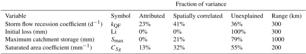
The amount of variance between stations that could be ex-plained by catchment attributes and the fraction of residual variance that was spatially correlated are listed in Table 3.
Values of kQF showed correlation with catchment
cli-mate indicators, such as average monthly excess precipita-tion (AMEP,r∗=−0.52), potential ET (E0,r= 0.50) and
hu-midity (H, r∗=-0.49), and some correlation with the
frac-tion of catchment under non-agricultural cover (r∗=−0.45).
The highestkQF values (i.e. fastest recessions) occurred in
dry catchments. The strongest regression equation was a lin-ear function ofE0, explaining 23% of the variance. Another
41% of the variance was spatially correlated over distances of ca. 300 km; the remaining 36% of variation was left unex-plained (Table 3).
None of the catchment attributes correlated withLi and a predictive regression equation could not be established. The strongest correlation found was with depth-averaged rainfall intensity (r∗= 0.31). There was also no obvious spatial cor-relation.
Similarly, no catchment attribute correlated with Smax.
The strongest correlation found was with the coefficient of variation in monthly rainfall (r∗= 0.33). About 21% of the variance in (log-transformed) Smax values appeared
corre-lated over lengths of 1000 km or more.
Finally, the saturated area coefficient CSg in mm−1
Table 3.Summary of the analysis of variance in parameter values derived from fitting the optimal runoff model to event runoff estimates from the 260 catchments. Listed are the fraction of variance explained by catchment attributes, the residual variance showing spatial correlation and the remaining unexplained variance. Also listed are the range (km) of the fitted semi-variograms.
Fraction of variance
Variable Symbol Attributed Spatially correlated Unexplained Range (km)
Storm flow recession coefficient (d−1) kQF 23% 41% 36% 300
Initial loss (mm) Li 0% 0% 100% 300
Maximum catchment storage (mm) Smax 0% 21% 79% 1000
Saturated area coefficient (mm−1) CSg 13% 32% 55% 200
4 Discussion
4.1 Optimal storm runoff model structure
Based on the calculated FPEC values alone, the six-parameter model could be accepted as theoretically having the smallest prediction error. However, the deterioration in performance between the six- and three-parameter model seems insignificant when considering that the FPEC likely was too lenient on additional parameters. Among the re-maining three parameters,Li appeared the least necessary
parameter. Mean FPEC increased by 4% if the median fit-tedLi value (8 mm) was used. Together with the apparent
lack of predictability ofLi (no correlation with catchment
attributes or spatial correlation could be found), this may not be enough basis to prefer the three-parameter model over the two-parameter variant. Reducing the number of parameters to one strongly deteriorated performance.
The SCS-CN technique is one of most widely used mod-els to estimate event runoff, and shows some similarities with the optimal model structure derived here. Therefore a direct comparison of performance is of interest. Following an oth-erwise identical approach, two commonly used versions of the SCS-CN model were fitted to the event rainfall and runoff estimates. The two parameter version with initial lossIa(in SCS-CN notation, equivalent toLi) and maximum storage S (equivalent toSmax) produced a mean FPEC of 1.82 mm
and a median NSME of 0.41. The values ofIaandSwere
slightly negatively correlated (r=−0.20) rather than show-ing the positive correlation expected (cf. Maidment, 1992; Mishra and Singh, 2003; USDA-SCS, 1985). Converting the optimisedSto curve numbers produced CN values that were beyond the recommended range of 30–100 for 80 out of 260 stations. Fitting the one-parameter version, where it is as-sumed that Ia= 0.2S, produced a FPEC of 1.80 mm and a
median NSME of 0.30. Converting the optimisedSvalues to curve numbers suggested an average CN of 60 (standard de-viation±12), and CN values were within the recommended range for 255 out of 260 stations.
It is concluded that the optimal two-parameter model se-lected outperforms the SCS-CN method by 14–15% when
considering the mean FPEC (1.58 vs. 1.80–1.82) and more so when considering the median NSME (0.61 vs. 0.30–0.41). Therefore, at least for Australian conditions, Eq. (16) appears an improvement when compared to the SCS-CN technique, or indeed any of the other storm runoff modelsthat can be expressed in terms equivalent to (12) or (13). Because the main difference with the SCS-CN technique is the consider-ation of groundwater storage dependent runoff response, it follows that antecedent wetness conditions have demonstra-ble predictive potential (cf. Beck et al., 2010).
4.2 Storm flow recession coefficient
Most catchments showed storm flow recession ‘half times’ of about one day (kQF= 0.77 d−1) with the most rapid drainage
in dry catchments. This is consistent with the expectation that storm flow under dry conditions would be predominantly through infiltration excess overland flow during a small num-ber of high intensity rainfall events. The 260 catchments var-ied considerably in size (23 to 1902 km2) and because of as-sociated differences in runoff travel time a relationship with catchment size might have been expected. Regression anal-ysis did not indicate any such relationship (r= 0.20). Pub-lished methods to estimate surface travel times (Maidment, 1992) produce travel times between<0.05 day to ca. 0.5 day for the catchment size range, and ca. 0.1 days for the median 333 km2catchment. Compared to the derived recession half times of around one day these numbers are small, and there-fore it appears overland and channel storm flow routing is not the main cause for the observed storm flow recessions. It is concluded that storm flow recession is likely dominated by the release of water that is temporary retained in the catch-ment (e.g. in ephemeral water bodies, draining soil or fast responding groundwater).
4.3 Initial loss
initial abstraction equals 0.2 of maximum retention (USDA-SCS, 1985) and combining this with curve number estimates of 60 to 90 (covering most of the range recommended for for-est and grazing land) produces initial abstraction for-estimates of 6–34 mm.
Optimal values ofLi could not be predicted, but an ini-tial loss of 8 mm caused little deterioration in model perfor-mance. Trialling alternative values forLi suggested that
val-ues of 6–12 mm produced the best FPEC, but FPEC deterio-rated by less than 2% for any value between zero and 19 mm. Initial losses are a conceptual water balance component covering a variety of processes, including rainfall retained by vegetation canopy and other surfaces and subsequently evaporated (typically in the order of 1–3 mm; e.g. van Dijk and Bruijnzeel, 2001), losses to wet up a dry soil Surface, and runoff retained in surface depressions that need to be filled before catchment runoff occurs (technically not an initial loss but likely to be lumped into it due to the model structure). 4.4 Maximum storage capacity
Between the three- and two-parameter model versions, the optimisedSmax values changed by more than 20% for 41%
of stations. It is concluded that this parameter is rather poorly constrained. Values ofSmaxfound through optimisation were
generally very high: 74% of stations had fitted values of more than 600 mm, and the maximum bound set at 105mm was still suboptimal for 9% of stations. Such high values make interpretation as a ‘maximum potential retention’ unrealis-tic and call for another interpretation. When the ratioSmax
overPnattains high values, Eq. (15a) approaches the linear
relationship:
R≈
(1−fsat)
Pn Smax
+fsat
Pn (16)
For example, forSmax= 500 andPn= 50, the difference inR
calculated from Eqs. (15a) and (16) is 10%. Fitting Eq. (16) to the data led to an overall deterioration in FPEC of 0.9%. Although Eq. (16) was preferred for its more realistic limits, it may be more conceptually appropriate to rewrite it in the equivalent form:
R=
(1−fsat)
kPPn kPPn+1+fsat
Pn (17)
wherekP is a constant of proportionality that describes the
initial increase in runoff fraction with event precipitation. More than once mechanism can be invoked to explain why runoff fraction should increase with rainfall event, as implied by Eq. (17). A rapid increase of temporarily saturated surface area as more rainfall accumulates (e.g. because of a perched water table) provides one possible explanation and has been observed in field studies (Latron and Gallart, 2008; Tanaka, 1992). An alternative explanation is thatPn may function
as a surrogate for peak storm rainfall intensity; the key storm
fsat = 0.0188H4.51
r2 = 0.31
0.00001 0.0001 0.001 0.01 0.1 1
0 1 2 3
H
m
edi
an
f
sa
t
(mm)
4
Fig. 3.Relationship between catchment humidity index (H, the ra-tio of rainfall over potential evaporara-tion) and the median estimated fraction of saturated area (exceeded half of the time).
characteristic if runoff is dominated by Horton overland flow. For example, field studies in Indonesia demonstrated: (i) that an effective depth-averaged rainfall intensity can be calcu-lated for every storm from short intervals measurements; (ii) that for a given site this index has strong predictive power to estimate storm runoff coefficient; and (iii) that there appeared to be an approximately linear relationship between storm rainfall depth and intensity. These findings could be com-bined to produce a theory linking event rainfall and runoff co-efficient with a functional form that in fact closely resembles that of Eq. (17) and explained observed runoff from study plots of a range of sizes (<1 to 40 000 m2; van Dijk et al., 2005a, b; Van Dijk and Bruijnzeel, 2004). The spatially vari-able infiltration model underlying the theory was originally developed and validated for sites in Australia and several southeast Asian countries (Yu et al., 1997) while the intra-storm rainfall intensity distribution has been shown equally valid for Australia (Surawski and Yu, 2005). In summary, the relationship between event size and runoff fraction can be explained by expansion of the saturated area during the storm, or the statistical relationship between event size and peak intensity, or a combination of both.
4.5 Saturated area coefficient
Antecedent baseflow proved a good predictor of storm runoff response. This would not surprise if saturation overland flow associated with groundwater (or other slowly draining stores) is an important runoff generating mechanism. The potential importance of this mechanisms has been recognised since the 1960s (Cappus, 1960, reproduced in Beven, 2006; Dunne and Black, 1970; see also recent review in Latron and Gallart, 2008).
a)
0 50 100 150 200
0 50 100 150 200
Estimated event runoff (mm)
O
bs
e
rv
ed e
v
ent
r
u
nof
f (
m
m
)
worst median best
b)
0.00001 0.0001 0.001 0.01 0.1 1 10 100 1000
0.00001 0.001 0.1 10 1000
Estimated event runoff (mm)
O
bs
e
rv
ed ev
ent r
unof
f (
m
m
)
c)
0.00001 0.0001 0.001 0.01 0.1 1 10 100 1000
0.00001 0.001 0.1 10 1000
Estimated event runoff (mm)
O
bs
e
rv
ed ev
ent r
unof
f (
m
m
)
d)
0.00001 0.0001 0.001 0.01 0.1 1 10 100 1000
0.00001 0.001 0.1 10 1000
Estimated event runoff (mm)
O
bs
e
rv
ed ev
ent r
unof
f (
m
m
)
Fig. 4.Examples of event runoff predicted by the optimal three-parameter model against event runoff inferred from streamflow observations. Shown are results for those gauges with the median NSME (gauge 129001), worst (318311) and best (222009) plotted on(a)linear scale and (b–d)double logarithmic scale.
saturated area (fsat) was estimated for each catchment by
combining the optimised CSg value with the groundwater
storage (Sg) estimated from the median baseflow rate in the
time series with Eq. (15c). The resultingfsatwas less than
5% of the area for 72% of the catchments. Values were pos-itively correlated to catchment humidity (r= 0.61; Fig. 3). Values greater than 20% were calculated for 14% of catch-ments. For some of these, humidity was high and there-fore the estimated values may still be realistic. For some others total runoff was suspiciously high (Q/P >0.4), sug-gesting potential errors in estimated rainfall, streamflow or catchment area that were compensated by high fsat
esti-mates. In the remaining cases, presumably saturated area was overestimated and the associated overestimate of satu-ration runoff compensated by an underestimation of infiltra-tion excess runoff. This further highlights the uncertainty in model parameter estimation.
The power of baseflow in explaining runoff response does not necessarily imply that water storage in the unsaturated zone, and in the soil in particular, has no effect on runoff re-sponse. Previous analysis using satellite-observed wetness of the top few cm of soil showed little value in predicting runoff response in Australian catchments: effectively, the
dynam-ics in these shallow observations were much more rapid than those observed in surface runoff response, which increased more gradually during the course of the wet season in phase with baseflow (Liu et al., 2007; Beck et al., 2010). It may be that deeper soil moisture still plays a role in determining runoff response, however, for example by influencing rapid sub-surface pathways that allow infiltrated water to generate return flow. Without any direct observations or reliable es-timates of root zone soil moisture content this could not be investigated. Field observations or soil water content esti-mates produced by a hydrological model may help to asses this in future.
4.6 Sources of uncertainty
Example median, poor and good results are shown in Fig. 4. In this case, the poorest model result (Fig. 4d) can be attributed to the lack of large runoff events, correspond-ing to low annual QF (27 mm) and rainfall (521 mm). While poor model performance was generally associated with drier catchments, the reverse was not always true and some of the best model performances were also found for dry catch-ments. Comparison against catchment attributes showed that the FPEC (i.e. the standard error of estimate) was strongly correlated with annual average QF (r= 0.77).
Expressing model performance in model efficiency (NSME; equivalent to normalising FPEC by the observed variance) removed the correlation with annual average QF (r= 0.11) and rainfall (r= 0.13). The best two and three pa-rameter models had an average NSME of 0.62 and 0.67 for event runoff when weighted by observed variance in the 260 records, and median values of 0.61 and 0.64, respectively (Table 2). Previous catchment modelling studies using some of the stations analysed here found similar median NSME values of 0.60–0.75 in calibration (e.g. Viney et al., 2009; Zhang and Chiew, 2009). However, in those cases NSME was not penalised for the number of free parameters and more importantly, NSME related to daily streamflow time series rather than event runoff. An estimate of the achiev-able NSME had the optimal runoff structure been incorpo-rated within a catchment model, was obtained by adding the observed baseflow time series to the observed and modelled event runoff totals. This increased median NSME to 0.71.
The semi-variogram suggested that about 31% of the vari-ation in NSME was correlated over spatial scales of ca. 400 km, and some degree of clustering of catchments with similar model performance is apparent in Fig. 1: model per-formance appears comparatively poorer in the coastal areas of southwest West Australia, western Victoria and western Tasmania and in inland News South Wales, and better along the eastern sea board. None of the catchment attributes ap-peared a good predictor of NMSE. The higher correlations suggested poorest performance in catchments with alluvial geomorphology, low rainfall intensity, low relief and low tree cover, but in all casesrwas a modest 0.25–0.30.
The quality of rainfall data is expected to be the main con-straint on runoff estimation. The event rainfall data used in the current analysis were based on interpolation of daily rain-fall gauge data, and Fig. 1 suggests that at least some of the catchments with poor model performance are found in ar-eas with very sparse rainfall gauging, although a statistically meaningful relationship could not be established. The lack of data on (and hence consideration of) intra-storm rainfall intensity is another likely degrading factor. Although rainfall intensity is correlated to event rainfall depth, the relation-ship is not direct and intensity differences between storms of equal total depth can be more than an order of magni-tude (e.g. Van Dijk and Bruijnzeel, 2004). Current develop-ments in event rainfall and rainfall intensity estimation from ground-based radar and remote sensing should help address
both constraints in future and allow improved runoff estima-tion, at least in gauged catchments.
5 Conclusions
Streamflow data for 260 Australian catchments were used to evaluate the performance of alternative conceptual storm runoff models and derive a model of appropriate simplicity. Event rainfall and runoff was estimated by baseflow separa-tion; a storm flow recession coefficientkQFwas calculated
from the daily storm flow data and used to estimate event runoff. Four model structures with a maximum of six free parameters were investigated, covering most of the model equations used in existing lumped catchment runoff models. The following conclusions are drawn:
1. A non-linear response model with two or three parame-ters provides the optimal model structure for modelling event storm flow in Australian catchments. The op-timal model produced a median Nash-Sutcliffe model efficiency (NSME) for event runoff of 0.64 across all records.
2. The SCS-CN technique had a similar functional form but had an error 14–15% larger and NSME of 0.30– 0.41. The difference can be attributed to the predictive value of antecedent baseflow.
3. Of the three model parameters in the optimal model structure, one related event runoff to storm size (Smax)
and another related runoff to groundwater storage esti-mated from antecedent baseflow (CSg). A third
param-eter described initial rainfall losses (Li) but could be set
at 8 mm without affecting model performance too much. A fourth parameterkQF, the storm flow recession
coef-ficient, related event runoff to daily storm flow and was calculated directly from streamflow records rather than optimised.
4. Of the total variance inkQFvalues among stations, 64%
could be explained by climate indicators and spatial cor-relation. The scope to estimate the other parameters in gauged catchments appeared limited; fractions ex-plained were a modest 45% forCSgand 21% forSmax,
while none of the variation inLi could be explained. 5. More accurate estimates of event rainfall depth and
rafall intensity are likely to be prerequisite to further in-crease model performance in gauged catchments.
reviews by Peter Hairsine and Yongqiang Zhang of CSIRO Land and Water and three anonymous referees during the discussion stage.
Edited by: R. Merz
References
Akaike, H.: Statistical predictor identification Ann. Inst. Stat. Math., 22, 203–217, doi:10.1007/BF02506337, 1970.
Beck, H. E., De Jeu, R. A. M., Schellekens, J., Van Dijk, A. I. J. M., and Bruijnzeel, L. A.: Improving Curve Number based storm runoff estimates using soil moisture proxies, IEEE J. Se-lect. Topic. Earth Obs. Remote Sens., 2, 250–259, 2010. Bergstr¨om, S.: The HBV model – its structure and applications,
SMHI RH, 32, 1992.
Beven, K.: Prophecy, reality and uncertainty in distributed hydro-logical modelling, Adv. Water Res., 16, 41–51, 1993.
Beven, K. J.: Rainfall-runoff modelling: the primer, John Wiley & Sons Inc., Chichester, 360 pp., 2004.
Beven, K. J. E.: Streamflow generation processes, Benchmark Pa-pers in Hydrology, edited by: McDonnell, J. J., IAHS, Walling-ford, UK, 431 pp., 2006.
Bl¨oschl, G.: 133: Rainfall-runoff modeling in ungauged catch-ments, Encyclopedia of hydrological sciences. John Wiley & Sons, Ltd, Chichester, 2061-2080, 2005.
Chiew, F. H. S., Peel, M. C., and Western, A. W.: Application and testing of the simple rainfall-runoff model SIMHYD, in: Mathe-matical Models of Small Watershed Hydrology and Applications edited by: Singh, V. P. and Frevert, D. K., Water resources Pub-lication Littleton, Colorado, USA, 335–367, 2002.
Criss, R. E. and Winston, W. E.: Do Nash values have value? Dis-cussion and alternate proposals, Hydrol. Proc., 22, 2723–2725, 2008.
Dunne, T. and Black, R. D.: Partial area contributions to storm runoff in a small New England watershed, Water Resour. Res., 6, 1296–1311, 1970.
Guerschman, J.-P., Van Dijk, A. I. J. M., McVicar, T. R., Van Niel, T.G., Li, L., Liu, Y., and Pe˜na-Arancibia, J.: Water balance esti-mates from satellite observations over the Murray-Darling Basin, CSIRO, Canberra, Australia, 93 pp., 2008.
Guerschman, J. P., Van Dijk, A., Mattersdorf, G., Beringer, J., Hut-ley, L. B., Leuning, R., Pipunic, R. C., and Sherman, B. S.: Scaling of potential evapotranspiration with MODIS data repro-duces flux observations and catchment water balance observa-tions across Australia, J. Hydrol., 369, 107–119, 2009.
Jakeman, A. J. and Hornberger, G. M.: How much complexity is warranted in a rainfall-runoff model?, Water Resour. Res., 29, 2637–2649, 1993.
Jeffrey, S. J., Carter, J. O., Moodie, K. B., and Beswick, A. R.: Using spatial interpolation to construct a comprehensive archive of Australian climate data, Environ. Model. Softw., 16, 309–330, 2001.
Kirkby, M. J. E.: Hillslope hydrology, Wiley, Chichester, UK, 389 pp., 1978.
Latron, J. and Gallart, F.: Runoff generation processes in a small Mediterranean research catchment (Vallcebre, Eastern Pyre-nees), J. Hydrol., 358, 206–220, 2008.
Legates, D. R. and McCabe, G. J.: Evaluating the use of goodness of fit measures in hydrologic and hydroclimatic model validation, Water Resour. Res., 35, 233–241, 1999.
Liu, Y., Van Dijk, A. I. J. M., Weerts, A. H., and De Jeu, R. A. M.: Comparison of Soil Moisture Simulated by HBV96 and Estimated from TRMM Passive Microwave Observations for a Catchment in Southern NSW, Australia, MODSIM 2007 Inter-national Congress on Modelling and Simulation, Christchurch, NZ, 2007.
Maidment, D. R. E.: Handbook of Hydrology, McGraw-Hill, New York, USA, 1723–1728, 1992.
Mishra, S. K. and Singh, V. P.: Soil Conservation Service Curve Number (SCS-CN) Methodology, Water Science and Technol-ogy Library, 536 pp., 2003.
Nash, J. E. and Sutcliffe, J. V.: River flow forecasting through con-ceptual models part I — A discussion of principles, J. Hydrol., 10, 282–290, 1970.
Peel, M. C., Chiew, F. H. S., Western, A. W., and McMahon, T. A.: Extension of Unimpaired Monthly Streamflow Data and Re-gionalisation of Parameter Values to Estimate Streamflow in Un-gauged Catchments. Report prepared for the Australian National Land and Water Resources Audit., Centre for Environmental Ap-plied Hydrology. The University of Melbourne, Australia, 37 pp., 2000.
Pe˜na Arancibia, J., Van Dijk, A. I. J. M., Austin, J., and Stenson, M.: Predicting Changes in Streamflow and Salinity Patterns after Afforestation in the Southwest Goulburn region, Australia: An assessment of the water and salt export model 2CSalt, CSIRO Land and Water, Canberra, Australia, 104 pp., 2007.
Schoups, G., van de Giesen, N. C., and Savenije, H. H. G.: Model complexity control for hydrologic prediction, Water Resour. Res., 44, W00B03, doi:10.1029/2008WR006836, 2008. Sivapalan, M., Takeuchi, K., Franks, S. W., Gupta, V. K.,
Karam-biri, H., Lakshmi, V., Liang, X., McDonnell, J. J., Mendiondo, E. M., O’Connell, P. E., Oki, T., Pomeroy, J. W., Schertzer, D., Uhlenbrook, S., and Zehe, E.: IAHS Decade on Predictions in Ungauged Basins (PUB), 2003-2012: Shaping an exciting future for the hydrological sciences, Hydrological Sciences Journal, 48, 857–880, doi:10.1623/hysj.48.6.857.51421, 2003.
Surawski, N. and Yu, B.: Alternative probabilistic exponential dis-tributions for modelling rainfall intensity In Australia, Proceed-ings, MODSIM International Congress on Modelling and Simu-lation, 2005.
Tanaka, T.: Storm runoff processes in a small forested drainage basin, Environ. Geol., 19, 179–191, 1992.
Tromp-van Meerveld, H. J., and McDonnell, J. J.: Thresh-old relations in subsurface stormflow: 1. A 147-storm analy-sis of the Panola hillslope, Water Resour. Res., 42, W02410, doi:10.1029/2004WR003778, 2006.
USDA-SCS: Section 4 - Hydrology, in: National Engineering Handbook, US Department of Agriculture, Soil Conservation Service, Washington DC, USA, 30 pp., 1985.
van Dijk, A. I. J. M. and Bruijnzeel, L. A.: Modelling rainfall inter-ception by vegetation of variable density using an adapted analyt-ical model. Part 2. Model validation for a tropanalyt-ical upland mixed cropping system, J. Hydrol., 247, 239–262, 2001.
299-316, 2004.
Van Dijk, A. I. J. M.: Selection of an appropriately simple storm runoff model, Hydrology and Earth System Sciences Discus-sions, 6, 5753–5782, 2009.
van Dijk, A. I. J. M.: Climate and terrain factors explaining stream-flow response and recession in Australian catchments, Hydrol. Earth Syst. Sci., 14, 159-169, 2010,
http://www.hydrol-earth-syst-sci.net/14/159/2010/.
Viney, N. R., Vaze, J., Chiew, F. H. S., Perraud, J.-M., Post, D. A., and Teng, J.: Comparison of multi-model and multi-donor ensembles for regionalisation of runoff generation using five lumped rainfall-runoff models, 18th World IMACS Congress and MODSIM09 International Congress on Modelling and Simula-tion, Cairns, Australia, 2009,
Yu, B., Rose, C. W., Coughlan, K. J., and Fentie, B.: Plot-scale rainfall-runoff characteristics and modeling at six sites in Aus-tralia and Southeast Asia, Transactions of the ASAE, 40, 1295– 1303, 1997.