of Multiple Stressors
Fabian Roger*, Anna Godhe, Lars Gamfeldt
Department of Biological and Environmental Sciences, University of Gothenburg, Go¨teborg, Sweden
Abstract
Species diversity is important for a range of ecosystem processes and properties, including the resistance to single and multiple stressors. It has been suggested that genetic diversity may play a similar role, but empirical evidence is still relatively scarce. Here, we report the results of a microcosm experiment where four strains of the marine diatom Skeletonema marinoiwere grown in monoculture and in mixture under a factorial combination of temperature and salinity stress. The strains differed in their susceptibility to the two stressors and no strain was able to survive both stressors simultaneously. Strong competition between the genotypes resulted in the dominance of one strain under both control and salinity stress conditions. The overall productivity of the mixture, however, was not related to the dominance of this strain, but was instead dependent on the treatment; under control conditions we observed a positive effect of genetic richness, whereas a negative effect was observed in the stress treatments. This suggests that interactions among the strains can be both positive and negative, depending on the abiotic environment. Our results provide additional evidence that the biodiversity-ecosystem functioning relationship is also relevant at the level of genetic diversity.
Citation:Roger F, Godhe A, Gamfeldt L (2012) Genetic Diversity and Ecosystem Functioning in the Face of Multiple Stressors. PLoS ONE 7(9): e45007. doi:10.1371/ journal.pone.0045007
Editor:Andrew Hector, University of Zurich, Switzerland
ReceivedMarch 1, 2012;AcceptedAugust 15, 2012;PublishedSeptember 18, 2012
Copyright:ß2012 Roger et al. This is an open-access article distributed under the terms of the Creative Commons Attribution License, which permits unrestricted use, distribution, and reproduction in any medium, provided the original author and source are credited.
Funding:This work was supported by grant 621-2009-5457 from the Swedish research council VR to Lars Gamfeldt (http://www.vr.se/), and Formas 2009-909 and European Community-RI Action ASSEMBLE (227799) to Anna Godhe (http://www.formas.se/). The funders had no role in study design, data collection and analysis, decision to publish, or preparation of the manuscript.
Competing Interests:The authors have declared that no competing interests exist. * E-mail: fabian.roger@bioenv.gu.se
Introduction
Genetic Diversity and Ecosystem Functioning
The loss of species and its consequences for ecosystem functioning has received considerable attention in the last two decades [1,2]. Species diversity has been shown to affect a range of ecosystem functions such as productivity, nutrient uptake efficien-cy, and decomposition [2,3], as well as the stability of these same functions [4]. Genetic diversity, in turn, is a subject of great interest in the field of conservation biology [5] and agronomy [6,7], but our understanding of the ecological importance of genetic diversity is still limited [2,8]. It has been argued that differences at the genetic level can influence ecosystem processes [9] and that genetic diversity may play a role similar to that of species diversity in ecosystems with one or few numerically abundant key species [10]. Correspondingly, a growing body of research suggests that, like species diversity, genetic diversity influences a range of ecosystem processes and properties [10–19]. The underlying mechanisms by which genetic diversity may alter ecosystem processes are analogous to those proposed for species diversity. In both cases, the effects of diversity can be partitioned into ‘selection’ and ‘complementarity’ effects [20] where a selection effect occurs if the community includes a genotype with a specific trait that becomes dominant over time. The performance of the mixture is therefore determined by the performance of this genotype. Selection effects depend on the performance of each community member in monoculture and its relative abundance in the mixture but do not take into account any interaction between the community members. Complementarity
effects occur when functioning increases or decreases as a result of interactions among the members. Examples of positive comple-mentarity effects are ecological facilitation (i.e. mutualism and commensalism) and resource partitioning, and examples of negative complementarity effects are interference and exploitation competition. Selection effects can result in higher or lower functioning than expected based on the average performance of the genotypes in monoculture, which is called non-transgressive over-yielding. Complementarity effects can result in a diverse assemblage performing better than its best performing member, which is called transgressive over-yielding [21].
The Model System
Skeletonema marinoiSarno & Zingone, 2005 (formerlyS. costatum, [23]) is a common marine diatom species in temperate waters [24]. S. marinoi reproduces mainly asexually with growth rates of approximately one division per day. It forms long, monoclonal chains and it is easy to isolate and maintain in culture [25]. The genetic diversity within the species is large and is reflected in phenotypical diversity; even seasonally separated genotypes (hereafter referred to as strains) are found to differ in biovolume and growth rate [26]. The records of differentiated genetic populations and phenotypic variations make S. marinoi a highly suitable model species for the study of genetic diversity [27] and the short generation time permits the examination of changes in the community structure in laboratory experiments.
We used four genetically distinct strains ofS. marinoipreviously genotyped with eight polymorphic microsatellite loci, and cultured them both separately and together under control conditions, salinity stress, temperature stress and combined salinity and temperature stress. We defined stress as ‘‘[…] external constraints limiting the rate of resource acquisition, growth or reproduction of organisms […]’’[28] which last over time, and we fixed the levels of salinity and temperature based on this definition. We characterised the strains by their maximum growth rates and biomass. In order to assess changes in the relative frequencies of the strains, we determined the clonal composition at the end of the experiment.
In accordance with the theoretical considerations made above, we developed four hypotheses. Our first hypothesis (hypothesis 1) was that both stressors impair community growth rates and limit standing stock biomass, and that the combination of these stressors impairs growth more than each single stressor alone. This hypothesis is to some extent self-fulfilling by definition, as the salinity and temperature levels were chosen to have this very effect, but it represents an important pre-requisite for the following hypotheses. Second, we made the assumption that the strains were phenotypically different and hence hypothesised that the different monocultures would display distinct growth rates and maximum biomass (hypothesis 2a). Moreover, we hypothesised that the strains differ in their ability to deal with one or both stressors, which could possibly result in one strain having a higher tolerance to one stressor and another strain having a higher tolerance to the other stressor (hypothesis 2b). If hypothesis 2 is true, different scenarios are possible for the mixture. If the strains express the same phenotypes in the mixture as in the monocultures, we expect the most successful strain in monoculture to outgrow its competitors and increase its relative frequency in the mixture (positive selection effect, hypothesis 3). Consequently, the mixture productivity in this scenario should be close to the yield of the most productive monoculture and should exceed the average yield of the four monocultures. Finally, facilitation or resource partitioning can occur (positive complementarity effect, hypothesis 4). If not counteracted, positive complementarity should result in trans-gressive over-yielding. Hypotheses 3 and 4 are not mutually exclusive; both selection and complementarity effects can occur at the same time, possibly cancelling each other out.
Materials and Methods
Experimental Set-up
We studied the growth dynamics of four strains of the marine diatomS. marinoiin both monoculture and in a mixture containing all four strains. The strains were cultured in two temperatures (20uC, 27uC) and two salinity levels (25, 7). Levels were chosen to represent near-optimal (20uC, 25) and heavy-stress (27uC, 7) conditions, as verified in pilot experiments and in accordance with
published data [29,30]. The design was completely factorial using salinity (two levels), temperature (two levels) and strains (compris-ing the mixture, five levels) as factors, result(compris-ing in 20 different combinations, replicated four times.
The strains used in the experiment were isolated in autumn 2009 from germinated resting stages embedded in surface sediment that was collected off the Swedish west coast in May 2009. The procedures for germinating, isolating and establishing the monoclonal cultures are described in Ha¨rnstro¨m et al. [31]. The reference names, genotypes and access names are summa-rized in Table 1. Prior to the experiment, the strains were pre-adapted for 5 days to intermediate temperature and salinity conditions (T = 25uC, S = 15). The experiment ran for ten days in a climate chamber and samples were taken daily. Initial concentrations were 6000 cells ml–1 in monocultures, and 1500 cells ml–1 of each strain in the mixture. The total experimental volume was 40 ml. In order to avoid differences in the initial concentrations among treatments, we inoculated all monocultures from the same four exponentially growing stock cultures, and we inoculated the mixture from a stock mixture prepared earlier the same day. We calculated cell densities of the stock cultures using a Sedwick-Rafter chamber (1801–G20 Wildlife Supply Company, Yvlee, USA). A minimum of 900 cells were counted per culture to estimate the density.
Culture Conditions
We cultured the cells in 50 ml Nunc NunclonTMD
EasY-FlasksTM with a vent closure permitting gas exchange, at
irradiance 70–90mmol photons s–1m–2 (measured at lid height and provided by fluorescence tubes, L36W/865 LumiluxH Cool Daylight, Osram GmbH, Augsburg, Germany), with a 12h:12h light-dark photoperiod. We prepared the growth medium with filtered seawater (S = 35) from the Sven Love´n Center for Marine Sciences at Kristineberg, and diluted it with Milli-Q water to the intended salinities. The water was autoclaved and enriched with nutrients according to the standard recipe for f/2 medium [32]. No additional nutrients were added during the experiment. We positioned the flasks in two identical 50 L water baths, so that the lower culture-containing part was fully immersed. Temperature was adjusted by setting the room temperature to 20uC and heating one water bath with two commercial aquarium heaters to 27uC. The water was mixed using two aquarium pumps, and temper-ature was monitored daily. Diatoms were resuspended daily by gently inverting the flasks. We controlled for bottle-effects by rearranging the flask positions daily, following a randomized schedule.
Table 1.Summary of the four strains used in the present experiment.
Strain Name in Exp S.mar 1 S.mar 2 S.mar 6
Lys6 AAF Strain 1 192/222 383/383 344/350
Lys6 Q Strain 2 194/202 383/387 334/350
Lys6 S Strain 3 192/192 383/389 346/352
V 8 Strain 4 206/218 385/387 328/354
Strain indicates the names by which the strain can be accessed at Go¨teborg University Marine Algal Culture Collection (GUMACC). The respective genotypes were identified based on three microsatellite loci (S.mar 1, 2, 6). Bold numbers indicate unique alleles.
Sampling and Biomass Estimation
Samples were taken daily in a random order and at approximately the same time of the day. We used fluorescence of chlorophylla(Chla) as a proxy for biomass, reported in raw fluorescence units. We tested the correlation between cell counts and fluorescence prior to the experiment (log-log linear model, r2= 0.97, N = 20, p,0.001). Chlawas extracted by a whole water extraction method [33] modified after Kremp et al. [34]. 600ml samples were diluted in 5.4 ml Ethanol (99.5%, v/v) using
BrandtH soda glass test tubes (w/o rim, round bottom, Ø
12 mm, height = 100 mm, VWR int.). The samples were mea-sured with a fluorometer (TD-700 Turner Design) at a 665 nm excitation wavelength after a 1 h extraction in the dark at room temperature. The fluorometer range was calibrated to cover cell densities up to 600 000 cells ml–1. If the fluorescence reached more than half the maximum of the set range, we took only 300ml samples the following day, and diluted subsequently with 300ml Milli-Q water.
Isolation of Chains
To determine clonal composition in the early stationary phase, we isolated 40 chains per replicate from both the control and the low salinity treatments. It was not possible to isolate single chains from the high temperature and the double-stressed treatment. In the high temperature treatment the chains stuck together, making the isolation of single chains impossible, and in the double-stressed treatment no growth was observed. We isolated cells on day 7 and 9 from the control treatment and on day 8 and 9 in the low salinity treatment (30 chains per replicate on day 7 and 8 respectively and 10 additional chains per replicate from both treatments on day 9). In total we isolated 160 chains per treatment. The chains were isolated by micropipetting as described in Godhe and Ha¨rnstro¨m [26]. 290 out of the 320 isolated chains (90.6%) grew to sufficient densities for DNA extraction.
DNA Extraction and Microsatellite Genotyping
The isolates were sufficiently dense after approximately two weeks and the total volume of the cultures (40 ml) was filtered trough 3-mm-pore-size filter (Ø 25mm, VersaporeH-3000, Pall Cooperation). We put filters in Eppendorf tubes (1.5 ml, Eppendorf AG, Hamburg, Germany), kept them on ice immedi-ately after filtration, and stored them at –20uC. DNA was extracted within two weeks after filtration. Genomic DNA extraction was performed following the CTAB extraction protocol [35]. DNA concentration and purity was measured with a spec-trophotometer (Pharmacia Biotech Gene-Quant II, Buckingham-shire, UK). Samples with a 260nm/280nm absorbance ratio below 1.3 were further purified with an E.Z.N.AH Sp-Plant DNA-kit (Omega bio-tek) following the manufacturer’s instructions. PCR and fragment analyses were performed at the Genomics Core Facility, Sahlgrenska Academy, University of Gothenburg, following the previously described procedure [36]. We determined the allele sizes for the three microsatellite loci using GeneMapper
(ABI PrismH GeneMapperTM Software Version 3.0). The
un-ambiguous samples were assigned according to the known loci of the respective strains, and weighted with 1 (216 samples out of 290). Despite the effort to isolate single chains, the reading of the microsatellite loci showed the presence of two genotypes in 28 samples. These samples were split into two sub-samples each of which we assigned to one of the strains and weighted 0.5. A total of 46 samples gave ambiguous or no readings or were lost during DNA preparation and were thus discarded. We calculated clonal composition as the relative proportions of the four strains per replicate.
Data Analysis
We fitted a logistic growth model of the form:
N(t)~
K|N0|ert
KzN0|(ert {1)
to the growth data of the four separate clones and of the mixture in the control, the high temperature and the low salinity treatments. In the fitted model,N(t)is the biomass of the population at timet, measured as raw fluorescence ofChl a;tis the time in days;N0is
the biomass of the population att= 0 which corresponded to 10 raw fluorescent units; K is the maximum biomass; and r is the maximum growth rate. Curve fitting was not possible in the double stressed treatment as all cells died. We fitted the model to the pooled data of the four replicates using the nonlinear least-square (nls) function in [R] [37]. Subsequently, rand Kof each model fit were extracted and bootstrapped 100 000 times with the rmvnorm ()function and the variance and covariance estimates of the nls () function. Finally, the density distribution of the bootstrapped growth parameters (r, K) was calculated with the dmvnorm()function and contour lines representing 95% confidence intervals were plotted. Two growth curves were assumed to be different when the corresponding confidence intervals did not overlap.
We used the growth parameter K,extracted form the logistic growth model, to calculate complementarity, selection and net biodiversity effects (see [20] for calculation details). This parameter represents the maximum biomass reached by each specific treatment and was taken as monoculture yield in the mono-cultures. The yield of each strain in the mixture was calculated by dividing the total observed yield (Kof the mixtures) according to the relative proportions of the strains at the end of the experiment, determined by genotyping. Complementarity and selection could only be calculated for the two treatments where the clonal composition at the end of the experiment was known (i.e.control and low salinity,). To account for the uncertainty in the estimation ofK,calculations were carried out for all pairs of bootstrappedK -values and 95% confidence intervals were computed.
We also investigated the combined effect of both stressors (i.e. low salinity and high temperature) to determine if this effect differed from what we expected based on the observations of the effects of each single stressor. We used the additive effect model that is consider to be the most appropriate when two stressors affect independent physiological processes [38], which was likely the case in this study. In the additive effect model the interaction between multiple stressors is called synergistic or antagonistic if the combined effect of all stressors on the considered variable is stronger or weaker, respectively, than expected for the sum of the effects of each stressor individually. If the combined effect is neither significantly weaker nor stronger, the effects are additive. We conducted the stress calculations for each clone and the mixture as described in Folt et al. [38] seperately forrandKbased on the respective bootstrapped values. Next, we calculated the 95% confidence interval of the expected r – K distribution and compared it to the observed no-growth values in the combined stressor treatments. Accordingly, if the confidence interval in-cluded either r= 0 or K= 0, the effect was said to be additive. Synergism could not be assessed, however, as this would have meant that the observed values would be below 0.
Results
Cells grew well in the control, the low salinity and the high temperature treatments but no growth was observed when both stressors were combined (Figure 1, Figure S1). Growth phases in the control and the two single-stressor treatments were similar, with the exponential growth phase starting on day 2 and lasting until day 6. All cultures started to decline on day 9, and hence the experiment was terminated on this day.
Growth Dynamics
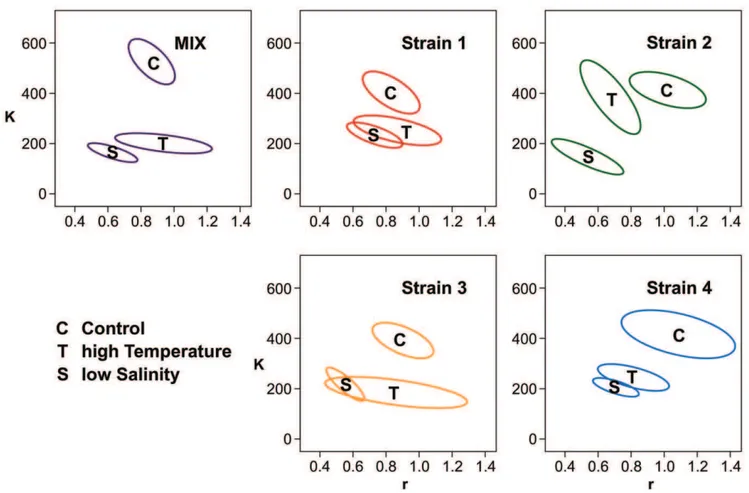
On average, the S. marinoi cultures reached maximum cell densities and growth rates of roughly 1.86105 cells ml–1 and 0.9460.1 divisions d–1in the control treatment, 16105cells ml–1 and 0.8360.1 divisions d–1in the high temperature treatment and 0.66105cells ml–1and 0.6360.09 divisions d–1in the low salinity treatment. Figure 2 & 3 present the growth characteristics of all strains, represented by the respective confidence interval of the bootstrappedr-Kvalues. In both stressed treatments, all strains and
Figure 1. Growth curves.Growth curves of strain 1–4 (red, green, yellow and blue, respectively) and the mixture (violet) comprising all four clones in equal proportions. Each panel represents one salinity6temperature treatment (Control: Salinity 25, Temperature 20uC; high T: Salinity 25, Temperature 28uC; low S: Salinity 7, Temperature 20uC; high T/low S: Salinity 7, Temperature 28uC). Data points represent the mean of the four replicates; error bars represent standard error of mean. Start concentrations were 6000 cells ml–1in all treatments. Biomass units are raw fluorescence data. The experiment was terminated on day 9.
the mixture showed different growth dynamics than in the control treatment (Figure 2). Interestingly, both dimensions (randK) were needed to separate the growth curves in all treatments, highlight-ing the importance of assesshighlight-ing both parameters jointly. When we compared the growth curves of the strains within treatments, we observed no differences between strains in the control group, and only between strain 2 and strain 3 in the high temperature treatment. In the low salinity treatment, the growth curve of strain 2 differed from strain 1 and 4, and strain 3 differed from strain 1. When we compared the growth curves of each strain between the three treatments (Figure 3) we found differences between the low salinity and the high temperature treatment for strain 2, but not for strain 1, 3 and 4. These observations suggested that the strains did not grow differentlyper se, but that they reacted differently to the two stressors.
Comparisons of the Mixture and Monocultures
The mixture did not consistently differ from the monocultures. In the control, the mixture showed higher growth than strain 1, and in the high temperature treatment it showed lower growth than strain 2. In the low salinity treatment the growth curves of the mixture showed lower growth than strain 1 and strain 4 (Figure 2). We assessed the relative abundance of the strains in the early stationary growth phase in the control and the low salinity treatment. Strain 4 dominated the mixture in both treatments with average relative abundances of over 80% (Figure 4). This dominance was consistent throughout all the replicates, with a minimum abundance of 78%. We observed no differences between the abundances of strain 1, 2 and 3 (one factor ANOVA with ‘‘strain’’ as factor and a subsequent post-hoc Tukey HSD test, P.0.15 in all cases).
Stress and Biodiversity Calculations
It was not possible to assess synergistic effects of the combined stress treatment as the 95% confidence intervals of the expected distributions included or were below 0 in all cases. Although this overlap was primarily observed for theK-axis,Kandrcannot be considered independent variables, and an independent interpre-tation of r would be invalid. Despite this, we were able to determine that the combined effect of both stressors was additive at a minimum.
The calculation of the biodiversity effects (Figure 5) showed
a net positive biodiversity effect (119676; [mean 695%
confidence interval]), a positive complementarity effect
(1146103), but no selection effect (5663) in the control treatment. In contrast, the calculation in the low salinity treatment showed a negative net biodiversity effect (–38639, significant at the 94% confidence interval) and complementarity effect (–39638), but again no selection effect (1.6619) was observed. In the high temperature treatment, the net bio-diversity effect was negative (–65648) but complementarity and selection effects could not be assessed.
Discussion
Our results showed that 1) the different genotypes were phenotypically different, 2) strong competition between the genotypes occurred, including competition mechanisms beyond outgrowing as one strain with average monoculture performance dominated the mixture, and 3) that the effects of genotypic diversity were different under control and stress conditions, but that these effects were not easily predictable from observations of the monocultures. Below, we discuss the results in more detail.
In concordance with hypothesis 1, the overall growth was reduced in the low salinity and high temperature treatments. The combined effect of both stressors was lethal (Figure 1). Based on the strong reaction caused by each single stressor, this was predicted based on an additive stress model (i.e.the sum of the impacts was expected to push biomass below 0). Additive interactions are proposed for stressors that act on indepent physiological processes which was likely the case in our experiment [38]. The physiological explanation for the 100% mortality was hence most likely the metabolic cost of each stress resistance mechanism, which exceeded the threshold of viability when both stressors were combined. This could include the activity of ion pumps to adjust the osmotic pressure under salinity stress, or the expression of heat-shock-proteins as a reaction to temperature stress. Due to the strength of each single stressor, we were unable to assess synergism (i.e.a greater than additive effect).
Contrary to hypothesis 2a, we found no differences in growth dynamics among the strains within the control treatment. We did, however, observe differences between strains within the high temperature and the low salinity treatment as well as in the response of at least one strain (strain 2) between the high temperature and the low salinity treatments, thereby fulfilling hypothesis 2b.
According to hypothesis 3, the most productive strain in monoculture should out-compete the other strains in the mixture and therefore become numerically dominant over time (i.e.positive selection effect [20]). The treatment in which we observed the greatest differences between strains in monocultures was the low salinity treatment. Strains 1 and 4 performed better than strain 2 with the highest average performance reached by strain 1 (Figure 2). The dominant strain in the mixture at the end of the
experiment was strain 4 (.80%). In contrast to what was
expected, the mixture performed worse than both strains 1 and 4, and we observed a negative net biodiversity effect. Strain 4 was equally dominant in the control treatment, although no differences in performance of the single strains were observed in monoculture. Moreover, in this treatment we observed a positive net biodiversity effect. Hence, even though one strain dominated in mixture, the dominant strain could not be predicted by the performances of the different strains in monoculture.
partitioning) and negative complementarity (e.g. competition) acted simultaneously, with an increasing relative importance of negative complementarity in stressful environments. This would assume mechanisms of direct competition between the four strains, which is plausible but has not been described to date. At the species level, however, similar results were found in an experiment with different Chladomydomonas species [16], where non-trans-gressive over-yielding was observed in some nutrient-environments
but not in others. It was concluded that strong but different types of interactions took place.
It has been argued that negative complementarity can be the outcome of competition among functionally similar organisms [47]. Indeed, Cadotte et al. [48] found that phylogenetic distance is the single best predictor for plant productivity in mixtures, and Jousset et al. [49] reported that genotypic richness reduces the growth rate of a bacterial community, whereas growth is enhanced by genotypic dissimilarity between community members. Likewise,
Figure 2. Growth dynamics.Growth dynamics of the four strains in monocultures (red, green, yellow and blue for strain 1–4 respectively) and the mixture (violet) in the three treatments in which growth was observed, plotted per treatment. Control: Temperature = 20uC, Salinity = 25; high T: Temperature = 28uC, Salinity = 27; low S: Temperature = 20uC, Salinity = 7. The ellipses represent 95% confidence intervals of the bootstrapped parameter distributions of the modelled growth curves.Krepresents maximum biomass and the units are raw fluorescence of Chla,andris the maximum growth rate given in cell divisions per day. The range of the axes is standardized in order to represent the same amount of relative variance around the overall mean ofrandK, respectively.
Figure 3. Growth dynamics.Growth dynamics of the four strains in monocultures (red, green, yellow and blue for clone 1–4 respectively) and mixture (violet) in the three treatments in which growth was observed, plotted per strain and the mixture. [C]: Temperature = 20uC, Salinity = 25; [T] = 28uC, Salinity = 27; [S]: Temperature = 20uC, Salinity = 7. The ellipses represent 95% confidence intervals of the bootstrapped parameter distributions of the modelled growth curves.Krepresents maximum biomass and the units are raw fluorescence of Chla, andris maximum growth rate given in cell divisions per day. The range of the axes is standardized in order to represent the same amount of relative variance around the overall mean ofrandK, respectively.
doi:10.1371/journal.pone.0045007.g003
Figure 4. Relative abundances of the strains.Relative abundances of the strains 1–4 (red, green, yellow and blue, respectively) in the mixture of the control (Salinity 25, Temperature 20uC) and the low salinity (Salinity 7, Temperature 20uC) treatments. Proportions are given in percentages and represent the average abundance of the four replicates. Error bars are standard error of the mean.
in Bell’s experiment [17], mixtures composed of half-siblings outperformed mixtures composed of full-siblings. Our experiment was composed of four randomly chosen strains and we have no information on the relatedness of these strains. Although high similarity is consistent with the lack of differences between the strains under control conditions, it does not explain the positive complementarity observed in this treatment. Furthermore, phe-notypical dissimilarity was higher in the high temperature and the low salinity treatment where negative complementarity was observed. In summary, we found that diversity effects occurred, but we can only speculate about the underlying mechanisms.
One of the most intriguing outcomes was the dominance of strain 4, which out-competed all other strains in the two treatments for which we had information on the final clonal composition. In a community under exponential growth with equal initial concentrations and incubation time, the only explanation for one strain becoming dominant over time is a higher growth rate. Although the growth rates of the four strains did not differ in monocultures, the relative growth rates of the individual strains in the mixture must have been different while simultaneously sustaining the overall community growth rate. Different growth rates in the mixture indicate the existence of a mechanism that affects growth rates only when strains coexist, thereby excluding classical explanations such as differences in the efficiency of resource use [50] that should equally enhance growth rates in the monocultures. Sedimentation rates were high in our experimental system and the diatoms spent most of the time at the bottom of the flasks. One possible explanation for the dominance of strain 4 in the mixture could be better access to light through a slower rate of sedimentation. In fact, strain 4 had a slightly longer average chain length than strains 1–3 (one factor ANOVA with ‘‘strain’’ as factor and subsequent post-hoc Tukey HSD test, P,0.1 in all cases). It is unclear, however, if longer chain length increases floatability in living cells [51], and stratification in only 4 cm water column seems unrealistic. A positive correlation between chain length and growth rate has also been reported [52], meaning that longer chains could actually be the effect of – and not the reason for – a competitive advantage. Another possible
explanation could be chemical interference (allelopathy), which can inhibit the growth of competitors. Diatoms are known to produce toxic polyunsaturated aldehydes (PUAs) in response to cell damage [53]. Taylor et al. [54] described different production potentials of PUAs for genetically distinct strains ofS. marinoi,and the release of PUAs without cell damage was also reported [55], yet the latter occurred only in late stationary growth phase. Although allelopathy is a well-documented phenomenon in autotrophic plankton [56], it has not been thoroughly studied at intra-specific level and an explanation for this is less clear. The compounds produced need to be extremely strain-specific, or one would need to assume a trade-off between an enhanced pro-duction of and a decreased vulnerability to the produced compounds for a specific strain. It is not clear to what extentS. marinoiis vulnerable to its own compounds.
In times of rapid global change, it is necessary to assess the role of genetic diversity in coping with multiple drivers of environ-mental shift. While the combination of stressors was lethal, we found that some algal strains grew better than others in low salinity. Only by simultaneously manipulating several stressors as well as genetic diversity can we increase our understanding of the potential importance of intraspecific biodiversity for ecosystem processes such as productivity. While we observed strong competition among strains, the mechanism behind the superiority of the dominant strain is difficult to assess. Further studies are required to evaluate the processes involved in intraspecific competition in microalgae. The study confirms, however, that many processes observed at the species level are relevant at the level of genotypes, and that genetic diversity may therefore play a comparably important role in natural systems and in changing environmental conditions.
Supporting Information
Figure S1 Alternative presentation of the results in Figure 1.Growth curves of strain 1–4 (red, green, yellow and blue, respectively) and the mixture (violet). The five panels represent the four strains and the mixture and the lines represent
the growth curves of the respective strain in the four treatments. Data points represent the mean of the four replicates; error bars represent standard error of mean. Biomass units are raw fluorescence data.
(TIF)
Acknowledgments
We thank David Nerini for suggesting the method for growth-curve comparisons and for help with the [R]-code. We also acknowledge Per Jonsson and David Kleinhans for help with the statistical analysis, Jenny Egardt for help in the laboratory, Annika O’Dea for language editing and
the editor and one anonymous reviewer for constructive comments that improved the manuscript. The fragment analysis was performed at the Genomics Core Facility, Sahlgrenska Academy, University of Gothenburg, by Dr Elham Rekabdar. This work was partly performed within the Linnaeus Centre for Marine Evolutionary Biology (http://www.cemeb. science.gu.se/).
Author Contributions
Conceived and designed the experiments: FR AG LG. Performed the experiments: FR. Analyzed the data: FR. Contributed reagents/materials/ analysis tools: FR AG LG. Wrote the paper: FR AG LG.
References
1. Naeem S, Bunker DE, Hector A, Loreau M, Perrings C (2009) Biodiversity, ecosystem functioning, and human wellbeing: an ecological and economic perspective. Oxford: Oxford University Press.
2. Cardinale BJ, Matulich K, Hooper DU, Byrnes JE, Duffy E, et al. (2011) The functional role of producer diversity in ecosystems. American Journal of Botany 98: 572–592. doi: 10.3732/ajb.1000364.
3. Hooper DU, Adair EC, Cardinale BJ, Byrnes JEK, Hungate BA, et al. (2012) A global synthesis reveals biodiversity loss as a major driver of ecosystem change. Nature. doi: 10.1038/nature11118.
4. Griffin JN, O’Gorman EJ, Emmerson MC, Jenkins SR, Klein A-M, et al. (2009) Biodiversity and the stability of ecosystem functioning. In: Naeem S, Bunker DE, Hector A, Loreau M, Perrings C, editors. Biodiversity, ecosystem functioning, and human wellbeing: an ecological and economic perspective. Oxford: Oxford University Press. 78–93.
5. Frankham R (2005) Genetics and extinction. Biological Conservation 126: 131– 140. doi: 10.1016/J.Biocon.2005.05.002.
6. Smithson JB, Lenne JM (1996) Varietal mixtures: a viable strategy for sustainable productivity in subsistence agriculture. Annals of Applied Biology 128: 127–158. doi: 10.1111/j.1744-7348.1996.tb07096.x.
7. Zhu Y, Chen H, Fan J, Wang Y, Li Y, et al. (2000) Genetic diversity and disease control in rice. Nature 406: 718–722. doi: 10.1038/35021046.
8. Hughes AR, Inouye BD, Johnson MTJ, Underwood N, Vellend M (2008) Ecological consequences of genetic diversity. Ecology Letters 11: 609–623. doi: 10.1111/j.1461-0248.2008.01179.x.
9. Whitham TG, Bailey JK, Schweitzer JA, Shuster SM, Bangert RK, et al. (2006) A framework for community and ecosystem genetics: from genes to ecosystems. Nature Reviews Genetics 7: 510–523. doi: 10.1038/nrg1877.
10. Reusch TBH, Ehlers A, Ha¨mmerli A, Worm B (2005) Ecosystem recovery after climatic extremes enhanced by genotypic diversity. Proceedings of the National Academy of Sciences of the United States of America 102: 2826–2831. doi: 10.1073/pnas.0500008102.
11. Ehlers A, Worm B, Reusch TBH (2008) Importance of genetic diversity in eelgrass Zostera marinafor its resilience to global warming. Marine Ecology Progress Series 355: 1–7. doi: 10.3354/meps07369.
12. Gamfeldt L, Walle´n J, Jonsson PR, Berntsson KM, Havenhand JN (2005) Increasing intraspecific diversity enhances settling success in a marine in-vertebrate. Ecology 86: 3219–3224. doi: 10.1890/05-0377.
13. Hughes AR, Stachowicz JJ (2004) Genetic diversity enhances the resistance of a seagrass ecosystem to disturbance. Proceedings of the National Academy of Sciences of the United States of America 101: 8998–9002. doi: 10.1073/ pnas.0402642101.
14. Schweitzer JA, Bailey JK, Hart SC, Whitham TG (2005) Nonadditive effects of mixing cottonwood genotypes on litter decomposition and nutrient dynamics. Ecology 86: 2834–2840. doi: 10.1890/04-1955.
15. Johnson MTJ, Lajeunesse MJ, Agrawal AA (2006) Additive and interactive effects of plant genotypic diversity on arthropod communities and plant fitness. Ecology Letters 9: 24–34. doi: 10.1111/j.1461-0248.2005.00833.x.
16. Bell G (1990) The ecology and genetics of fitness in chlamydomonas.2. the properties of mixtures of strains. Proceedings of the Royal Society of London Series B-Biological Sciences 240: 323–350.
17. Bell G (1991) The ecology and genetics of fitness in chlamydomonas.4. the properties of mixtures of genotypes of the same species. Evolution 45: 1036– 1046.
18. Aguirre JD, Marshall DJ (2012) Genetic diversity increases population productivity in a sessile marine invertebrate. Ecology 93: 1134–1142. doi: 10.1890/11-1448.1.
19. Drummond EBM, Vellend M (2012) Genotypic diversity effects on the performance of Taraxacum officinale populations increase with time and environmental favorability. Plos One 7: e30314. doi: 10.1371/journal.-pone.0030314.
20. Loreau M, Hector A (2001) Partitioning selection and complementarity in biodiversity experiments. Nature 412: 72–76. doi: 10.1038/35083573. 21. Trenbath B (1974) Biomass productivity of mixtures. Advances in Agronomy 26:
177–210.
22. Norberg J, Swaney DP, Dushoff J, Lin J, Casagrandi R, et al. (2001) Phenotypic diversity and ecosystem functioning in changing environments: a theoretical
framework. Proceedings of the National Academy of Sciences of the United States of America 98: 11376–11381. doi: 10.1073/pnas.171315998. 23. Sarno D, Kooistra WHCF, Medlin LK, Percopo I, Zingone A (2005) Diversity
in the genusSkeletonema(Bacillariophyceae). ii. An assessment of the taxonomy of S. costatum like species with the description of four new species. Journal of Phycology 41: 151–176. doi: 10.1111/j.1529-8817.2005.04067.x.
24. Kooistra WHCF, Sarno D, Balzano S, Gu H, Andersen RA, et al. (2008) Global diversity and biogeography ofSkeletonemaspecies (Bacillariophyta). Protist 159: 177–193. Doi: 10.1016/j.protis.2007.09.004.
25. Godhe A, McQuoid MR, Karunasagar I, Rehnstam Holm AS (2006) Comparison of three common molecular tools for distinguishing among geographically separated clones of the diatomSkeletonema marinoi Sarno et Zingone (Bacillariophyceae) Journal of Phycology 42: 280–291. doi: 10.1111/ j.1529-8817.2006.00197.x.
26. Godhe A, Ha¨rnstro¨m K (2010) Linking the planktonic and benthic habitat: genetic structure of the marine diatomSkeletonema marinoi. Molecular Ecology 19: 4478–4490. doi: 10.1111/j.1365-294X.2010.04841.x.
27. Saravanan V, Godhe A (2010) Genetic heterogeneity and physiological variation among seasonally separated clones ofSkeletonema marinoi(Bacillariophyceae) in the Gullmar Fjord, Sweden. European Journal of Phycology 45: 177–190. doi: 10.1080/09670260903445146.
28. Grime JP (1989) The stress debate - symptom of impending synthesis. Biological Journal of the Linnean Society 37: 3–17.
29. Claquin P, Probert I, Lefebvre S, Veron B (2008) Effects of temperature on photosynthetic parameters and TEP production in eight species of marine microalgae. Aquatic Microbial Ecology 51: 1–11. doi: 10.3354/ame01187. 30. Balzano S, Sarno D, Kooistra WHCF (2011) Effects of salinity on the growth
rate and morphology of tenSkeletonemastrains. Journal of Plankton Research 33: 937–945. doi: 10.1093/plankt/fbq150.
31. Ha¨rnstro¨m K, Ellegaard M, Andersen TJ, Godhe A (2011) Hundred years of genetic structure in a sediment revived diatom population. Proceedings of the National Academy of Sciences of the United States of America 108: 4252–4257. doi: 10.1073/pnas.1013528108.
32. Guillard RRL (1975) Culture of phytoplankton for feeding marine invertebrates. New York: Plenum Press. 26–60.
33. Phinney DA, Yentsch CS (1985) A novel phytoplankton chlorophyll technique: toward automated analysis. Journal of Plankton Research 7: 633–642. doi: 10.1093/plankt/7.5.633.
34. Kremp A, Godhe A, Egardt J, Dupont S, Suikkanen S, et al. (2012) Intraspecific variability in the response of bloom forming marine microalgae to changing climatic conditions. Ecology and Evoloution 2(6): 1195–1207.
35. Kooistra WHCF, De Stefano M, Mann DG, Salma N, Medlin LK (2003) Phylogenetic position ofToxarium, a pennate like lineage within centric diatoms (Bacilliarophyceae). Journal of Phycology 39: 185–197. doi: 10.1046/j.1529-8817.2003.02083.x.
36. Almany GR, DE Arruda MP, Arthofer W, Atallah ZK, Beissinger SR, et al. (2009) Permanent genetic resources added to molecular ecology resources database 1 May 2009-31 July 2009. Molecular Ecology Resources 9: 1460–1466. doi: 10.1111/j.1755-0998.2009.02759.x.
37. R Development Core Team (2011) R: a language and environment for statistical computing. R Foundation for Statistical Computing. Available: http://www.r-project.org/. Accessed 2012 Aug 26.
38. Folt CL, Chen CY, Moore MV, Burnaford J (1999) Synergism and antagonism among multiple stressors. Limnology and Oceanography 44: 864–877. 39. Genz A, Bretz F, Miwa T, Mi X, Leisch F, et al. (2011) mvtnorm: multivariate
normal and t distributions. R package version 0.9-9991.
40. Wickham H (2011) The split-apply-combine strategy for data analysis. Journal of Statistical Software 40: 1–29.
41. Wickham H (2009) ggplot2: elegant graphics for data analysis. New York: Springer.
42. Parker JD, Salminen JP, Agrawal AA (2010) Herbivory enhances positive effects of plant genotypic diversity. Ecology Letters 13: 553–563. doi: 10.1111/j.1461-0248.2010.01452.x.
44. Cook-Patton SC, McArt SH, Parachnowitsch AL, Thaler JS, Agrawal AA (2010) A direct comparison of the consequences of plant genotypic and species diversity on communities and ecosystem function. Ecology 92: 915–923. doi: 10.1890/10-0999.1.
45. Rauch G, Kalbe M, Reusch TBH (2008) Partitioning average competition and extreme-genotype effects in genetically diverse infections. Oikos 117: 399–405. doi: 10.1111/j.2007.0030-1299.16301.x.
46. Hughes AR, Best RJ, Stachowicz JJ (2010) Genotypic diversity and grazer identity interactively influence seagrass and grazer biomass. Marine Ecology Progress Series 403: 43–51. doi: 10.3354/meps08506.
47. Hillebrand H, Matthiessen B (2009) Biodiversity in a complex world: consolidation and progress in functional biodiversity research. Ecology Letters 12: 1405–1419. doi: 10.1111/j.1461-0248.2009.01388.x.
48. Cadotte MW, Cardinale BJ, Oakley TH (2008) Evolutionary history and the effect of biodiversity on plant productivity. Proceedings of the National Academy of Sciences of the United States of America 105: 17012–17017. doi: 10.1073/ pnas.0805962105.
49. Jousset A, Schmid B, Scheu S, Eisenhauer N (2011) Genotypic richness and dissimilarity opposingly affect ecosystem functioning. Ecology Letters 14: 537– 545. doi: 10.1111/j.1461-0248.2011.01613.x.
50. Titman D (1976) Ecological competition between algae: experimental confirmation of resource-based competition theory. Science 192: 463–464. doi: 10.1126/science.192.4238.463.
51. Waite A, Fisher A, Thompson PA, Harrison PJ (1997) Sinking rate versus cell volume relationships illuminate sinking rate control mechanisms in marine diatoms. Marine Ecology Progress Series 157: 97–108. doi: 10.3354/ meps157097.
52. Takabayashi M, Lew K, Johnson A, Marchi A, Dugdale R, et al. (2006) The effect of nutrient availability and temperature on chain length of the diatom, Skeletonema costatum. Journal of Plankton Research 28: 831–840. doi: 10.1093/ plankt/fbl018.
53. Lauritano C, Borra M, Carotenuto Y, Biffali E, Miralto A, et al. (2011) Molecular evidence of the toxic effects of diatom diets on gene expression patterns in copepods. Plos One 6: e26850. doi: 10.1371/journal.pone.0026850. 54. Taylor RL, Abrahamsson K, Godhe A, Wangberg SA (2009) Seasonal Variability in polyunsaturated aldehyde production potential among strains of Skeletonema marinoi (Bacillariophyceae). Journal of Phycology 45: 46–53. doi: 10.1111/j.1529-8817.2008.00625.x.
55. Vidoudez C, Pohnert G (2008) Growth phase-specific release of polyunsaturated aldehydes by the diatomSkeletonema marinoi. Journal of Plankton Research 30: 1305–1313. doi: 10.1093/plankt/fbn085.