BFC METHOD FOR PREDICTION OF TRANSIENT HEAD
ON SEEPAGE PATH
Sherly Hartono
Civil Engineering Department, Faculty of Science and Technology, Bina Nusantara University Jln K.H. Syahdan No. 9, Palmerah, Jakarta Barat 11480
ABSTRACT
Seepage causes weakening of levees and can cause levee failure or overtopping due to levee settlement. A numerical method, called the boundary fitted coordinate (BFC) method, was developed to determine seepage through a levee and the transient head on the seepage path due to the changing water level during a flood. The BFC transforms the physical coordinate system into a computational curvilinear coordinate system. The grid generated in this method accurately represents the boundary of the system regardless of its complexity.
Keywords: BFC method, critical head, flood, free surface, levee, piping, seepage.
ABSTRAK
Rembesan mengakibatkan kerapuhan sebuah tanggul dan bisa menyebabkan tanggul gagal atau melebihi batas kemampuan tanggul. Dalam metode numerik, disebut BFC atau boundary fitted coordinate, yang dikembangkan untuk menentukan rempegan melalui tanggul dan atasan tambahan dalam rembesan untuk mengubah tingkatan air selama banjir. BFC mentransformasi sistem koordinasi fisik melalui sistem koordinat komputasi kurvilinear. Kisi yang digunakan dalam metode ini merepresentasikan batasan kompleks sistem secara akurat.
INTRODUCTION
Seepage flows may cause piping and the weakening of a levee. As a result, seepage must be controlled to avoid levee failure. Analysis of seepage is needed to predict the seepage path and rate, develop measures to reduce the magnitude of seepage flow, evaluate excessive soil saturation, determine seepage force and uplift pressure that may lead to levy failure, evaluate proposed levee design and maintenance alternatives, reduce the risk of levee failure, determine the likelihood of damage to the levee due to piping, and evaluate measures to control piping. During floods, the water level on the riverside of a levee can change dramatically. As river stage rises or falls, the location of the free surface where it intersects the upstream levee face changes. This movement of the free surface stores or yields far more water than the quantity of water stored or released due to the compressibility effects. Therefore, it is reasonable to assume that flow through the levee during flood will be unsteady. The unsteadiness of the flow is caused by the moving free surface.
When seepage paths are disturbed, the transition from the original flow line configuration to the new flow line configuration can take a significant time. Changes in the position of the free water surface are not instantaneous because of specific yields of the soil material combined with slow seepage of water through the levee. In modeling transient free surface, not only boundary conditions must be known but also the initial condition at the start of the event. During a flood the free surface boundary moves in time, subject to certain conditions. Consequently, the movement of the free surface tends to dominate the flow pattern within the levee. In certain instances, critical conditions can occur during this change and it is, therefore, important to investigate the time variant seepage behavior. When head no longer changes with time, a steady state is reached. Some approximate numerical solutions using finite difference methods and finite element methods have been developed to determine the location of the head by discrediting the problem domain and solving the governing equations in this domain. These methods often experience instability and smoothing problems. In addition, it is difficult to accurately represent the problem domain because of its complicated shape, except when the finite element method is employed. The objective of this study is therefore to develop an improved yet simple method of solution using the boundary fitted coordinate method for determining transient head during seepage.
METHODS
Although there are many analytical and numerical solutions developed for steady state seepage, there is still a need for evaluation of the seepage path in transient conditions. This analysis is important, since critical conditions can occur before the steady state condition has been reached. In general, any specification of boundary conditions for the second order parabolic partial differential equations applicable to unsteady state seepage flow should include the geometric shape of the boundary, a statement of how the dependent variable varies on the boundary, and the initial condition.
transient problems and the smoothness of the solution can be obtained using the Laplace equation system generation.
Transient Seepage Through an Earth Dam
The general governing equation for unsteady seepage through an anisotropic and heterogeneous earth dam can be expressed as:
t
h
S
y
h
k
x
h
k
y
y
h
k
x
h
k
x
xx xy yx yy∂
∂
=
⎟⎟
⎠
⎞
⎜⎜
⎝
⎛
∂
∂
+
∂
∂
∂
∂
+
⎟⎟
⎠
⎞
⎜⎜
⎝
⎛
∂
∂
+
∂
∂
∂
∂
(1)where h = head; kxx, kxy, kyx, kyy = hydraulic conductivity components in the x, y, and z directions; S = specific storage coefficient; t = time.
For simplicity, the earth dam is considered to be isotropic and homogeneous. Equation (1), therefore, becomes:
t
h
S
y
h
x
h
k
∂
∂
=
⎟
⎟
⎠
⎞
⎜
⎜
⎝
⎛
∂
∂
+
∂
∂
2 2 2 2 (2)where k = permeability coefficient.
For solution of equation (2), initial and boundary conditions need to be specified. These conditions must be specified on all sides of the solution domain and to correctly represent the free surface. The boundary conditions can be described as follows:
H
h(x,y,t)= on free surface (F) (3)
0
ˆ
=
∇
h(x,y,t).
n
on free surface (F) (4) H,y,t)
h(x=0 = on left side (L) (5)
tail
H
w,y,t)
h(x
=
=
on right side (R) (6)H
h(x,y,t)= on seepage face (S) (7)
0
ˆ
=
∇
h(x,y,t).
n
on bottom side (B) (8)Equations (3) to (8) can be succinctly expressed as H
) w,y,t
h(x= <0 = (9)
tail
H
)
w,y,t
h(x
=
=
0
=
(10)Equations (1) to (10) define the problem of seepage through the earth dam.
Boundary Fitted Coordinate Method of Solution
generator, more specifically the Laplace grid generator. In order to make use of a general boundary-conforming curvilinear coordinate system in the solution of partial differential equations, the governing and boundary equations must also be transformed to the curvilinear coordinates, where the independent variables are time and Cartesian coordinates. When a coordinate system has been generated, the value of the Cartesian coordinates will be available as functions of the curvilinear coordinates. Each step and the corresponding equations of this method are explained in what follows.
Grid Generation
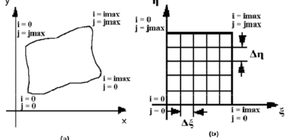
The boundary fitted coordinate (BFC) method has the ability to conform to the boundaries of the system regardless of its shape. This feature increases the accuracy of the solution to be obtained. The most important characteristic of this method is that the transformation is performed so that the physical Cartesian coordinates (x, y) become dependent variables and the curvilinear coordinates (ξ, η)
become independent variables. A generated grid is then defined as a set of points formed by the intersections of the lines of a boundary conforming to the curvilinear coordinate system. The principal feature of this system is that some coordinate line is coincident with each section of the boundary in the physical region.
The use of coordinate line intersections for defining the grid points provides a means that allows all computations to be done on a fixed square grid after the governing partial differential equations are transformed as shown in Figure 1. The size of the intervals then determines the number of grid lines generated for a particular problem. Computations may be simplified by first transforming the governing equations so that the physical Cartesian coordinates become dependent variables and the curvilinear coordinate’s independent variables. The boundary value problem in the transformed domain then involves generating the values of the physical Cartesian coordinates, x(ξ, η) and y(ξ, η)
in the transformed domain from the specified boundary values of x(ξ,η) and y(ξ,η) on the rectangular boundary of the transformeddomain, the boundary being formed of segments of constant ξ or η. There is a unique correspondence between Cartesian and curvilinear coordinate systems. The mapping of the physical region onto the transformed region must be one to one, so that every point in the physical domain corresponds to one and only one point in the transformed domain and vice versa.
Figure 1. Transformation of problem domain from the (a) physical Cartesian coordinate system to (b) computational curvilinear coordinate system
For conversion between the Cartesian and curvilinear coordinate systems, the following transformation relationships are used (Thompson, 1977):
J y
J x
ξy =− η (12)
J
y
η
x=
−
ξ (13)J
x
η
y=
ξ (14)Where
ξ η η ξ
y
x
y
x
J
=
−
(15)In order to make use of a general boundary-conforming curvilinear coordinate system in the solution of partial differential equations, the equations must also be transformed to the curvilinear coordinates, where the independent variables are time and Cartesian coordinates. The resulting equations are of the same type as the original ones, but are more complicated because they contain more terms and variable coefficients. The domain, on the other hand, is greatly simplified since it is transformed to a fixed rectangular region regardless of its shape and movement in the physical space.
As mentioned before, there is a need for a smoothing procedure to avoid instability. In the BFC method, this smoothing is done by using the elliptic grid generator, more specifically the Laplace grid generator which is known to have smoothing properties and thus the grids generated from this equation are the smoothest grid possible. Since smoothing procedure is already incorporated into the BFC method, finite differences can then be applied to solve the problem without experiencing the instability that can occur when they are applied to the problem described in the Cartesian coordinates.
In order to accurately describe the domain, at least four corner points must be chosen to represent the start and end of the boundaries in each direction. The rest of the boundaries can then be obtained from the equation which describes the boundary. After determination of boundary points, a grid generator is used to calculate the interior nodes of the solution domain. Two kinds of grid generator are used in generating a solution, which are the algebraic grid generator and the partial differential grid generator.
Algebraic Grid Generator
For initial grid generation, interior nodes of the solution domain area can be generated from direct interpolation from the boundaries using algebraic grid generation system, such as a unidirectional interpolation or a multi-directional interpolation.
Partial Differential Equation Grid Generator
As mentioned before, in order to guarantee the smoothness of the solution, the Laplace equation is used to generate a grid system that will be used in solving the governing equations. Following Thompson (1977), Thompson and Warsi (1982), Thompson et al. (1985), the following formulas are used, where ξ and η are the transformed curvilinear coordinates.
0
=
+
yy xxξ
ξ
(16)0
=
+
yy xxη
η
(17)Following the procedure described by Thompson (1977) and using equations (11)-(14), equations (16) and (17) can be rearranged to yield the following formula:
0
2
+
=
−
ξη ηηξξ
x
x
α
x
(18)0
2
+
=
−
ξη ηηξξ
y
y
α
y
(19)where 2 2 η η
y
x
α
=
+
(20)η ξ η ξ
x
y
y
x
+
=
(21)2 2
η ξ x x +
= (22)
Transformation of the governing equation is then done to ensure compatibility with the computational domain. The transformed form of equation (2) assuming homogeneous and isotropic conditions in the transformed domain is:
t h S h h
αhξξ ξη ηη
∂ ∂ = +
−2 (23)
Transformation from the Cartesian coordinate system (x, y) to the curvilinear coordinate system (ξ, η) is not only done on the governing equation, but it is also done on the initial condition and boundary conditions which describe the problem. This is done so that there is consistency in the coordinate system used in solving the problem. After the problem is solved, the corresponding result is then transformed back into the original coordinate system, which is the Cartesian coordinate system (x, y).
The boundary conditions are also transformed into curvilinear coordinates so that they will be compatible with the governing equations
(
ξ
,
η
,t
)
H
h
=
on free surface (F) (24)0
=
− ξ
η h
h on free surface (F) (25)
H t) ,η
h(ξ =0 , = on left side (L) (26)
(
ξ
w,
η
t
)
H
tailh
=
,
=
on right side (R) (27)(
ξ
,
η
,t
)
H
h
=
on seepage face (S) (28)0
=
− ξ
η h
h on bottom side (B) (29)
2 1
)
(Δ 2 ≤
Δ x
t D
(30)
Applying these conditions to the curvilinear coordinate system yield the following equations
( )
[
]
kF SJ
t
2 )
( 2 2
2 Δ
ξ
+ Δη
≤
Δ (31)
where F is the maximum value between α, 2β, or γ.
The formula for calculation of the new head position after each time step is described, assuming the porous medium to be isotropic and homogeneous, is:
⎥
⎦
⎤
⎢
⎣
⎡
⎟⎟
⎠
⎞
⎜⎜
⎝
⎛
∂
∂
−
−
∂
∂
Δ
−
=
a
y
h
y
h
w
S
t
k
Δ
H
y2
tan
1
(32)where tan a = the head difference between two nodes adjacent to the nodes being calculated at the moment divided by the length between the two nodes, and Sy = specific yield. Equation (32) is then transformed into the curvilinear coordinate system
Transient Seepage through a Levee
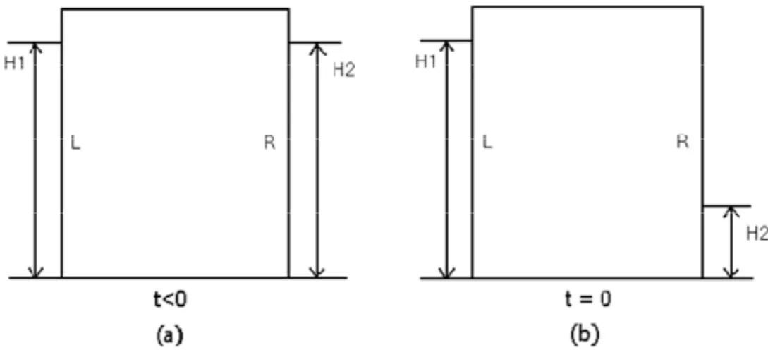
The model developed previously was applied to a levee to show the versatility of the model in handling different kinds of domains. A levee with different slopes on the riverside and the landside is used as the domain of this problem. The slope on the landside of the levee is steeper than the slope on the riverside of the levee. The height of the levee is 8 m and the width of the crest is 20 m. After transformation of equations as described previously, the domain becomes rectangular in the computational coordinate system. A cross section of the levee in the physical domain and the computational domain is shown in Figure 2. To simulate unsteady state condition, the water level on the riverside of the levee is suddenly dropped to a 2 m elevation at time t = 0 from its previous position at 5 m. The water elevation is kept at 2 m until the solution reaches a steady state. There is no tailwater on the landside of the levee.
Using the same techniques described in the previous example, the transformed governing equation and boundary conditions are:
0
2 + =
+ ξη ηη
ξξ h h
αh (33)
(
ξ
,
η
,t
)
H
h
=
on free surface (F) (34)0
=
− ξ
η h
h on free surface (F) (35)
2 ,
0 =
= ,ηt)
h(ξ on left side (L) (36)
(
ξ
=
w,
η
,
t
)
=
0
h
on right side (R) (37)(
ξ
,
η
,t
)
H
h
=
on seepage face (S) (38)0
=
− ξ
η h
h on bottom side (B) (39)
The time steps calculation can be obtained by using the minimum value obtained from these equations
( )
[
]
kF SJ t 2 )( 2 2
2 Δ
ξ
+ Δη
≤
Δ (40)
Using the method described previously, the formula for calculation of the new head position after each time step is described by the following equation
⎥
⎥
⎦
⎤
⎢
⎢
⎣
⎡
⎟
⎟
⎠
⎞
⎜
⎜
⎝
⎛
−
−
−
⎟
⎟
⎠
⎞
⎜
⎜
⎝
⎛
−
Δ
−
=
a
J
h
h
J
h
h
w
S
t
k
Δ
H
η ξ η ξy
2
tan
1
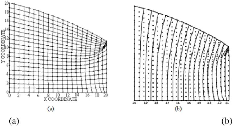
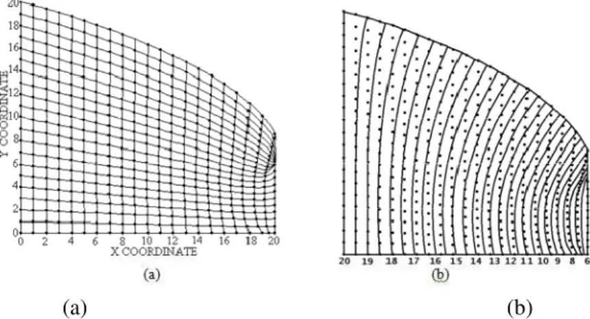
(41)After initial coordinates of the new free surface are calculated, the boundary conditions are calculated again until steady state is achieved. For this problem, the values k = 0.12 m/d and Sy = 0.15 are used. Figures 3 and 4 show the grid generation and the head distribution for different time steps. For each time step, the solutions shown are solutions at steady state, where the height and hydraulic head no longer change with each iteration. The elevation of the seepage face from the start of the simulation decreases until it reaches the end of simulation. This is to be expected as the ratio of the width of the levee to the water elevation increases as the water elevation decreases. This, in turn, produces less steep slopes and therefore decreases the amount of the seepage face.
(a) (b)
(a) (b)
Figure 4. (a) Grid generated and (b) corresponding head distribution contour for final steady state
CONCLUSIONS
The following summary and conclusions can be drawn from a model development and application described in this study:
1. The boundary fitted coordinate (BFC) System can be used to transform an irregularly shaped domain into a rectangular computational domain.
2. Transformation into a curvilinear coordinate system needs to be done on the governing equations and boundary conditions. These transformation relations are provided for seepage through a levee in the two examples. As the transformation of these equations does not change the properties of the equations, these equations still retain their original properties and limitations.
3. The problem of unsteady seepage can be considered a steady state seepage at each time steps. The problems are iterated until a steady solution is obtained, where height and hydraulic head no longer changes with each iteration after all the boundary conditions are satisfied.
4. For unsteady seepage through a rectangular earth dam and a levee, solutions can be obtained while stability maintaining stability throughout the simulation. This is a definite advantage over the regular finite difference methods.
5. The free surface of the seepage can be represented in smooth form using the BFC method, providing a better representation than is available from previous methods such as the finite difference or finite element method.
REFERENCES
Bear, J. (1972). Dynamics of Fluids in Porous Media, New York: Elsevier.
Cividini, A., & Gioda, G. (1989) On the variable mesh finite element analysis of unconfined seepage problems, Geotechnique, vol. 39, no.2, pp. 251.
Harr, M.E. (1962) Groundwater and Seepage, New York: McGraw-Hill.
Liggett, J.A. (1977) Location of Free Surface in Porous Media, Journal of Hydraulic Division, American Society of Civil Engineers vol. 103, pp. 353-65.
Neuman, S.P., & Witherspoon, P.A. (1970) Finite Element Method of Analyzing Steady Seepage with a Free Surface, Water Resources Research, vol. 6 no.3, pp. 889-897.
Polubarinova-Kochina, P.Y. (1962) Theory of Ground Water Movement, translated from Russian by R.J.M. de Weist, Princeton, NJ: Princeton University Press.
Saitou, M., Kanda, E., & Kawashima, M. (1991) A Numerical Solution of the Steady Solidification Problem in Two Dimensions by Boundary Fitted Coordinate Systems, Journal of Computational Physics, vol. 94, no. 1, pp. 138.
Saitou, M. & Hirata, A. (1992). Two Dimensional Unsteady Solidification of Problem Calculated by Using the Boundary Fitted Coordinate System, Journal of Computational Physics, vol. 100, no. 1, pp. 188.
Saitou, M. & Hirata, A. (1992). Numerical Solution of the Unsteady Solidification Problem with a Solute Element by Using the Boundary Fitted Coordinate System, Numerical Heat Transfer,
vol. 22, no. 1, pp. 63.
Thompson, J.F., Thames, F.C., & Mastin, C.W. (1977). Boundary-fitted Curvilinear Coordinate Systems for the Solution of Partial Differential Equations on Fields Containing Any Number of Arbitrary Two-dimensional Bodies, NASA CR-2729, National Aeronautics and Space Administration.
Thompson, J.F. & Warsi, Z.U.A. (1982). Boundary-fitted Coordinate Systems for Numerical Solution of Partial Differential Equations–a review, Journal of Comp.Phys., vol. 47, pp. 1-108.
Todd, D.K. (1959). Ground Water Hydrology, New York: Wiley.