Maribel Fernandez (Ed.): 24th International Workshop on Unification (UNIF2010).
EPTCS 42, 2010, pp. 54–63, doi:10.4204/EPTCS.42.5
c
P. Narendran, A. Marshall & B. Mahapatra
Unification modulo One-Sided Distributivity
Paliath Narendran∗ University at Albany–SUNY College of Computing and Information
Computer Science Department [email protected]
Andrew Marshall† University at Albany–SUNY College of Computing and Information
Computer Science Department [email protected]
Bibhu Mahapatra New York State Education Department [email protected]
We prove that the Tiden and Arnborg algorithm for equational unification moduloone-sided distribu-tivity is not polynomial time bounded as previously thought. A set of counterexamples is developed that demonstrates that the algorithm goes through exponentially many steps.
1
Introduction
Equational unification is central to automated deduction and its applications in areas such as symbolic protocol analysis. In particular, the unification problem for the theory AC (“Associativity-Commu-tativity”) and its extensionsACI (“AC plus Idempotence”) andACU I (“ACI with Unit element”) have been studied in great detail in the past. Distributivity (of one binary operator over another) has received less attention comparatively. Some significant results have been obtained such as Schmidt-Schauss’ breakthrough decidability result [7] for unification modulo the theory of two-sided distributivity
x×(y+z) = (x×y) + (x×z) (y+z)×x = (y×x) + (z×x)
Other works include [4, 3].
One of the earliest papers that considered a subproblem of this is by Tiden and Arnborg [8]. They present an algorithm for equational unification modulo aone-sideddistributivity axiom:
x×(y+z) =x×y+x×z
This unification problem has recently been of interest in cryptographic protocol analysis since many cryptographic operators satisfy this property: for instance, modular exponentiation (used in the RSA and El Gamal public key algorithms) distributes over modular multiplication. Indeed, many electronic election protocols rely on the property of “homomorphic encryption” where encryption distributes over some other operator. (A new algorithm for this unification problem, using a novel approach, is given in [6, 1].)
Our goal in this paper is to analyze the Tiden-Arnborg algorithm. We prove that the algorithm is not polynomial time bounded as claimed in the Tiden-Arnborg paper. A set of counter examples is outlined that demonstrates that the present algorithm goes through exponentially many steps.
∗Partially supported by the NSF grants CNS-0831209 and CNS-0905286
1.1 The Tiden-Arnborg Algorithm
We present a very brief description of the algorithm of Tiden and Arnborg using deduction (inference) rules. First of all, it should be pointed out that what they consider is theelementaryunification prob-lem [2], where the terms can only contain symbols in the signature of the theory and variables. (Thus free constants and free function symbols are not allowed.) Hence we can assume without loss of generality that the input is given as a set of equations where each equation is in one of the following forms:
X =?Y,X=?Y+Z, andX=?Y×Z
The key steps in the algorithm can be described by the following deduction rules:
(a) {U=
?V} ⊎ E Q
{U=?V} ∪[V/U](E Q) ifU occurs inE Q
(b) E Q ⊎ {U=
?V×W,U=?X×Y}
E Q ∪ {U=?V×W,V =?X,W =?Y}
(c) E Q ⊎ {U=
?V+W,U=?X+Y}
E Q ∪ {U=?V+W,V =?X,W =?Y}
(d)
E Q ⊎ {U=?V×W,U=?X+Y}
E Q ∪ {U=?V×W,W =?W
1+W2,X=?V×W1,Y =?V×W2}
TheW1,W2in rule (d) are fresh variables and⊎isdisjoint union. Furthermore, rule (d) (the “splitting
rule”) is applied only when the other rules cannot be applied. A set of equations is said to besimpleif and only if none of the rules (a), (b) and (c) can be applied to it. In other words, in a simple system, no variable can occur as the left-hand side in more than two equations. Asum transformationis defined as a binary relation between two simple systemsS1andS2, whereS2is obtained fromS1by applying rule (d), followed by repeated exhaustive applications of rules (a), (b) and (c). Clearly, a sum transformation is applicable if and only if some variable occurs as the left-hand side in more than one equation.
Detection of failure is done using a kind of “extended occur-check” using two graph based data structures. We repeat the definitions of the graph structures and give a sketch of the algorithm presented in Tiden and Arnborg [8] for the convenience of the reader.
Definition 1.1. Thedependency graphof a simple system,Σ, is an edge colored, directed multi-graph.
It has as vertices the variables ofΣ. For an equationx=y+zinΣ it has anl+-colored edge(x,y)and
anr+-colored edge(x,z). An equationx=y×zsimilarly generates two edges with colorsl×andr×.
Definition 1.2. The sum propagation graphof a simple systemΣ is a directed simple graph. It has as
vertices the equivalence classes of the symmetric, reflexive, and transitive closure of the relation defined by ther×-edges in the dependency graph ofΣ. It has an edge(V,W)iff there is an edge in the dependency graph from a vertex inV, to a vertex inW with colorl+orr+.
non-unifiable systems that cause infinitely many applications of the splitting rule (d). An example of this type of system is the following two equations:
Z=?V
2+V3,Z=?V1×V3.
These types of systems are shown not to have a unifier and as they will never produce a cycle in the dependency graph, the propagation graph is needed.
Tiden and Arnborg give a polynomial time procedure for producing a simple system of equations form an initial set of equations. We sketch their unification algorithm from the starting point of an initial simple system.
Algorithm 1UNIFY [8] Require: Simple systemΣ1.
k:=1
while The sum transformation can be applieddo
If either the dependency or propagation graph contains a cycle, then stop with failure. Using the sum transformation computeΣk+1
k:=k+1 end while
Compute the most general unifier (mgu) by back substitution.
It is shown that if a system is not unifiable it will, after finitely many applications of the sum trans-formation, produce a cycle in one of the graphs. It is also shown that if a system is unifiable then the algorithm will produce themgu.
In the next section we present a family of unifiable systems that produce no cycles in either graph, but require exponentially many applications of the sum transformation.
2
Counterexamples
We present a family ofunifiablesimple systems on which the Tiden-Arnborg algorithm runs in exponen-tial time. For ease of exposition, we only use the lettersT,xandyfor variables, along with subscripts forxandywhich are strings over the alphabet{1,2}.
Definition 2.1. Let EQ be a subset of the simple system defined as follows: all multiplications are of the formxi =?T×yj (oryj =?T×xi) whereT is a unique variable and all additions are of the form
xi=?xi1+xi2oryi=?yi1+yi2.
As the left variable of the multiplication operation will not effect the complexity result we use the unique variableT in this position. This makes the proof simpler. Thus the splitting rule (d) above can be viewed as
E Q ⊎ {Ui=?T×W
j,Ui=?Ui1+Ui2}
E Q ∪ {Ui=?T×W
j,Wj=?Wj1+Wj2,Ui1=?T×Wj1,Ui2=?T×Wj2}
whereU,W ∈ {x,y}.
Definition 2.2. Forn≥0, letσ(n)be the set of equations
x1i =? x1i+1+x1i2,
y2i =? y2i1+y2i+1,
y2i1 =? T×x1i2,
x =? T×y,
x1i+1 =? x1i+2+x1i+12
for all 0≤i≤n.
Thusσ(0)is{x=?x1+x2,y=?y1+y2,x1=?x11+x12,x=?T×y,y1=?T×x2}.
Similarlyσ(2)is{x=?x1+x2,y=?y1+y2,x1=?x11+x12,y2=?y21+y22,x11=?x111+x112,y22=? y221+y222,x111=?x1111+x1112,x=?T×y,y1=?T×x2,y21=?T×x12,y221=?T×x112}.
Note thatσ(k+1)=σ(k)∪ {y2k+1=?y2k+11+y2k+2,y2k+11=?T×x1k+12,x1k+2=?x1k+3+x1k+22}for allk≥0.
Definition 2.3. We denote a variablexi (oryi) as apeakiff there are equationsxi=?xi1+xi2andxi=?
T×yj (oryi=?yi1+yi2andyi=?T×xj)
We claim that a system of equations, as defined in Definition 2.2, will result in exponentially many applications of the sum transformation rule.
3
Proof
For a set of equationsS, letm(S)denote the number of×symbols in it and p(S)denote the number of + symbols in it. Consider the sets of equations defined in Definition 2.2. By the analysis in [8] the number of sum transformations should be bounded bym(S)∗p(S). We can see that according to Definition 2.2 m(σ(n)) =n+2 and p(σ(n)) =2n+3. Thus the upper bound should be 2n2+7n+6. However, the
actual bound for systems of equationsσ(n)will be shown to be 2n+3−(n+4).
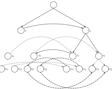
We can view the sets of equations defined in Definition 2.2 as tree-like graphs. Nodes correspond to variables. We first add a dummy root node with outdegree 2 whose children are the initial nodesx andy. The summation equations are represented by downward edges, from every parent node to its two children. We represent the multiplication equations as lateral edges, i.e., edges between nodes at the samelevel, i.e., distance from the root node. (Thus the graph is not really a tree if lateral edges are considered.). Because all left multiplication edges gotoT and have no effect on the complexity of the algorithm in these systems of equations, we leave these edges out of the diagrams for clarity. LetG(n) be the graph ofσ(n)See Figure 1 forG(0). Note that the height of the tree is 3, i.e, there are 3 levels.
In general, the graph ofσ(n)hasn+3 levels. We view the algorithm as proceeding down the tree, with
x12 x11
y1 y2
x2 x1
y x
Figure 1: Example graph with a peak at nodex
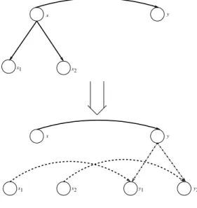
y x
x1 x2
y x
x1 x2 y1 y2
Figure 2: Sum transformation
Note also that other than at the lowest level (depthn+3) the graph will have initially one multiplica-tion or exactly one edge between nodes at the same height in the graph. We can also see that the graph is partitioned between the left and right side orxandyside and that at level one, there is an edge fromxto y. However, at all other lower levels, the initial edge between nodes of the same level goes fromytox.
We can also see that given the graph as described above, each time the sum transformation is applied, the peak moves from either thex side of the graph to the y side or from theyside to the x side, and the new peak was not previously a peak. To see this, take any system as defined by Definition 2.2 and examine the graph of that system. Initially all edges from nodes at the same height only go from one side to the other. In this limited formulation of Definition 2.2 these same level edges are the only multiplication functions. This ensures that any time a sum transformation is performed on some equation, xi=?T×yj oryi=?T×xj, by definition the new edges created by the sum transformation must go from
eitherx toy ory tox because there are no multiplication equations of the formxi =? T×xj. The fact
transformation. Since we assume a simple system of equations, there are no two distinct equations of the formx=?x
i+xj, x=?xk+xl (i.e., with the same variable on the left-hand side): likewise for y. Once
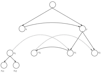
when the sum transformation is applied to equationsxi=?T×yjandxi=?xi1+xi2, the downward edges
fromxito bothxi1andxi2are removed (see Figure 3). Thusxican never become a peak again.
x12 x11
y1 y2
x2 x1
y x
Figure 3: Graph after one application of the sum transformation at nodex, creating a new peak at node x1and new edges fromx1toy1andx2toy2
Lemma 3.1. Sum transformations at level k create a peak at x1k at level k+1provided k+1is not the
lowest level.
Proof. This follows inductively from the form of the graph in Definition 2.2. First from the definition of the set of equations, the first peak is located atx. After the first sum transformation a peak is created atx1.
Assume this propagates to leveln. Then there is a peak atx1n to which the sum transformation is applied,
adding an equation of the formx1n+1 =?T×y1n+1, which creates a peak at the next level, provided there is already an equationx1i+1=?x1i+2+x1i+12.
Lemma 3.2. There are no lateral edges from nodes corresponding to variables of the form y2j for j≥0.
In other words, no equations of the form y2j =?T×xk are generated.
Proof. This follows inductively from Definition 2.2. In any initial system there is no edge from anyy2k
node at levelk. By the definition of sum transformation an outgoing lateral edge fromy2k can be created
only if the parent node,y2k−1 has an outgoing lateral edge.
We can also notice a fact about the order in which the nodes become peaks via the sum transforma-tion. The order is a right-to-left lexicographical order of the digits of the nodes’ indices (i.e., subscripts). For example, for level 4 the sequence isx111→y111→x211→y211→x121→y121→x221→y221→
x112→y112 →x212→y212→x122→y122→x222→y222. Note, y222 is not necessarily a peak but is
added to illustrate the path. Based on this observation we have the following lemma:
Lemma 3.3. At any level of the tree, if xi=? T×yj is an equation (i.e., if there is a lateral edge from
xi to yj) then i= j. Similarly, if yi =? T×xj is an equation, then j =revlex(i) where revlex is the
Proof. This follows inductively from Definition 2.2 and the sum transformation. The base cases are x=?T×y(level 1) andy
1=?T×x2(level 2). Assume this property for levelk. Now we will show that
all the equations introduced at levelk+1 by sum transformation at levelkwill satisfy the property. If yi=?T×xrevlex(i)is an equation at levelkandyi=?yi1+yi2is an equation (i.e.,yi is a peak at levelk),
then applying the sum transformation results inyi1=?T×xrevlex(i)1andyi2=?T×xrevlex(i)2. Now note
thatrevlex(i1) =revlex(i)1 andrevlex(i2) =revlex(i)2 sinceiis not a string of 2’s. Note also that ifk is not the lowest level, then there will already be an equationy2k1=?T×x1k2at levelk+1 but this does
not violate the property in the lemma sincerevlex(2k1) =1k2.
Ifxi=?T×yiandxi=?xi1+xi2, then by application of the sum transformationxi1=?T×yi1andxi2=?
T×yi2and the result follows.
Lemma 3.4. If there is a path of lateral edges from node uito node vi in the graph at some point where
node uiis a peak, then every node on the path, except possibly vi, will become a peak at some point.
Proof. Straightforward, by induction on the length of the path.
Lemma 3.5. At every level k<n+3a path of lateral edges between x1k−1 to y2k−1 is created.
Proof. For brevity, we refer to such paths as RL paths. Clearly there (already) is an RL path at level 1. We show that if a RL path exists at levelkandk+1<n+3, then a RL path will be created at levelk+1. By Lemma 3.1 there will be a peak atx1k−1 and by Lemma 3.4 every node other thany2k−1 will become a peak. This creates, at levelk+1, edges of the formxi1=?T×yi1,xi2=?T×yi2,yi1=?T×xrevlex(i)1
andyi2=?T×xrevlex(i)2 for everyi6=2k−1. Since the edgey2k−11=?T×x1k−12is already there to begin with, we get the RL path at levelk+1.
Lemma 3.6. At each level k<n+3of the graph, the sum transformation can be applied2k−1times.
Proof. Follows from Lemma 3.5. At each levelk, 2knodes will be created eventually. An RL path can
be created and thus the sum transformation must be applied to all nodes excepty2k−1 resulting in 2k−1 applications at each levelk.
Theorem 3.7. For a graph of height n,2n+1−n−2sum transformations are used.
Proof. This easily follows from Lemmas 3.1– 3.6 and the fact that∑ni=0 2i−1
=2n+1−n−2.
4
An Illustrated Example
In this section we give an example of the process on a system of equations defined as in Definition 2.2. We begin withσ(0), i.e., the following set of initial equations:
x =? T×y,
x =? x 1+x2,
y =? y 1+y2,
y1 =? T×x2,
x1 =? x11+x12
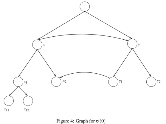
This can be represented by a graph as shown in Figure 4. Note that the first peak is located at nodex. The
x12
x11
y1 y2
x2
x1
y x
Figure 4: Graph forσ(0)
first peak,x, is selected and the sum transformation can be applied, resulting in the removal of equation x=?x
1+x2from the set of equations and the addition of the two equationsx1=?T×y1andx2=?T×y2.
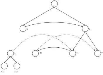
The direction of the new edges are fromxtoydue to the fact that the multiplication equation from the peak, to which the sum transformation was applied was also fromxtoy. After the sum transformation is appliedxis no longer a peak because of the removal ofx=?x
1+x2, but now the nodex1is a peak due
x12 x11
y1 y2
x2 x1
y x
Figure 5: After one application of the sum transformation
We see that only one application of the sum transformation can be applied at level 1. At the next level we continue the process begining with the new peakx1. The result of applying the sum transformation
on x1 is the removal ofx1=? x11+x12 from the set of equations and the addition of two new edges,
x11=?T×y11andx12=?T×y12, to the set of equations. The two newynodes are also created adding
y1 =? y11+y12 to the set of equations. The result is that x1 is no longer a peak but now y1 is (see
Lemma 3.3). The resulting graph can be seen in Figure 6. Also, now thaty1is the peak the direction of
the multiplication path has switched to the direction ofy1tox2(see Lemma 3.1).
x12 x11
y1 y2
x2 x1
y x
y11 y12
Figure 6: After two applications of the sum transformation
We can now continue the process, applying the sum transformation to the peak at y1. This will
removey1=?y11+y12fom the set of equations and addx2=?x21+x22to the set of equations, creating a
peak at nodex2and removing the peak at nodey1. Lastly, a third sum transformation is applied to node
x2, removingx2=?x21+x22from the set of equations and addingy2=?y21+y22to the set of equations.
Note that because there is no multiplication path fromy2 to somexnodey2is not a peak and no more
y1 y2 x2
x1
y x
x12 x21 x22 y11 y12 y21 y22
x11
Figure 7: After 4 applications of the sum transformation
5
Conclusions
We have shown that the Tiden-Arnborg algorithm does not run in polynomial time as claimed in [8]. It is also not hard to see that the algorithm produces exponentially largemgusfor the set of systemsσ(n).
However, it may still be that theunifiabilityproblem, i.e., whether a unifier exists modulo this theory, is inP. We are currently working on this and related problems.
References
[1] Siva Anantharaman, Hai Lin, Christopher Lynch, Paliath Narendran & Micha¨el Rusinowitch (2010): Cap unification: application to protocol security modulo homomorphic encryption. In: Dengguo Feng, David A. Basin & Peng Liu, editors: ASIACCS, ACM, pp. 192–203. Available athttp://doi.acm.org/10.1145/ 1755688.1755713.
[2] Franz Baader & Wayne Snyder (2001): Unification Theory. In: John Alan Robinson & Andrei Voronkov, editors:Handbook of Automated Reasoning, Elsevier and MIT Press, pp. 445–532.
[3] Evelyne Contejean (1993):A Partial Solution for D-Unification Based on a Reduction to AC1-Unification. In: Andrzej Lingas, Rolf G. Karlsson & Svante Carlsson, editors: ICALP,Lecture Notes in Computer Science
700, Springer, pp. 621–632. Available athttp://dx.doi.org/10.1007/3-540-56939-1_107.
[4] Evelyne Contejean (1993):Solving *-Problems Modulo Distributivity by a Reduction to AC1-Unification. J. Symb. Comput.16(5), pp. 493–521.
[5] Jean-Pierre Jouannaud & Claude Kirchner (1991): Solving Equations in Abstract Algebras: A Rule-Based Survey of Unification. In:Computational Logic - Essays in Honor of Alan Robinson, pp. 257–321.
[6] Hai Lin (2009):Algorithms for Cryptographic Protocol Verification in Presence of Algebraic Properties. Ph.D. thesis, Clarkson University.
[7] Manfred Schmidt-Schauß (1998): A Decision Algorithm for Distributive Unification. Theor. Comput. Sci.
208(1-2), pp. 111–148. Available athttp://dx.doi.org/10.1016/S0304-3975(98)00081-4.
[8] Erik Tid´en & Stefan Arnborg (1987):Unification Problems with One-Sided Distributivity. J. Symb. Comput.