nade Liberalization and the Evolution of Skill
Earnings Differentials in Brazil
*
Gustavo Gonzaga
PUC-llio
N aércio Menezes Filho
USP
JEL classification: F13, J31
Cristina Terra
EPGE-FGV
Keywords: Earnings inequality, trade liberalization
September 27, 2002
Abstract
From 1988 to 1995, when trade liberalization was implemented in Brazil, relative earnings of skilled workers decreased. In this paper, we in-vestigate the role of trade liberalization in explaining these relative earn-ings movements, by checking all the steps predicted by the Heckscher-Ohlin-style trade transmission mechanism. We find that: i) employment shifted from skilled to unskilled intensive sectors, and each Sector increased its relative share of skilled labor; ii) relative prices fell in skill intensive sectors; iii) tariff changes across sectors were not related to skill inten-sities, but the pass-through from tariffs to prices was stronger in skill intensive sectors; iv) the decline in skilled eamings differentials mandated by the price variation predicted by trade is very elose to the observed one. The results are compatible with trade liberalization, accounting for the observed rei ative eamings changes in Brazil.
1
Introduction
In terms of income distribution, Brazil is one of the most unequal countries in
the world. In the Human Development Report (United l\ations Development
Program, 2000), for example, Brazil tops the ranking of income concentration
°The authors are grateful to Honório Kume for providing tariff data: Maurício :Mesquita
for 86 countries in the world. The ratio between the mean income appropriated
by the richest 20% of families and by the poorest 20% is about 33 in Brazil,
compared, for example, to 8 in the U.S., 9 in the U.K., 14 in Russia, 4 in Sri
Lanka and Nepal, 18 in Kenya and 30 in Guatemala (the country with the second
highest ratio). Squire and Zou (1998) also present data on Gini coeffi.cients for
several countries, which show Brazil on the top of the list with an average (over
time) coefficient of 0.578 relative to a sample mean (s.d.) of 0.362 (0.092).
The leveI and dispersion of wages in a country at a point in time in general
depend on the distribution of its workers' characteristics, such as education,
effort, experience, other observed and unobserved skills, and on the returns to
these attributes. These returns, in turn, depend on the demand distribution for
these characteristics. Institutional factors, such as trade unions and minimum
wages, may also affect the wage structure. In Brazil, as well as in other less
developed countries, education is often seen as the main source of inequality.
Barros et ai (2000), for example, show that the distribution of education and its returns account for about half of the wage inequality from observed sources in
Brazil. This occurs because education is very unequally distributed and because
returns to education are quite high in Brazil.1
Although income inequality has not changed much over the past fifteen years,
education earnings differentials fell during the trade liberalization period. Brazil carried out a massive trade liberalization from 1988 to 1995. Non-tariff barriers
were first gradually substituted by tariffs, and then tariffs were reduced from
an average of 39.6% in 1988 to 13.1 % in 1995. Earnings of workers with at
least high school diplomas were 3.85 times higher than those for less educated
workers in 1988, and this ratio decreased to 3.28 in 1995.
This paper investigates the role of trade liberalization in explaining these
relative earnings movements, through a Heckscher-Ohlin-style mechanism. This
is accomplished by performing several independent empirical exercises,
includ-ing consistency checks on the causality path predicted by trade theory, usinclud-ing
disaggregated data on tariffs, prices, wages, employment and skill intensity from
1988 to 1995. We produce evidence showing that trade liberalization played a
major role in accounting for the reduction of education earnings differentials in
Brazil between 1988 and 1995.
Brazil is particularly well suited for studying the effects of trade on
earn-ings inequality. First, Brazil moved from being a very protected economy to
an open one in a relatively short period of time. Second, relative prices have
displayed substantial variation over this period, mostly due to very high
infia-tion rates (the average monthly infiainfia-tion rate for. the 1988-95 period was 20,7%).
This is important because Stolper-Samuelson effects work through relative prices
changes. Finally, Brazil has very high-quality and relatively unexplored
estab-lishment and household data sets.
There is a wide empiricalliterature studying the contribution of international
trade to the rising skill premium in the D.S. and C".K., given the considerable
increase in trade over the past decades. Most of this literature is based on
the Heckscher-Ohlin model (see, for example, Lawrence and Slaughter, 1993,
and Leamer, 1996)), but a competing view attempts to associate the rising skill
premium to skill biased technological changes (see, for example, Berman, Bound
and Griliches, 1994, and Katz and Autor, 1999). Although some papers have
been successful in relating relative product prices changes to relative wages, most
of the available evidence favors the skill biased technological change explanation
(see Slaughter, 1998, for a survey of product-price studies using D.S. data).
With respect to less developed countries, the literature is far scantier (see
Slaughter, 2000, for a survey on the effects of trade liberalization on labor
countries have al50 experienced increases in wage differentials, despite having
opened their economies to trade. Hanson and Harrison (1999) argue that trade
protection was skewed towards low-skilled workers in Mexico prior to the reform,
50 that the tariffs decline was deeper in those sectors, which could have led to
the increase in wage differentials observed in this country. However, the authors
did not find any correlation between price changes and skill intensity. Robertson
(2001) shows that, following Mexico's entrance to the GATT, the relative price
of skill-intensive goods rose and 50 did the relative wages of skilled workers.
However, following the creation of NAFTA, the opposite took place. Beyer et
al.(1999) find that a falI in the relative price of labor intensive goods in Chile
helps to explain the simultaneous rise in wage inequality. This led Berman
et ai (1998) to argue that skill biased technological change was pervasive in
developing countries as well.
All studies on developing countries identify an increase in earnings
inequal-ity. This contrasts with the evidence for Brazil, where a decrease in earnings
differentials was observed. Moreover, there are no studies exploring the
Stolper-Samuel50n effects of trade on skilled earnings differentials through relative prices
in Brazil (see Arbache, 2001, for a survey on the effects of trade liberalization
on the Brazilian labor market).
A possible problem with the studies for other developing countries is the
use of the share of non-production workers as a proxy for skill intensity. As we
argue in Section 2, we consider education attainment a more adequate measure
of skill. Krueger (1997) uses both education and non-production share measures
of skill intensity for V.S. data, where both measures are available, and obtains
qualitatively the same results. Slaughter (1998) shows that the results of studies
that use either measure are comparable. This paper shows that this is not the
case for Brazil. When education attainment is used to measure skill intensity,
for the nonproduction measure. We show that both movements are compatible
with traditiona! trade theory. This should be taken as a warning for how to
interpret the results of studies for other developing countries.
The paper is organized as follows. Section 2 presents the data and some
stylized facts. The Brazilian trade liberalization process is briefiy described
in Section 3. Section 4 presents the various empirical exercises linking trade
libera!ization to earnings differentia!s and Section 5 concludes.
2
Data and Stylized Facts
We put together data from severa! different sources. For the education and
earnings data we use a particularly rich data set, consisting of repeated
cross-sections of an annua! household survey (Pesquisa Nacional de Amostras por
Domicílio - PNAD), conducted each September by the Brazilian Census Bureau
(IBGE) and used in severa! studies about the Brazilian labor market (see Lam
and Shoeni, 1989, for example). Each cross-section is a representative sample of
the Brazilian population and contains about 100,000 observations on households,
from which around 330,000 individuais are interviewed.
From the origina! data, we kept only individuais with positive hours worked
In the reference week and with positive monetary remuneration. The main
variable used in this ana!ysis is real hourly earnings, defined as the norma!
labor income in the main job in the reference month, norma!ized by norma!
weekly working hours. The sample also includes self-employed and workers
with informal contrac~. We measure education by completed years of formal
schooling.
We split individuais into two education groups: the skilled (those that have
at least completed high school, that is, 11 years of education) and the unskilled
1,8,
1,7 -'
-1,1---~e-·~'~Q
- collega definition - - - high schooI definition •• <> •• manutacturing onJy
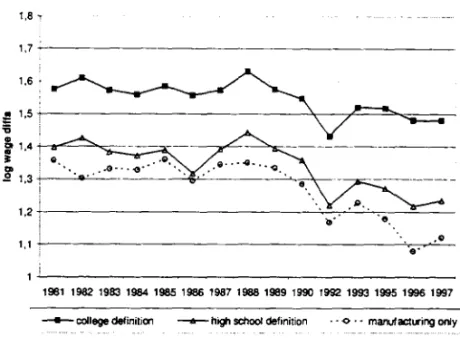
Figure 1: Education Earnings Differentials
than 10% of the workforce had completed college education over the period
studied, which is cIearly toa small a fraction of the labor force, compared with
more than 20% of workers with complete high school. Therefore, we choose to
use the high school definition in alI empirica! exercises that follow.
Figure 1 shows the evolution of earnings differentials between skilled and
unski11ed workers in Brazil between 1981 and 1997. The dotted line uses our
preferred measure of ski11 (high school or more) and refers to the manufacturing
sector only. It shows that wage differentials remained basica!ly constant between
1981 and 1988, dropping continuously afterwards. It is important to note that
trade liberalization started in 1988. The continuous line with triangles shows
that the behavior for the economy as a whole fo11owed a similar path, which is to
be expected, as workers can move between sectors. Finally, the line with squares
shows what happens if we use college education to define a skilled worker. The
magnitude and concentrated in the 1988-1992 period2 .
As we mentioned in the introduction, all studies that investigated the effects
of trade liberalization in developing countries used the share of non-production
workers as a proxy for skill intensity. In order to compare our results with
those using this alternative definition, we used data on occupation from the
Brazilian Industrial Surveys (Pesquisa Industrial Anual-PIA), al50 collected by
the Brazilian Census Bureau over the same time period, and matched them
to the education definitions described above. As the sectors in the industrial
surveys are defined at a more disaggregated leveI than in the household surveys,
we would obtain efficiency gains by using the non-production definition of skill
if the results using the two definitions of skill were compatible.
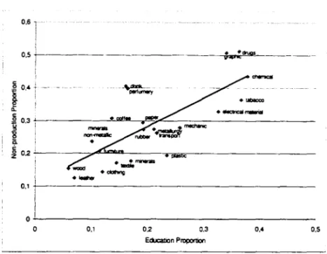
Figures 2 and 3 show that, while there is a strong as5Ociation between the
high education and the non-production employment share across the
manufac-turing sectors, the correlation between the skill earnings differentials computed
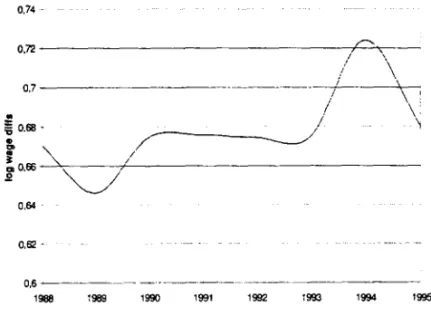
using the two definitions is much weaker. More importantly, Figure 4 shows
that the earnings differentials computed using non-production occupation as a
proxy for skill actually rose slightly along the sample period. This behavior
contrasts with the falI of relative earnings observed when education attainment
is used as a proxy for skill. Obviously, neither measure perfectly refiects skill
intensity, which is unobservable to the econometrician. Education attainment
fails to refiect skill intensity when, for instance, a highly educated worker is
per-forming a task that does not require skill. On the other hand, some blue-collar
workers can have highly skill demanding assignrnents. l\'onetheless, we believe
that education attainment is a more accurate proxy for skill. Based on these
considerations, we use education to construct our skill composition measure in
the empirical exercises that follow, but also report results of experiments using
0.6
0.5~--f
0.4o.. c:
--.1-.:0
i
0.3 ti _ _ _ _ _----X."""''---,~~----=:;:-:---i
K
.
~O~~·---~~~~--_.~~---01+-1 _ _ _ ·_---_ _ _ _ _ _ _ _ _ _ _ _ _ _ _ _ _ _ _
• I
I
I
0~1---O 0.1 0.2 0.3 0.4 0.5
Figure 2: Education and Ocupation Employment Shares
the occupation measure.
The drop in skilled-Iabor relativc earnings obscrved in Figure 1 could havc
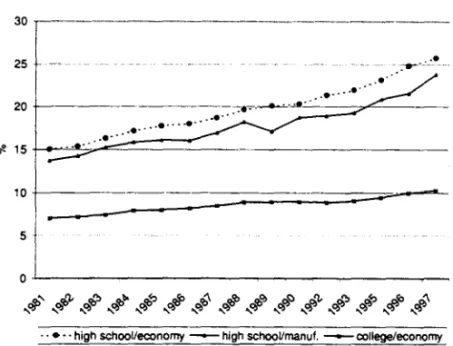
been caused solely by a rise in skilled labor relative supply. Figure 5 indeed
shows that there was a rise in the share of skilled workers over the same time
period, both in the manufacturing sector (line with triangles) and in the
econ-omy as a whole (dotted line). The line that uses the college definition of skill
(continuous with squares) also trended upwards, but at a slower pace. Note
that, according to the college definition, only about 9% of the workforce was
skilled in 1988-1995.
While labor supply could have a say in the decline of wage differentials
observed above, it is worth noting that the relative supply of skilled workers
rose steadily over the period. with minor fluctuations. By contrast, Figure 1
shows that wage differentials remained basically stahle Wltil 1988, starting to
~
"
2
-1.8 ;
.-
..
.
...
-1.6 - - - . - . - - - -_ _ _
.
...,
.-~,.4~
.~
~
ª
. - -
,...
.CClfI.. • ...
õil.2l~ ..,.,
~ I
W I • mKha'Ic
~ .~.'-Qi' .~
...
.,
...
0.8~!---~.n'mmo.Dr---0.6
0.2 0.4 0.6 0.8 1.2 1.4
ClcCI.pI1icn Wage Oiffs
Figure 3: Education and Occupation Earnings Differentials
0.74 .
0,72 _________________________________ /"',0=-::"',_, -~
I
\
.
~ Me
-I \
! \ ~
!
\
I '\
~~/
& / ~
;
""
/'" 0,66 -~,,---+ I'
'---.S! " - - . /
0.7 .
-0,64 .
0,62
-0,6 - - - . _ -..
1988 1969 1990 1991 1992 1993 1994 1995
30
---~---25 ~
..
.•
F"~.~
•.•.•..~;;2
. . . .
~
....•...~~
20
+---'$. 15 ~
-5
..••. high school/economy - high schooUmanuf. - - oollege/economy
Figure 5: Education Relative Labor Supply
that other factors are behind the behavior of wage differentials. We now try to
uncover these factors~
3
Theoretical Considerations
In traditional trade models, international trade is based on differences among
countries, which may be either in their factor endov.'Inents, as in the
Heckscher-Ohlin framework, or in the technology they possess, as in Ricardian models.
A common feature in these models is that, in a small open economy, relative
wages are a function only of technological parameters and relative prices. The
intuition for this result is the following~ In a small open economy, relative prices
of tradable goods are determined abroad, and any excess supply or demand is
fulfilled by trade of goods. Wages. in turn, are equal to the value of the
fac-tors' marginal productivity. As prices are exogenous, and marginal productivity
and technologica1 parameters, and not on factors' supply or goods' demand
parameters.:l
The crucial point in these models is that the effect of trade liberalization
on relative wages happens through its effect on relative domestic prices. In the
small country case, domestic prices are distorted by trade constraints, so that:
(1)
where Pi represents the domestic price for good i; ti is the import tariff or the
export subsidy (or more generally, any type of rents generated by other trade
barriers, like quantitative restrictions); Eis the nominal exchange rate; and Pt
is the international price of good i. The parameter ai captures the pass-through
from tariffs to domestic prices. In a H-O world, economies' trade is completely
specialized, that is, countries should import on1y goods in which they do not
have comparative advantage. In such a world, import tariffs' pass-through to
prices, ai, should be equal to one in the importing sectors and zero in the
exporting ones. There is no such complete specialization in the real world, as
not on1y H-O forces are in play. Hence, there will be imports and exports in alI
sectors. However, the sector in which the country has no comparative advantage
should present a higher pass-through from tariffs to prices.
Relative domestic prices are, thus, given by:
(1
+
tit
iPt
(l+tjt'Ij'
(2)Equation (2) shows that a falI in tradc barricrs across sectors may causc
changes in relative prices. This depends on the change in reIative tariffs and
3More precisei)'. if the economy is in the cone of diversification and the number of goods is greater ar cqual to the number of factors. then factor rclativc prices depcnd only on rclative priccs of tradablc goods bcing produced. and technological parametcrs. If the economy is outside the divcrsification cone. or the numbcr of goods is smallcr than the number of factors. then relativc factor priccs ",ill dcpend not onl)' on technology and rclativc priccs of goods being produced, but also on taste parameters and factor supplies. The existence of non-tradable goods does no! alter the main implications of the analysis. The uni)' effect of non-tradables
on the pass-through coefficients. If the pass-through is the same for alI sectors,
trade liberalization affects relative prices only if tariff reductions are
heteroge-neous across sectors. However, even a homogeheteroge-neous tariffs decrease may lead to
relative price changes, which happens when pass-through coefficients are
differ-ent.
If falling tariffs had a larger impact on prices of sectors that use skilled
labor more i ntensively, the new price incentives would then induce a shift of
production from skill- towards non-skill-intensive sectors, increasing the demand
for unskilled labor and decreasing that for skilled labor. In this case, for a given
labor supply, relative skilled-Iabor wages would decline in order to restore labor
market equilibrium.
The new relative wages, in turn, would induce producers to decrease the
use of the production factor that became relatively more expensive. Hence,
producers in each sector would change the mix of factors, using more skilled
and less unskilled labor relative to the pre-liberalization choice. This last effect
would offset the original relative demand increase for unskilled labor. In the
end, one should observe higher relative wages for unskilled labor, an increase
in employment and production in unskilled-intensive sectors, and an increase
in the use of skilled labor in alI sectors. The empirica! section of this paper,
Section 5, investigates whether the comovements of sectorial variables following
Brazilian trade liberalization conform to this trade transmission mechanism.
4 Trade Liberalization in Brazil
In this section we briefty describe the process of trade liberalization in Brazil.
Brazil has a long traclition of restrictive trade policies. From World War II to
1973 the country pursued an import substitution strategy, following the trend
mar-ket protection and subsidies to chosen industries. nom 1960 to 1973 there
was a gradual import liberalization, combined with export promotion policies,
inc1uding frequent exchange rate devaluations. As a result of these policies,
Brazilian exports became considerably more diversified. For example, coffee
exports, which accounted for 40% of total exports in 1964, fell to only 20% in
1973. The impact on imports was not as significant. There was some import
substitution in intermediate and capital goods, but imports remained highly
concentrated in those goods, as well as in oil, which accounted for 20% of total
imports in 1974.
The two oil crises of the 1970s brought about large trade imbalances. The
Brazilian government chose to use restrictive trade policy instead of letting
exchange rate devaluations restore trade balance. Tariffs and non-tariff barriers
were imposed, along with export promotion policies to compensate for the
anti-export bias generated by the import restrictions. The debt crisis of the 1980s
called for large trade surpluses, which were attained by the intensification of
trade restrictions and an industrial policy that gave fiscal incentives and cheap
credit to selected firms.
In sum, trade barriers were built over several decades, but responding to
dif-ferent policy orientations. Trade policy before 1974 was designed as an incentive
to selected sectors as part of the import substitution strategy. After 1974, the
increase in both tariff and non-tariff barriers was a reaction to macroeconomic
instability caused by the oil shocks and the debt crisis. The effect of these
poli-cies on relative prices distorted microeconomic incentives. By the end of the
1980's a maze of policy incentives was in place.
An important question for our purposes is whether the tariff structure
fa-vored skill-intensive sectors. In order to answer this question, we use data on
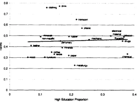
tariffs for 60 sectors between 1988 and 1995, from Kume et aI (2002). Figure
0.8
-.c::icIItq .â1nk
0.7 .
*0.6
-*_ ..
-0.5 - - - -.... .::...--... > - - - -... .",_---.-...
---<.'""""' ...
= ...
r-=l"'*--.
"'-=
...
~"i 0,4 _ _ _ _ _ _ _ L!!III!!L _ _ _ _
--r;.
~
>-*""fw
0,3 "",. ---~ .... __
-_.Jw! ...
__ : .... -___
.:...*"'-""_ _ _ _ _ _ _ _ _ _ ~ 0 2-0.1 •
o~·---0,1 02 0,3 0,4
HigI1 EdL<:alion Propomon
Figure 6: Tariffs and Skill Proportion
relation with skill-intensity (using education as a measure of skill). This comes
as no surprise, given that trade barriers were raised to cope v:ith
macroeco-nomic problems, and not to protect sectors in which Brazil had no comparative
advantage,
The trade liberalization process was initiated in 1988 and intensified by a new
government in 1990, in conjunction with the implementation of a regional trade
block, Mercosul.4 Trade liberalization was even deeper than planned, However,
after the 1994 Mexican crisis, there was a partial reversal of the processo Some
quantitative import restrictions were temporarily re-introduced, and some tariffs
were raised. Nonetheless, the average tariff leveI was below 14% by I"ovember
1995. The bulk of trade liberalization occurred from 1988 to 1995, with minor
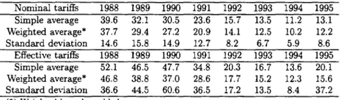
tariff changes since then. Table 1 shows the evolution of nominal and effective
tariffs from 1988 to 1995,
Nominal tariffs 1988 1989 1990 1991 1992 1993 1994 1995
Simple average 39.6 32.1 30.5 23.6 15.7 13.5 11.2 13.1
Weighted average* 37.7 29.4 27.2 20.9 14.1 12.5 10.2 12.2
Standard deviation 14.6 15.8 14.9 12.7 8.2 6.7 5.9 8.6
Effective tariffs 1988 1989 1990 1991 1992 1993 1994 1995
Simple average 52.1 46.5 47.7 34.8 20.3 16.7 13.6 20.1
Weighted average* 46.8 38.8 37.0 28.6 17.7 15.2 12.3 15.6
Standard deviation 36.6 44.5 60.6 36.5 17.2 13.5 8.4 37.2
(*) Weighted by value added.
Table 1: Nominal and effective tariffs, 1988-1995
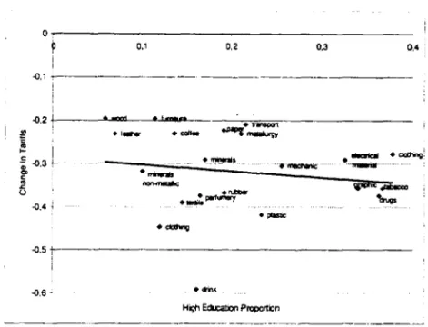
Figure 7 shows that tariffs seem to have declined slightly more in the more
skill-intensive sectors, although not dramatically so, a pattern that wiU be
fur-ther investigated below. This contrasts sharply with what was observed in
Mexico. Hanson and HarrisoIl (1999) and Robertson (2001), for example, show
that Mexican tariffs were relatively lower in skill-intensive sectors before trade
liberalization. and decreased less in those sectors.
5
Empirical Results
5.1 Within and Between Industry Decomposition
Our empirica! exercise begins by investigating whether trade liberalization is
the main reason for the drop in skill earnings differentials observed in Brazil or
whether the increase in skilled labor supply alone can explain it. As discussed
below, these two possible explanations have different implications for the
re-sults of standard decompositions of skilled-Iabor relative employrnent and wage
bill shares iuto within and between industry change (see Berman, Bound and
Griliches, 1994 and Autor. Katz and Krueger, 1998).
Changes in skilled-Iabor employment share
(~
(Ll:L> ))
may be0,1---~ 0.1 0.2 0.3 0.4 :
.Q.1 ,"""o
-.Q.2 +.-1 - - - ' . . . - - - -. . . . , , - - . . . .
'---.0==---~.-=
~ .
~
i
o; .Q.3 t~
U
• cdI ..
• """""sI
.~
".n'IIChanc:
_ • """""sI: ~"....--- .. '
.
...,
.Q.5~:---.Q.S·
HogIl Educa!Ion Propol1i>n
Figure 7: Changes in Tariffs and Skill ProportiOIl
which are interpreted as:
1. within industry changes, which are changes in skilled-Iabor employment
'within each industry (.6.
(Ll:LS )
J)' for a given employment share in each.
(Lu+L
S)mdustry (sJ = LL'+p!);
2. bctween industry changes. which are changes in each industry employment
share (.6.s)). for a given skilled-Iabor employment share in each industry
((Ll:LS )/
What would be the results of this decomposition exercise if the increase in
relative labor supply were the only significant change in the economy? According
to the Rybczynski theorem. for a small open economy, an increase in a factor
endowment raises the output of sectors that use that factor intensively, and
decreases other scctors' output, without changing the factor proportion uscd
represented by a positive left hand side. Since factor proportions do not change
in each industry, the first term on the right hand side, which represents the
within industry effect, should be zero. The whole effect should lie in the second
term - the between industry effect- which should be positive.
What would be the results of this exerci se if trade were the only source
behind the changes in wage inequality? As described in Section 3, trade should
have caused a decrease in relative prices of skill-intensive sectors in order to
produce the observed decrease in wage inequality. On the one hand, these
price incentives would decrease production in those sectors, which denote a
negative between industry effect. On the other hand, the relative wage incentives
would shift labor demand towards skilled workers within each industry, that is,
a positive within industry effect. With given factor supplies, the two effects
should offset each other. It is important to note, however, that skill biased
technological change would also cause a positive within industry effect. The
two effects would reinforce each other here, as opposed to the case in developed
countries.
Table 2 presents the decomposition results for skilled-Iabor employment and
wage bill shares, using education attainment as a measure of skill. Confirming
the labor supply movements displayed in Figure 5, skilled-Iabor employment
share increased 2.67% a year between 1988 and 1995, on average. The
de-composition reveals that the within effect is positive and the between effect is
negative. Two important conclusions emerge: (1) labor supply changes alone
cannot account for these results, and (2) the results are compatible .... ith the
trade explanation.5
Table 2 also shows that the wage bill share of skilled workers increased over
5 Results not rcported hcre. using non-production sharc as a proxy for skill. are also com-patible with trade. But in this casco the)" explain the increase in earnings differentals obscrvcd
for that skill mcasure. Thcrc was an avcrage ovcrall annual decrease of 0.7% in non-production employmcnt share. This W~ dccomposcd into a IIcgativc withm industry effcct (-lAVo). which
High Education Employment Share
High Education Wagc Bill Share
Total 0.0267 (100%)
0.0084 (100%)
Within Sectors 0.0334 (125%)
0.0256 (304%)
Between Sectors -0.0067
(-25%)
-0.0172 (-204%)
Table 2: Employment and Wage Bill Shares Decompositions, 1988-95
the period. However, it increased on average less than the employment share,
0.84% by year. This is compatible with the observed decrease in skilled labor
relative wages. Con..<;equently, the skilled worker wage bill share between sector
effect is larger compared to that of employment share. The employment share
decomposition presents a negative between efJect, which means that, on average,
employmcnt share decrcascd in industrics that use skil1cd labor more intcnsivcly.
As these sectors use more of the factor that had its remuneration decreased, it is
logical that their overal1 wage bill share should decrease by a larger proportion
than the employment share.
5.2 Consistency Checks
In this sub-section, consistency checks examine the causality path predicted by
tradc thcory. .t>,.s discussed in Scction 3, thc following rclationships should be
investigated to determine whether trade liberalization was responsible for the
decrease in skil1ed labor relative earnings observed in Brazil:
1. W'hat was the pattern of relative price changes? To be consistent with the
decrease in earnings inequality, one should observe a decrease in the
rela-tive prices of the sectors that use skilled labor intensivcly. This should be
refiected in the data through a negative correlation between price changes
and skill intensity.
2. Was the pattern of price changes caused by tariJJ changes? This can be
rela-tionship established in equation (1). If the changes in relative prices in
skill-intensive sectors were induced by trade liberalization, one should
ei-ther observe that the largest tariff reductions occurred in the most
skill-intensive sectors or that the effect of tariffs on prices was larger in these
sectors.
5.2.1 Prices, Tariffs and Skill Intensity
The first step is to check whether the pattern of price changes is consistent with
the observed decrease in skilled labor relative wages. We start by estimating
the following equation:
610g Fi.,.
=
80+
(3110g(LU LS LS) .
+
lIi.,.,+
t,"'-l(4)
where Fi.,. is the wholesale price for sector i in year T. The pattern of price
changes must deliver a negative value for (31' in order to be consistent with
the decrease in skilled-labor relative earnings. Before turning to the estimated
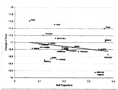
equations, Figure 8 shows that, between 1988 and 1995, prices rose less in sectors
with a higher proportion of educated workers.
Equation (4) is cstimated usinga panel of yearly observations from 1988
to 1995, for a sample of 60 sectors, defined according to the Brazilian
Indus-trial Surveys (PIA). The Brazilian wholesale price index (Índice de Preços por
Atacado, IPA) was collected by the Getulio Vargas Foundation and was made
compatible with the PIA sectorial definitions. We correct the standard errors
of ali coefficients here and in the following sub-section for the fact that our
independent variable (share of educated workers) is more aggregated than the
dependent variables we use.
The results of estimating equation (4), with annual data and controlling
for time effects, are presented in the first three columns of Table 3. A
18
1
I17'81
17,6 I
17,4+-.--
---
.-I
.-
,-~ 17.2 +-1 ---4~- _ _ _ _ _ _ _ _ _ _ _ _ _ _ _ _
!t ; • J*fllJW)' tmaxo
<.l
.~~
.. -161,78~1 ==~;;:5~~==::·
=
:::-
.
--;;; • • • êdf .....,.~ .~
-:..~:...
.ce.:
16,6
t ..
16,4 t
16,2 T .-..:;;
_ _ o
I _
16~1---
__________ ___
°
0,1 0,2 0,3 0,4SkiI Prcportions
Figure 8: Price Changes and Skill Proportion
showing that rclative prices changed in favor of less skill-intensive scctors, In
the second column, we include the share of non-production workers as an
addi-tional contro!' which attracts a negative coefficient and significantly raises the
estimated education share coefficient. This suggests that the two skill measures
are positively correlated with each otheL but relative prices rnoved in opposite
directions with respect to them, 50 that the exclusion of one measure biases the
coefficient of the otheL In the third column, we do not use the employment
weights, v.rith no observed qualitative change in the results, Therefore, relative
price changes are consistent with the observed change in earnings differentials,
According to our story, the Heckscher-Ohlin trade transmission mechanism
is triggered by a reduction in trade barriers that have different impact across
sectors, This could be the result of either a ::;harper reduction in tariffs in more
skill-intensive sectors or a larger impact on prices of the tariffs redllction in these
sectors. We investigate the first possibility here. while the second is exarnined
20
in the next sub-section.
We estimate the correlation between tariff changes and skill intensity using
the following equation:
~log(1
+t)i7"=
lO+'1
10g(LU LS LS).
+1]i7"'+
'.7"-1(5)
whcre ti stands for tariffs in sector i. and
(Ll:LS ) ;
is the share of skilled laboremployed in sector i.
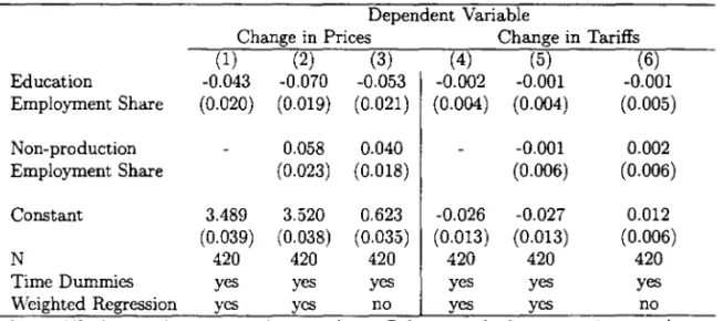
The results are presented in columns (3) to (6) in Table 4. Ncither skiU
inten-sity measures are significantly correlated with the changes in tariffs. Therefore,
as suggested by Figure 7, there is no clear pattern of tariff reductions with
relation to skill intensity in Brazil.
Dependent Variable
Change in Prices Change in Tariffs
(1) (2) (3) (4) (5) (6)
Education -0.043 -0.070 -0.053 -0.002 -0.001 -0.001
Employment Share (0.020) (0.019) (0.021) (0.004) (0.004) (0.005)
Non-production 0.058 0.040 -0.001 0.002
Employment Share (0.023) (0.018) (0.006) (0.006)
Constant 3.489 3.520 0.623 -0.026 -0.027 0.012
(0.039) (0.038) (0.035) (0.013) (0.013) (0.006)
N 420 420 420 420 420 420
Time Dummies yes yes yes yes yes yes
Wcighted Regression ycs ycs no yes ycs no
Kotes: Weights are the sector employment shares. Robust standard errors are in parentheses
Table 3: Tariffs and Skill Intensity, 1988-95
5.2.2 Prices and tariffs
From equation (1), domestic prices changes are related to changes in trade
~logPir
=
O:i~log (1+
tir)+
~logE+
~logP;~. (6)Since the nominal exchange rate is the same for every sector, and data
on rents generated by other trade barriers is unavailable, the equation to be
estimated takes the following form:
~logPir
=
150+
c510:i~log (1+
Tir )+
c52~logPi~+
éi (7)where Ti is the import tariff for sector i, and U.S. prices are used as a proxy for
international prices
P;*.
Changes in the nominal exchange rate are a componentof the constant term, 150 ; whereas changes in the rents generated by other trade barriers are captured by the error term, éi. The expected values for parameters
151 and 152 are 1. Remember that O:i is the pass-through coefficient from tariffs
to prices in sector i. We start by imposing that the pass-through coefficient be
equal in ali sectors (O:i = 0:, Vi), that is, we estimate the coefficient 1510:.
Equation (7) is estimated using a panel of yearly observations from 1988 to
1995, for the same sample of 60 sectors. U .S. producer price data were drawn
from the Bureau of Labor Statistics Website. We could only match 50 U.S.
sectors to the equivalent Brazilian sectors.
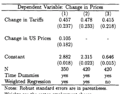
The first column of Table 4 presents the estimation results when changes in
tariffs and in U.S. prices are used as explanatory variables for price changes in
Brazil. The estimated tariff coefficient is positive and significantly different from
zero at conventional statistical leveis. However, the coefficient for U.S. prices
is not precisely estimated. This might indicate that U .S. prices are a poor
proxy for international prices. Therefore, in column (2) we drop C.S. prices to
gain efficiency, but the results do not change qualitatively. Finally, in the third
column we use an unweighted regression and show that the results are robust to
together for the period as a whole.
Dependent Variable: Change in Prices
(1)
(2)
(3)
Change in Tariffs 0.457 0.478 0.415
(0.237) (0.233) (0.218)
Change in US Prices 0.105 (0.182)
Constant 2.882 2.315 0.646
(0.018) (0.023) (0.015)
N 350 420 420
Time Dummies yes yes yes
Weighted Regression yes yes no
Notes: Robust standard errors are in parentheses. Weights are the sector employment shares.
Table 4: Prices and Tariffs, 1988-95
There is one caveat in interpreting the results of this regression. Equation
(1) refers to goods prices, and in the empirical estimation we use sectorial prices.
The composition of goods within each sector may change over time, and this
change may be correlated with changes in trade policy. On the one hand, trade
liberalization may reduce or even eliminate domestic production of goods with
relatively high domestic production costs. On the other hand, new products may
be introduced due to the reduced cost of imported goods. Even though this is a
drawback thcrc is nothing wc can do to corrcct for possible mcasurcmcnt errors
caused by it.
\Ve now allow for a different pass-through coefficient across sectors. As
discussed above, although tariff changes and skill intensity showed no significant
correlation, it is still possible that relative price changes. which were consistent
with the relative wages changes, were caused by trade. This would be true if
reduction, albeit uniform across sectors, produced ditferentiated price responses.
In particular, the observed relative price changes could have been caused by the
trade liberalization if the pass-through coefficient from tariffs to prices were
higher in skill intensive sectors.
We therefore split the sectors in two groups according to their share of
ed-ucated workers: those with shares above the median in 1988 and those with
shares below the mediano We then interacted the changes in tariffs with these
group indicators. The results are presented in Table 5. In column 1, where we
include U.S. prices as an additional control, we can note that that coefficient of
the change in taritfs is almost one and a half times higher in the high education
sectors. This result is maintained if we drop D.S. prices, as column (2) shows.
More importantly, if we do not use the employment weights in the regression,
the difference in the pass-through coefficients increases substantially, to almost
5 times. We feel these results provide evidence in favor of the ditferent taritf
pass-through coefficient hypothesis.
5.3 Mandated Wage Equations
While the pattern of price changes is consistent with the pattern of relative
earn-ings evolution, and seems to be deterrnined by taritf changes, we have not as yet
examined how much of the drop in skill earnings ditferentials could be attributed
to price changes. We therefore folio\\' another vein of the trade literature (see
Baldwin and Cain, 1997, Haskel and Slaughter, 2002, and Robertson, 2001) and
estimate mandated wage equations. According to the Stolper-Samuelson
theo-rem, price changes should equal factor price changes, weighted by the factor cost
share. If the only factors of production used were skilied and unskilled labor, it
is easy to show that price changes could be decomposed in two terms:
OS S U
u
lllog Pj
= /
(lllog w - lllog w )+
lllog tu ,J
Dependent Variable:
Change in tariffs
*
Low Education Share Indicator
Change in tariffs
*
High Education Share Indicator
Change in US prices
Constant
N
Time Dummies Weighted Regression
Change in Prices
(1) (2)
0.393 0.402
(0.271) (0.269)
0.591 (0.311) 0.115 (0.184) 2.882 (0.018) 350 yes ycs 0.635 (0.303) 2.315 (0.024) 420 yes ycs
Notes: Weights are the sector cmploymcnt shares. Robust standard errors are in parentheses.
(3) 0.164 (0.261) 0.783 (0.265) 0.646 (0.01.5) 420 yes no
Table 5: Prices and Tariffs by Skill Intensity, 1988-95
where Of is the cost of skilled labor and O j is the total cost in sector j. Therefore,
regressing price changes on skilled labor cost share should yield an estimate of
the economy-wide returns to skill changes.
Our estimation is based on the following regression:
~logpj
=
<7)0+
<7)1(w
UL~S::SLS
) j+
Tlj· (9)where the estimated coefficient </>1 is interpreted as the changes in skill earnings
differentials associated with price changes6
Since we are interested in the effect of prices that resulted frorn trade
liber-6The general form for equation (8) when there are I factors of production is:
~logpi =..i 61 (~logwl - ~logw2) + _J 61+62 _ _ J ~logw2 +
L
I (6k
..2.~logwk)
.~ ~ k~ ~
In this case. one could stil! use equation (9). but the coefficient cPl should equal s [}
alization, we follow Haskel and Slaughter (2002) and estimate the equation (9)
in two steps. First, we estimate the change in prices predicted by the change in
tariffs. For this step, we compute two alternative sets of predicted prices: those
that result from the estimation of equation (7), presented in Table 4, and those
that result from allowing different pass-through coefficients according to sector
skill intensity, presented in Table 5. In the sec0!ld step, we estimate equation (9)
using the predicted prices, instead of actual prices, as the dependent variable.
In this case, the estimated coefficient q>l is interpreted as the changes in returns
to skill that are mandated by price changes induced by trade liberalization.
Dependent Variable: Change in Prices
Predicted Predicted by tariffs,
by tariffs diff. pass-through
(2) (3)
Education Cost Share -0.007 -0.029
(0.006) (0.006)
Constant 2.300 2.310
(0.003) (0.003)
Auxiliary Regrcssion Table 3 (2) Tablc 4 (3)
Actual Change in Wage Diffs -0.024 -0.024
N 420 420
Time Dummies yes yes
Notes: Weights used in the first three columns are the sector employment shares. Robust standard errors are in parcntheses.
Table 6: Mandated Wages
The results are presented in Table 6. The actual annualized fali in skill
earnings differentials observed in Brazil was 2.4% on average. The first column
shows that the decline in earnings differentials mandated by the price variation
predicted by the change in tariffs was estimated at 0.7%, but was not
signifi-cantly different from zero. However, when we use the price changes predicted
by tariffs, allowing for different pass-through coefficients (column 2), we find a
elose to the observed one.7 This result provides compelling evidence that trade
liberalization played a major role in explaining the decrease in skilled labor
relative earnings in Brazil.
6
Conclusion
During the trade liberalization implemented in Brazil from 1988 to 1995,
earn-ings of workers with at least complete high school decreased with respect to
earnings of less educated workers. In this paper we present evidence
compat-ible with trade liberalization having played a role in explaining these relative
earnings movements.
According to traditional trade theory, the mechanism through which trade
liberalization could have caused the observed reduction in relative earnings of
skilled workers in Brazil is the following. Trade liberalization should have
de-creased the relative prices of skill-intensive sectors, shifting production from
these to unskill-intensive sectors. This should have caused a relative decrease
in skilled labor demand, implying a fali in the relative wages of skilled labor .
The new factor price incentives, in turn, would have induced firms in ali sectors
to increase the proportion of skilled labor used in production.
We perform several independent empirical exercises that check this trade
transmission mechanism, using disaggregated data on tariffs, prices, wages,
em-ployment and skill intensity from 1988 to 1995. First, a decomposition analysis
of changes in skilled-Iabor employment share over this period reveals a positive
within industry effect and a negative between industry effect. This means that
employment shifted from skilled to unskilled intensive sectors, and that each
sector increased its relative share of skilled labor.
Second, a panel regression of prices on skill intensities delivers a negative
coefficient, which implies that relative prices indeed fell in skill intensive sectors.
Although tariff changes across sectors were not related to skill intensities, we
find that the pass-through from tariffs to prices was stronger in skill intensive
sectors. This is consistent with trade liberalization being responsible for the
relative fali in prices of skill intensive sectors.
Finally, we apply a mandated wage equation analysis. We show that the
decline in skilled earnings differentials mandated by the price variation predicted
Ttade Liberalization and the Evolution of Skill
Earnings Differentials in Brazil*
Gustavo Gonzaga
PUC-llio
N aércio Menezes Filho
USP
JEL classification: F13, J31
Cristina Terra
EPGE-FGV
Keywords: Earnings inequality, trade liberalization
September 27, 2002
Abstract
From 1988 to 1995, when trade liberalization was implemented in Brazil, relative earnings of skilled workers decreased. In this paper, we in-vestigate the role of trade liberalization in explaining these relative eam-ings movements, by checking ali the steps predicted by the Heckscher-Ohlin-style trade transmission mechanism. We find that: i) employment shifted from skilled to unskilled intensive sectors, and each sector increased its relative share of skilled labor; ii) relative prices fell in skill intensive sectors; iii) tariff changes across sectors were not related to skill inten-sities, but the pass-through from tariffs to prices was stronger in skill intensive sectors; iv) the decline in skilled earnings differentials mandated by the price variation predicted by trade is very elose to the observed one. The results are compatible with trade liberalization, accounting for the observed relative eamings changes in Brazil.
1 Introduction
In terms of income distribution, Brazil is one of the most unequal countries in
the world. In the Human Development Report (United Nations Development
Program, 2(00), for example, Brazil tops the ranking of in come concentration
for 86 countries in the world. The ratio between the mean income appropriated
by the richest 20% of families and by the poorest 20% is about 33 in Brazil,
compared, for example, to 8 in the V.S., 9 in the
u.K.,
14 in Russia, 4 in Sri Lanka and Nepal, 18 in Kenya and 30 in Guatemala (the country with the secondhighest ratio). Squire and Zou (1998) a1so present data on Gini coeflicients for
several countries, which show Brazil on the top of the list with an average (over
time) coeflicient of 0.578 relative to a sample mean (s.d.) of 0.362 (0.092).
The levei and dispersion of wages in a country at a point in time in general
depend on the distribution of its workers' characteristics, such as education,
effort, experience, other observed and unobserved skills, and on the returns to
these attributes. These returns, in turn, depend on the demand distribution for
these characteristics. Institutional factors, such as trade unions and minimum
wages, may also affect the wage structure. In Brazil, as well as in other less
developed countries, education is often seen as the main source of inequality.
Barros et
ai (2000), for example, show that the distribution of education and its
returns account for about half of the wage inequality from observed sources in
Brazil. This occurs because education is very unequally distributed and because
returns to education are quite high in Brazil.1
Although income inequality has not changed much over the past fifteen years,
education earnings differentials feU during the trade liberalization period. Brazil
carried out a massive trade liberalization ITom 1988 to 1995. Non-tariff barriers
were first gradually substituted by tariffs, and then tariffs were reduced from
an average of 39.6% in 1988 to 13.1% in 1995. Earnings of workers with at
least high school diplomas were 3.85 times higher than those for less educated
workers in 1988, and this ratio decreased to 3.28 in 1995.
This paper investigates the role of trade liberalization in explaining these
relative earnings movements, through a Heckscher-Ohlin-style mechanism. This
is accomplished by performing several independent empirica! exercises,
includ-ing consistency checks on the causality path predicted by trade theory, usinclud-ing
disaggregated data on tariffs, prices, wages, employment and skill intensity from
1988 to 1995. We produce evidence showing that trade liberalization played a
major role in accounting for the reduction of education earnings differentials in
Brazil between 1988 and 1995.
Brazil is particularly well suited for studying the effects of trade on
earn-ings inequality. First, Brazil moved from being a very protected economy to
an open one in a relatively short period of time. Second, relative prices have
displayed substantial variation over this period, mostly due to very high
infla-tion rates (the average monthly inflainfla-tion rate for.the 1988-95 period was 20,7%).
This is important because Stolper-Samuelson effects work through relative prices
changes. Finally, Brazil has very high-quality and relatively unexplored
estab-lishment and household data sets.
There is a wide empiricalliterature studying the contribution of international
trade to the rising skill premi um in the U.S. and U.K., given the considerable
increase in trade over the past decades. Most of this literature is based on
the Heckscher-Ohlin model (see, for example, Lawrence and Slaughter, 1993,
and Leamer, 1996)), but a competing view attempts to associate the rising skill
premium to skill biased technological changes (see, for example, Berman, Bound
and Griliches, 1994, and Katz and Autor, 1999). Although some papers have
been successful in relating relative product prices changes to relative wages, most
of the available evidence favors the skill biased technologica! change explanation
(see Slaughter, 1998, for a survey of product-price studies using U.S. data).
With respect to less developed countries, the literature is far scantier (see
Slaughter, 2000, for a survey on the effects of trade liberalization on labor
countries have also experienced increases in wage differentials, despi te having
opened their economies to trade. Hanson and Harrison (1999) argue that trade
protection was skewed towards low-skilled workers in Mexico prior to the reform,
50 that the tariffs decline was deeper in those sectors, which could have led to
the increase in wage differentials observed in this country. However, the authors
did not find any correlation between price changes and skill intensity. Robert5On
(2001) shows that, following Mexico's entrance to the GATT, the relative price
of skill-intensive goods rose and so did the relative wages of skilled workers.
However, following the creation of NAFTA, the opposite took place. Beyer et
al.(1999) find that a fall in the relative price of labor intensive goods in Chile
helps to explain the simultaneous rise in wage inequality. This led Berman
et ai (1998) to argue that skill biased technological change was pervasive in
developing countries as well.
All studies on developing countries identify an increase in earnings
inequal-ity. This contrasts with the evidence for Brazil, where a decrease in earnings
differentials was observed. Moreover, there are no studies exploring the
Stolper-Samuelson effects of trade on skilled earnings differentials through relative prices
in Brazil (see Arbache, 2001, for a survey on the effects of trade liberalization
on the Brazilian labor market).
A possible problem with the studies for other developing countries is the
use of the share of non-production workers as a proxy for skill intensity. As we
argue in Section 2, we consider education attainment a more adequate measure
ofskill. Krueger (1997) uses both education and non-production share measures
of skiU intensity for U.S. data, where both measures are available, and obtains
qualitatively the same results. Slaughter (1998) shows that the results of studies
that use either measure are comparable. This paper shows that this is not the
case for Brazil. When education attainment is used to measure skill intensity,
for the nonproduction measure. We show that both movements are compatible
with traditional trade theory. This should be taken as a warning for how to
interpret the results of studies for other developing countries.
The paper is organized as follows. Section 2 presents the data and some
stylized facts. The Brazilian trade liberalization process is briefiy described
in Section 3. Section 4 presents the various empirical exercises linking trade
liberalization to earnings differentials and Section 5 concludes.
2 Data and Stylized Facts
We put together data from several different sources. For the education and
earnings data we use a particularly rich data set, consisting of repeated
cross-sections of an annual household survey (Pesquisa Nacional de Amostras por
Domicz1io -PNAD), conducted each September by the Brazilian Census Bureau
(IBGE) and used in several studies about the Brazilian labor market (see Lam
and Shoeni, 1989, for example). Each cross-section is a representative sample of
the Brazilian population and contains about 100,000 observations on households,
from which around 330,000 individuaIs are interviewed.
hom the original data, we kept only individuals with positive hours worked
in the reference week and v,ith positive monetary remuneration. The main
variable used in this analysis is real hourly earnings, defined as the normal
labor income in the main job in the reference month, normalized by normal
weekly working hours. The sample also includes self-employed and workers
with informal contracts. We measure education by completed years of formal
schooling.
We split individuaIs into two education groups: the skilled (those that have
at least completed high school, that is, 11 years of education) and the unskilled
1,8 •
1,7 t--~
i
l,6i
~
~ l,5~!---~~V--~~~~~~--~
:a !
J
:::!
:.:::.~.~;s
1 2 + - - -_ _ _ _ a----'-.--= •••
~....,._'__.,IO~
..~
, 1t' a.
1,1 +-: - - -
."
1~'---
__ --______
~--- ccllege definilion _ _ high schooI definilion •• o .. manufact ... ing only
Figure 1: Education Earnings Differentials
than 10% of the workforce had completed college education over the period
studied, which is clearly too small a fraction of the labor force, compared with
more than 20% of workers with complete high school. Therefore, we choose to
use the high school definition in alI empirical exercises that follow.
Figure 1 shows the evolution of earnings differentials between skilled and
unskilled workers in Brazil between 1981 and 1997, The dotted line uses our
preferred measure of skill (high school or more) and refers to the manufacturing
sector only, It shows that wage differentials remained basically constant between
1981 and 1988, dropping continuously afterwards. It is important to note that
trade liberalization started in 1988. The continuous line with triangles shows
that the behavior for the economy as a whole followed a similar path, which is to
be expected' as workers can move between sectors. Finally, the line with squares
shows what happens if we use college education to define a skilled worker. The
magnitude and concentrated in the 1988-1992 period2.
As we mentioned in the introduction, ali studies that investigated the effects
of trade liberalization in developing countries used the share of non-production
workers as a proxy for skill intensity. In order to compare our results with
those using this alternative definition, we used data on occupation from the
Brazilian Industrial Surveys (Pesquisa Industrial Anual-PIA), also collected by
the Brazilian Census Bureau over the same time period, and matched them
to the education definitions described above. As the sectors in the industrial
surveys are defined at a more disaggregated levei than in the household surveys,
we would obtain effi.ciency gains by using the non-production definition of skill
if the results using the two definitions of skill were compatible.
Figures 2 and 3 show that, while there is a strong association between the
high education and the non-production employment share across the
manufac-turing sectors, the correlation between the skill earnings differentials computed
using the two definitions is much weaker. More importantly, Figure 4 shows
that the earnings differentials computed using non-production occupation as a
proxy for skill actually rose slightly along the sample period. This behavior
contrasts with the fall of relative earnings observed when education attainment
is used as a proxy for skill. Obviously, neither measure perfectly refiects skill
intensity, which is unobservable to the econometrician. Education attainment
fails to refiect skill intensity when, for instance, a highly educated worker is
per-forming a task that does not require skill. On the other hand, some blue-collar
workers can have highly skill demanding assignrnents. :'\onetheless, we believe
that education attainment is a more accurate proxy for skill. Based on these
considerations, we use education to construct our skill composition measure in
the empirical exercises that follow, but also report results of experiments using
0,6,
0.5 +--~ • ·ctucP
\li"'''
-f
0,4~ -~Q.
~ 0,3 i - _____
-~,-_.."'~""-~
--K
i02~1---~~~~----~~=--
.0,1
-
O~---°
0,1 0,2 0,3 0,4 0,5EóJcatIon Proponion
Figure 2: Education and Ocupation Employment Shares
the occupation mcasure.
Thc drop in skilled-labor rclativc earnings observed in Figure 1 could havc
been caused solely by a rise in skilled labor relative supply. Figure 5 indeed
shows that there was a rise in the share of skilled workers over the same time
period, both in the manufacturing sector (line with tríangles) and in the
econ-omy as a whole (dotted line). The line that uses the college definition of skill
(continuous with squares) also trended upwards, but at a slower pace. ~ote
that, according to the college definition, only about 9% of the workforce was
skilled in 1988-1995.
While labor supply could have a say in the decline of wage differentials
observed above, it is worth noting that the relative supply of skilled workers
rose steadily over the period, v.;th minor fluctuations. By contrast, Figure 1
shows that wage differentials remained basically stable until 1988, starting to
2
1.8
• '*"'-Y
1.6 + - - - -... ,"' ••••
._---.-_--,.--._~
•• • -_ _ o _ . • - ___ o _ _ _ _ o
.=
.coI'l . . ~• .-::w
...
.-0.8 - - - -... , _ _
-0.6.1....---·---.. - - - -.. - - - _ - - -_ _ · _ _ _ _ _ _ _
O 0.2 0.4 0.6 0.8 1.2 1.4
Figure 3: Education and Occupation Earnings Differentials
0,74 '
0,72
---7C'>.~"'--/
\
; \
0,7 - - -
/
\I
~g"
I
\
~/
t ""
/
",0,66 ' \ /
.2 '---../
0,64 .
0,62 - .
0 , 6
-1988 1989 199J 1991 1992 1993 1994 1995