Trade Liberalization and Industrial Concentration:
Evidence from Brazil
∗
Pedro Cavalcanti Ferreira Giovanni Facchini
Graduate School of Economics Department of Economics
Fundacao Getulio Vargas University of Illinois at Urbana Champaign
Rio de Janeiro, Brazil Champaign, IL 61820
email: ferreira@fgv.edu email: facchini@uiuc.edu
February 28, 2004
Version 1.0: Comments are welcome
Abstract
This paper applies an endogenous lobby formation model to explain the extent of trade protection granted to Brazilian manufacturing industries during the 1988-1994 trade liberalization episode. Using a panel data set covering this period, we find that even in an environment in which a major regime shift has been introduced, more concentrated sectors have been able to obtain policy advantages, that lead to a reduction in international competition. The importance of industry structure appears to be substantial: In our baseline specification, an increase in concentration by 20% leads to an increase in protection by 5%-7%.
JEL Classification: F13.
∗Some of the ideas of this paper were fostered during conversations with Boyan Jovanovic, to whom we
1
Introduction
Active trade policies are seldom justifiable on efficiency grounds. In most cases, they are
instead the result of distortions introduced through the political process. While a large
liter-ature has highlighted the role of organized groups in the provision of trade protection, only
few theoretical contributions have explicitly identified the link between industrial structure,
the process of lobby formation and the determination of trade policy. In this paper we use
Magee’s (2002) model to understand the recent Brazilian trade liberalization experience.
The case of Brazil is very interesting for a variety of reasons. First, although widely
discussed in the press, the role of lobbying by organized groups in shaping economic policy in
the large Latin American country has been the subject of only sparse studies (Olarreaga and
Soloaga (1998), Helfand (2000), Gawande, Sanguinetti, and Bohara (2003)). Secondly, the
generalized trade liberalization that took place between 1988–1994 has been a major policy
reversal, and represents a particularly challenging ground to test explanations of trade policy
based on the lobbying activity of organized interests groups. Third, the existing empirical
literature linking lobbying activity and industrial structure based on cross-sectional studies
(Baldwin (1985), Trefler (1993), Goldberg and Maggi (1999) etc.) has not reached clear–cut
conclusions on the role of industry structure in explaining protection. As Rodrik (1995)
points out
“High levels of concentration in the affected industry itself are apparently not
always conducive to protection: some studies find a negative relationship
be-tween seller concentration and protection (...), while many others find a positive
relationship (...)”(page 1481).
In this paper we use instead a panel data set, and explicitly allowing for time lags we show
that more concentrated industries have been able to obtain policy advantages even during
the “abertura comercial” (trade liberalization) pursued by the Collor administration. Not
specification, an increase in concentration by 20 percentage points leads to an increase in
protection by 5 to 7 percentage points.
Between 1988 and 1994, the Brazilian government implemented a generalized reduction
of the tariff level, accompanied by the elimination of most non–tariff barriers. The extent of
the policy reversal has been dramatic: In 1994 nominal tariffs in the manufacturing sector
were, on average, one quarter of their 1988 levels, and one tenth of their 1985 levels. As a
result, Brazilian manufactured imports (FOB, in current dollars) were in 1995 three times as
large as in 1988. In certain industries, like “natural and synthetic” fabrics, imports increased
more than ten times. The speed and the far reaching extent of the reform have represented
a substantial shock to the domestic manufacturing sector, whose effects on growth and
technology adoption have been documented, among others, by Ferreira and Rossi (2003),
Muendler (2002) and Hay (2001).
While the reduction in the rate of protection took place across the board and was
ac-companied by a decline in the dispersion of tariffs, not all sectors were affected to the same
extent. In particular, casual observation leads to conjecture that protection from
interna-tional competition fell less for highly concentrated sectors, represented by a strong lobby (e.g.
the motor vehicle industry), while it fell much more in competitive industries (e.g. textiles),
which were not as able to voice their concerns to the federal government. Such anecdotal
evidence is well explained by the recent literature linking endogenous lobby formation to
industrial structure, and the purpose of this paper is to understand to what extent this
pat-tern emerges systematically, when we consider the entire manufacturing sector. We perform
our empirical analysis using a panel data set for Brazilian industries. The data encompass
annual observations for the years 1988–1994 for a cross section of up to 42 industries. In most
and the effective rate of protection1, while concentration is measured by the CR4 index.2
We show that industry structure matters, and the impact of concentration is substantial.
In our baseline specification an increase in concentration by 20% leads to an increase in
protection by 5%-7%, and the conclusion appears to be robust. We interpret these results
as hinting that while an ideological change has occurred in Brazil, that has made import
substitution an unacceptable strategy of development, the process through which the
spe-cific, cross sectional, pattern of protection is determined has not changed as a result of the
liberalization effort. In particular, our estimates point out not only that more concentrated
sectors have been able to organize themselves and effectively lobby politicians, but also that
elected officials have continued to be highly responsive to the efforts of pressure groups.3
The role of lobbying by organized interest groups has long been recognized as an
impor-tant determinant of commercial policy, but most of the literature explaining trade policy as
the result of influence driven contributions (Grossman and Helpman (1994)) has taken as
exogenously given the existence of pressure groups. In two interesting papers, Mitra (1999)
and Magee (2002) have instead considered the endogenous formation of both lobbies and
trade policies. While in Mitra (1999) a lobby is assumed to come about if the rents
gener-ated more than cover the fixed cost of forming a lobby, the paper by Magee (2002) explicitly
takes into account the role of the industrial structure on the ability of firms to cooperate
in the lobbying effort.4 The latter seems to fit very well the known stylized facts on the
recent Brazilian experience and for this reason, we adapt this model to motivate our
empir-ical investigation. The remaining of the paper is organized as follows. Section 2 provides
the theoretical motivation, while section 3 reviews the recent Brazilian trade liberalization
1
We don’t have data on quantitative restrictions, but this is not a serious limitation since almost all quantitative barriers had been eliminated before the beginning of our sample. See Geraldino da Silva (1999) for details.
2
The share of the four largest companies in the total revenues of the sector. 3
We will explicitly refer to the “weakness” of the Brazilian government later in the paper. 4
episode and relates it to the structure of Brazilian manufacturing. We present then the
data set used to carry out the analysis and discuss the result of the estimation in section 4.
Section 5 concludes the paper.
2
Model
To formalize the link between endogenous trade policy and industrial concentration and
take into account some specific features of the Brazilian experience we adapt the model
developed by Magee (2002). As in Grossman and Helpman (1994) trade policy is the result
of the interaction between an organized group and an elected official, but while Grossman
and Helpman (1994) take the existence of a pressure group as given, this model endogenizes
its formation making it a function of industry characteristics, and in particular of industrial
concentration.
Following Pecorino (1998) and Magee (2002) the setup of the model is kept as simple
as possible in order to better understand the problem at hand. A small open economy
produces two goods, a numer`aire X0 and an import competing goodX1. The numer`aire is
manufactured using only labor, the supply of which is fixed and equal toL, while the import
competing good X1 produced by a set N of identical firms using a common, sector specific
capital whose supply is normalized to 1. For both goods, the production function exhibits
constant returns to scale and units are chosen so that one unit of the input is converted in
one unit of output. The numer`aire is freely traded in international markets, and its price is
normalized to one. Given the production technology, this implies that the labor wage rate
is also equal to one. The import competing good is traded on the international market at a
price equal to pw, and the domestic price will therefore be p=pw+t, where t is an import
tariff. Consumers-workers share the same quasi-linear preferences, u =x0 − 12(a−x1)2, so
(1986) we make the simplifying assumption that capitalists do not consume theX0 output.5
The endogenous formation of a lobby and the corresponding trade policy are the result of
a two stage game between firms in the sector and the government. In the first stage, the
identical firms play a repeated game and decide whether or not to cooperate and contribute
to the lobbying effort. In the second stage, the group of firms negotiate with an elected
official a payment C(t), in exchange for the implementation of a tarifft. The game is solved
backwards, i.e., once the result of the negotiation is known, each firm decides whether to
cooperate and contribute to the lobbying effort, or to be opportunistic. The punishment in
case of deviation from the cooperative equilibrium is represented by perpetual reversal to
the non cooperative outcome. Once the decision to cooperate or not has been reached, total
contributions are collected and the actual trade policy is implemented.
As in Grossman and Helpman (1994), in choosing the optimal policy, the government
trades off contributions against aggregate welfare (W(t)). To model the difference between
“weak” and “strong” politicans, we choose the following specification for the government’s
objective functionG(t):
G(t) =
C(t) +aW(t) if C(t)> C
aW(t) if C(t)≤C
where a is the weight attached to aggregate welfare, which is defined as
W(t) = [
Z
pw+t
D(p)dp] +L+nπ(t) +t(D(pw+t)−1) (1)
The first term is consumer surplus, the second represents labor income, the third aggregate
profits and the last tariff revenues. The government’s objective function tells us that an
elected politician is influenced by the lobby’s efforts only if the contributions paid are above
a minimum thresholdC. If contributions are too low, the government will discard the efforts
5
of the organized group and implement the socially optimal policy, which for a small open
economy is represented by free trade. The threshold C describes the “strength” of the
government, i.e. his ability to withstand the efforts of organized groups to influence policy
determination. A strong government will be willing to compromise only if contributions are
substantial.
The industry group maximizes instead aggregate profits net of contributions, or
Π(t)−C(t) = X
i∈N
(πi(t)−ci(t)) = n(π(t)−c(t)) (2)
where given our assumptions the expression for the specific factor’s income takes the very
simple formπ(t) = 1
n(pw+t). In the first stage the agents play a Nash bargaining game, and
assuming that the two parties have the same bargaining power, the contribution schedule is
given by
C(t) = 1
2(Π(t)−Π(0)) +
a
2(W(0)−W(t)) (3)
where Π(0) is the free trade profit level, whileW(0) is the free trade level of aggregate welfare6
This implies that the lobby and the government equally share the surplus generated by the
introduction of the distortion.7 It is easy to show that contributions are monotonically
increasing in the tariff rate and strictly convex. The function can therefore be inverted,
obtaining a tariff schedule that is increasing in contributions and concave.
In the second stage of the game, each individual firm chooses to cooperate if and only if
the present value of the net profit flow associated to cooperation (1−1δ(πc−cc)) is higher than
the net profits arising from a one period deviation (πd−cd) followed by an infinite reversal
to the non-cooperative outcome ( δ
1−δ(πn−cn)). More formally, cooperation will be sustained
6
This is the same contribution schedule as in Maggi and Rodriguez-Clare (1998). 7
if and only if
(πd−cd) +
δ
1−δ(πn−cn)≤
1
1−δ(πc−cc) (4)
Letδ∗ be defined as the minimum discount factor necessary for cooperation to be sustained
in equilibrium, i.e.
δ∗
= (πd−cd)−(πc−cc)
(πd−cd)−(πn−cn)
(5)
Assuming thatπd−cd≥πc−cc≥πn−cn, δ∗ <1. Notice that δ∗ measures the difficulty of
enforcing cooperation and therefore an increase in its value can be interpreted as a worsening
of the free rider problem. The main contribution of Magee (2002) is to characterize the
relationship between the severity of the free rider problem and the number of firms active in
a sector. In particular, he is able to show that
Proposition 1 Under Nash bargaining, δ∗ is monotonically increasing with the number of
identical firms active in the industry.
In other words, the free-rider problem will become worse if the number of firms active in the
industry increase.
To gain some intuition for this result, let us first focus on the non cooperative outcome.
In a non cooperative equilibrium, firms maximize their own profits, without considering the
effect of their own lobbying on the other firms. The marginal benefit of a dollar spent on
contributions by a firm that is not cooperating is given by8
∂πi
∂t ∂t ∂ci
= q
nq/2 = 2
n (6)
but then of course, for any n > 2, the marginal benefit of contributing is smaller than the
marginal cost.9
8
Notice that
∂C ∂t =
1 2nq−
a
2(D
′(p)−n∂q ∂t)t.
where q is the firm’s output. Evaluating the slope of the contribution schedule at t = 0, we have that
∂C ∂t =
1
2nq, from which the result follows. 9
This implies that in the noncooperative equilibrium each firm’s transfer to the politician
will be nil. Given the preferences of the politician, his desired policy in the absence of
contributions is free trade, and free trade will be chosen if cooperation cannot be enforced.
Remembering thatπc = n1(pw+tc), πd= n1(pw+td) andπn = n1(pw), equation (5), simplifies
to
δ∗
= td−(tc−Cc)
td
(7)
Consider now the case in which one firm deviates from the cooperative outcome and decides
to free ride. Assuming that the other firms continue to play the cooperative strategy, the
total contributions paid to the government will now beCd = (n
−1)
n Cc. As the number of firms
increases, Cd monotonically approaches Cc, and correspondingly the tariff td approaches tc
from below. This is the source of the difficulty in enforcing cooperation when the number
of firms increases in this model. The point can be made clearer by examining the effect
of an increase in the number of firms on the minimum discount factor needed to sustain
cooperation,δ∗
. It is easy to show that the sign of dδ∗
dn is the same as the sign of
∂td
∂n(tc−Cc)>
0. In other words, since the tariff under defection is growing closer to the cooperative level
as the number of firms increases, the incentive to free ride becomes larger the larger is the
number of firms active in the industry. Notice that key to this result is that the increase in
the number of firms does not affect the non-cooperative outcome. Given that the lobby and
the government equally share the surplus from the lobbying activity, as long as the industry
is not a monopoly, in the non-cooperative equilibrium firms will contribute nothing and this
outcome will not be affected by an increase in the number of firms active in the industry.
Such an increase will instead increase the one period gains from a unilateral deviation, and
it is in this sense that lobbying becomes more difficult.
While this result is by itself interesting, discount factors are in general not directly
ob-servable. In order to bring the model to the data a more useful approach is to assume that
full cooperation cannot be enforced – in other words that δ < δ∗
– and study the effect of an
increase in n on the maximum sustainable tariff. To do so, rewrite equation (4) as follows:
(1−δ)(πd−cd) +δ(πn−cn)≤(πc−cc) (8)
Let Z(δ, t) =n[(1−δ)(πd−cd) +δ(πn−cn)] represent the temptation to deviate from the
cooperative outcome, whileV =n(πc−cc) represents the gains from cooperation. Using our
functional form assumptions, we can show that
Z(δ, t) =pw+
(1−δ)
a [(1 +
a(n−1)
n (2t+at 2))1
2 −1] (9)
and
V(t) =pw+ 1
2t−
at2
4 (10)
Notice that Z(δ, t) is strictly increasing in t, since the non-cooperative outcome is not
going to be affected by the cooperative tariff, whileV(t) is concave and initially increasing in
t. Furthermore, V does not depend upon the numbern of firms active in the sector. Z(δ, T)
and V(t) are represented in figure 1. As we can notice, the two curves intersect at the
non-cooperative tariff level tn = 0. Full cooperation can be enforced when δ = δ∗, and the
corresponding maximum sustainable tariff (tc) is defined as the solution ofZ(δ∗, tc) = V(tc).
For a sustainable tariff level tm ∈ [tn, tc] to exist, ∂Z∂t(t = 0) < ∂V∂t(t = 0). Let δ be the
minimum value of δ such that this condition is satisfied.
Remember that the one period net return from defecting (πd−cd) is larger than the
non-cooperative return (πn−cn). It is then easy to show that ∂Z∂δ <0. Forδ < δ < δ∗ there exists
then a maximum sustainable tariff tm, i.e. a tariff value such that Z(δ, tm) = V(tm). From
equation (9) we also know that (∂Z
∂n > 0), i.e. the temptation to deviate is increasing with
the number of firms n active in the industry, while V does not depend upon n. An increase
✻ ✲ .... .... .... .... .... .... .... .... ... ... ... ... ... ... ... ... ... ... ... . .... .... .... .... .... .... .... .... . t tc tm
Z(δ =δ∗
)
Z(δ < δ∗
)
V
Figure 1: Maximum sustainable tariff
maximum sustainable tariff for a give discount factor δ. We have then proved the following
Proposition 2 Under Nash bargaining, the maximum sustainable tarifftm is monotonically
decreasing with the number of identical firms active in the industry.
This model illustrates how the collective action problem first studied by Olson (1965)
might arise when we consider the formation of a lobby interacting with an elected politician to
provide tariff protection to an industry. This simple framework in which all firms are identical
and the lobby shares with the government the surplus from their political relationship gives
us an empirically assessable prediction: The observed tariff should be decreasing with the
concentration of an industry. If, as in the case of Brazil, a paradigm shift has occurred in
which an import substitution regime has been repudiated in favor of a liberalized regime,
tough politicians could well not be sensitive to the influence efforts of organized groups, and
completely liberalize trade. The remainder of this paper is dedicated to the evaluations of
3
Trade and industrial concentration in Brazil
Until the late eighties the Brazilian government has pursued an aggressive import
substitu-tion industrializasubstitu-tion strategy, that has involved the use of high tariff rates, exchange rate
controls and interventions, and often prohibitive non–tariff measures.10 The New Industrial
Policy introduced in 1988 by the Sarney administration represents a strategy reversal, and
the beginning of a process of progressive trade liberalization. While the approach was rather
timid at first, and involved only the elimination of redundant tariffs, after 1990 the pace of
reform accelerated, and the newly sworn in Collor administration actively embraced trade
liberalization as a long term development strategy. The reforms introduced involved both
the complete removal of quantitative restrictions, and the introduction of a time table for
tariff reductions, which was implemented in four steps in February 1991, January 1992,
Oc-tober 1992 and July 1993. The first two steps emphasized reduction in tariffs on capital and
intermediate goods, while the reduction in the protection granted to final (consumer) goods
occurred later. As a result of the reform, by 1997 nominal tariffs were on average one-tenth
as large as in 1987.
To explore systematically the possible link between industrial concentration and trade
protection, we use a panel data set which has been constructed with data from two different
sources. Measures of trade protection, i.e. nominal tariffs and effective rates of protection
were obtained from Kume (1996) and cover 56 sectors over the period 1988 to 1994. Data on
industrial concentration, measured using the share of a sector’s total sales appropriated by
the four largest firms (CR4) cover instead the period between 1986 and 1995 and include 51
sub–sectors. The same dataset includes annual series on capital-output ratio (KY), on total
machine and equipment purchased as a proportion of revenues (M P), investment-output
ratio (IN V), on the total labor force employed in production (LF) and also a profitability
measure (J11). These series were constructed from the “Pesquisa Industrial Anual” (Annual
10
For a brief description of the main policy instruments used in this period, see Hay (2001). 11
Table 1: Tariffs, ERP and Concentration(1988-1994).
Year NT ERP CR4
median max min median max min median max min
1988 0.41 0.90 0.15 0.35 1.83 -0.02 0.32 0.97 0.09
1989 0.34 0.85 0.10 0.37 2.20 0.01 0.31 0.97 0.09
1990 0.30 0.80 0.06 0.29 3.13 -0.07 0.31 0.98 0.08
1991 0.21 0.70 0.06 0.23 2.25 -0.03 0.32 0.98 0.08
1992 0.18 0.49 0.04 0.24 1.66 -0.02 0.33 0.98 0.08
1993 0.13 0.34 0.02 0.21 1.30 -0.03 0.32 0.98 0.09
1994 0.10 0.23 0.03 0.20 0.95 0.00 0.31 0.98 0.09
Industry Survey, FIBGE) and some were obtained from Geraldino da Silva(1999).
Out of the 56 sectors covered by the trade protection database, 10 cross–sections had to
be removed. Eight observations involve agriculture and mining and have been eliminated
because the focus of our analysis is manufacturing. Gasoline and oil production are public
monopolies in Brazil, and for this reason they have also been excluded. This left us with 46
manufacturing sectors for which data on protection were available, to be matched with the 51
subsectors obtained from the PIA. Apart from the difference in the number of cross-section
and time series observations, the two data sets differ in the aggregation level, and at times
even in the definition of sectors.12 As a result, we carry out our benchmark analysis with 21
cross–sectional observations, which is the number of exact matches among industries in the
two data sets. These industries represent 46% of the total value added in manufacturing.
To evaluate the robustness of our analysis, we use also an extended data set. To do so, we
have included industries where the matching of sectors is slightly less precise, and extending
the dataset in this way, we have been able to use a total of 41 cross–sectional observations
for each of the seven years in our sample. In 1994 these industries were responsible for more
than 80% of the value added in the manufacturing sector.
Descriptive statistics on measures of trade protection and concentration are reported in
revenue. KY is the ratio between fixed assets and net revenue. 12
Table 1. The median nominal tariff in the 41 manufacturing sectors in the extended data set
decreased from 41% in 1988 to 10% in 199413, while the median effective rate of protection
dropped from 35% to 20%. At the same time, the median (and the mean) CR4 did not change
dramatically, even if there wee changes in several sectors. In particular, in some industries
like “Processed Rice” or “Machines and Equipment” concentration almost doubled, while in
others like “Sugar” the CR4 index declined to two thirds of its original 1986 value.
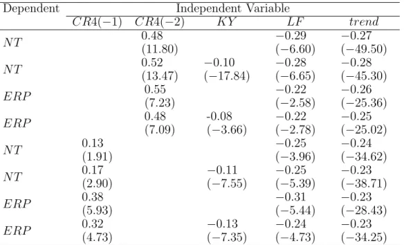
While the reduction of protection is a general phenomenon, the regime switch did not
affect all sectors to the the same extent. Consider for instance “automobiles, trucks and
buses” and “artificial textile fibers”. Between 1988 and 1990, the average tariff among the
41 sub-sectors for which we have good data fell by a quarter, while in the automobiles, trucks
and buses sub-sector it actually increased by 21 percent. As a result, the nominal tariff in
this sub-sector went from about one and a half times the mean tariff in 1988 to 2.4 times in
1993 and 1.7 times in 1994. On the other hand, the average tariff levied on artificial textile
fibers imports went from 1.4 the mean tariff in 1988 to less than 90% of the 1994 mean14.
Clearly, there are forces specific to the automobiles, trucks and buses industry partially
offsetting the general trend towards a reduction of protection in the Brazilian economy. At
the same time, those forces seem to be weaker in the textile industry.
Figure 2 presents the evolution of nominal tariffs and concentration in these two sectors,
normalized with respect to the median of manufacturing. Note that while concentration
in the automobiles, trucks and buses industry throughout the period is at least twice the
manufacturing median, the “artificial textile fibers” sector shows a below the median
con-centration level (fluctuating around 0.75). At the same time, while the average nominal
tariffs in both sectors were almost the same as in 1988 at about 1.5 times the median, in
1994 the average protection was twice the median in automobiles, trucks and buses and
13
The corresponding figures for the entire (56 sub-sectors) sample are 35.6 percent in 1988 and 10.07 percent in 1994.
14
0.00 0.50 1.00 1.50 2.00 2.50 3.00
88 89 90 91 92 93 94
cr4-Autom. tariff-Autom. cr4-Textiles tariff-Textiles
Figure 2: Protection and concentration
exactly the median in the textile industry.15 The poultry, the dairy and the vegetable oils
(bulk) industries, are other interesting examples of sectors in which concentration was above
(below) average in 1988, and trade protection did not fall as much as (fell more than) in the
remaining industries.
This evidence suggests that the model’s mechanism linking the maximum sustainable
tariff and industrial concentration might well have been at work in the case of Brazil, and
in the next section we formally test this hypothesis.
15
4
Model estimation
Our objective is to test the relationship derived in Section 2 between industry concentration
and trade protection. The theoretical discussion suggests that ceteris paribus, the higher the
concentration of a given industry, the higher the import tariffs applied on foreign imports.
Although the model we have discussed is strictly speaking static in nature, we can take
advantage of the panel structure of our dataset to analyze its performance in the trade
liberalization episode we are considering. In order to benefit from the time structure of our
dataset we initially used (one or two years) lagged CR4. Given that in the model causation
goes from concentration to tariff, we found it natural to use a predetermined concentration
index. Moreover, although the channel from industry structure to protection in the model is
same–period contributions, one can think that in practice there is a considerable time period
between the political decision of making a contribution and the final effect of obtaining a
given level of tariff.
We used the following equation in all estimations:
Tit =βi+φ.Zit+ǫit, i= 1, ...,21, t = 1988, ...,1994
where Tit is one of the two openness indicators for sector i at time t, Zit is a vector of
explanatory variables that always contains the concentration index and may or may not
contain additional control variables, βi is the industry-specific fixed effect, and ε is a zero
mean error term.
Our main data set consists of a panel of 21 industries for seven years (from 1988 to
1994). In all our regression we have used industry fixed effects. Introducing industry fixed
effects we can account for time invariant industry characteristics that are likely to have an
effect on concentration, like for instance large fixed setup costs, and that might otherwise
confound the interpretation of our results, making them for instance compatible with an
Table 2: N T regressions (fixed-effect method, lag concentration)
Model Independent Variable
CR4(−1) CR4(−2) KY trend
1 0.37
(3.35)
−0.23 (−29.43)
2 0.26
(2.95)
−0.10 (−2.29)
−0.21 (−27.50)
3 0.39
(4.29)
−0.23 (−29.22)
4 0.26
(3.60)
−0.09 (−2.97)
−0.20 (−27.52)
Note: t-statistic in parentheses; 21 cross-section observations
To statistically validate our choice, we also ran the Hausmann specification test to
de-cide between the fixed-effects and the random-effects method. With nominal tariffs as the
dependent variable, the result favored the fixed-effects method, which we therefore used in
all regressions. When the effective rate of protection was instead used, the results were
ambiguous depending on the control variables included in the regression and the time
pe-riod of the sample. We estimated our models using fixed effects also in this case. Table
2 presents the results for our first set of regressions. To avoid the potential endogeneity
problems which could arise using simultaneous concentration indicators16 we consider first
the results for nominal tariffs,N T and lagged concentration (all variables are in logs, except
for the trend).17
The results above support the hypothesis that industry concentration impacts nominal
tariffs, as the estimated coefficient of CR4 is positive and statistically significant at 5% in
all regressions. Moreover, the estimated impact is large: for a given capital-output ratio, a
16
We will discuss these later on in the paper. 17
difference of 20% in CR4 between industries implies 5% to 7% higher tariffs.
The inclusion of a time trend is meant to capture macroeconomic and policy changes
that affected the economy as a whole in the period. As already mentioned, there was a
generalized reduction in trade barriers for the manufacturing sector starting in 1988. In
our sample, the median tariff felt from 41.5% to 10.6%. But this decrease was not uniform
across industries, as tariffs of some sectors were in 1994 still two times above the median
tariff. The presence of the time trend in the regression simply excludes the common element
of this phenomenon. In fact, the estimated coefficient had the expected sign and was highly
significant in all regressions. The estimated result says that there was a 20% negative trend
in the nominal tariff value in the period18.
The results are robust to the inclusion of new controls. We tested different specifications
which included (various combinations of) capital intensity measures (KY), fixed capital
formation (IN V and M P), and profitability (J). The estimated coefficient of CR4 did not
change considerably and remained always significant. In table 2 we report the coefficients
for the capital output ratio, since this control has often been used in the literature. As in
Trefler (1993) the estimated impact is negative, and this might indicate that KY acts as
an entry barrier for both domestic and foreign competitors, so that it reduces the need for
protection and hence the observed tariff levels.19
Table 3 presents the outcome of the regressions in which we use our alternative measure
of protection (ERP). The results are similar to those for nominal tariffs, although the
18
Note that 20% annual reductions of the 1988 mean tariff (45.9%) for seven consecutive years almost matched the 1994 observed average tariff. The latter is 10.5% and the former 9.5%.
19
Table 3: ERP regressions (fixed-effect method, lag concentration)
Model Independent Variable
CR4(−1) CR4(−2) KY trend
1 0.43
(2.96)
−0.22 (−22.82)
2 0.33
(3.11)
−0.11 (−2.48)
−0.20 (−27.50)
3 0.48
(5.12)
−0.22 (−22.85)
4 0.21
(5.09)
−0.15 (−8.10)
−0.17 (−29.77)
Note: t-statistic in parentheses; 21 cross-section observations
estimated coefficients ofCR4 are in most cases larger. The estimated trend remained around
0.20 and KY is significant and negative in all models. As for nominal tariffs, we tested the
robustness of the model including different combinations ofIN V, M P, J in several regressions
and the estimated coefficient ofCR4, trend andKY did not change considerably and always
remained significant. The results in Table 3 are similar to the one obtained for nominal tariffs:
After controlling for a common trend, in those industries where concentration is higher, trade
protection is larger. According to our estimates, a 10% difference in concentration implies
a 2% to 5% difference in the effective rate of protection. A possible interpretation of these
results is that a given industry structure might well have an impact not only on the extent
of protection directly granted to its output, but also, through the value chain, to the extent
of protection granted to the intermediates required in the production process20.
We now turn to regressions with contemporary CR4. One important question to be
addressed in this context is that of the potential endogeneity of our measure of concentration.
One could well argue that the causation goes in a direction that is opposite to what we have
hypothesized in our model: Higher tariffs could produce less competition and consequently
20
Table 4: N T regressions (fixed-effects method)
Method Independent Variable
CR4 KY trend
OLS 0.13
(0.22)
−0.22 (−26.96)
OLS 0.19
(2.22)
−0.14 (−4.22)
−0.20 (−21.13)
2SLS −0.02
(−0.18)
−0.18
(26.94)
2SLS 0.27
(2.99)
−0.14 (−4.40)
−0.21 (−28.67)
Note: t-statistic in parentheses;J was the instrument in the two last equations. Variables are in logs.
higher concentration. If this were the case, our estimates would be biased and inconsistent.
To test this hypothesis, we ran a version of the Hausman test proposed by Davidson and
MacKinnon (1993) and used as an instrument the variableJ, which is reasonable to assume as
being correlated with CR4 but not withN T and ERP21. Again, the results are ambiguous.
For N T the test could not reject the hypothesis of consistent OLS estimates but for ERP,
depending on the time period, the test marginally rejected this hypothesis. To compare the
results, we will present in this case the OLS and (weighted) two-stage least square estimates
in Table 4.
Concentration has the same effect on trade policy as in Table 2, provided that we control
for capital intensity (KY): the estimated coefficient of concentration is once again
signifi-cant and positive, and the trend is found to be around 0.20 and barriers to entry (KY) also
appear to be significant. For this reason we cannot reject the hypothesis of current
con-centration affecting current trade policy. However, unlike in the case of past concon-centration,
21
Table 5: Extended data set (fixed-effect method)
Dependent Independent Variable
CR4(−1) CR4(−2) KY trend
N T 0(7.42.08) −(−045.25.53)
N T (50.28.21) (−−05.07.24) −(−045.23.30)
ERP 0(6.51.81) −(−031.24.52)
ERP 0(6.41.42) -0(−.083.68) −(−029.22.91)
N T 0(2.21.77) −(−042.22.61)
N T 0.18
(2.70)
−0.10 (−5.87)
−0.22 (−43.61)
ERP 0(4.35.18) −(−032.21.55)
ERP (40.30.05) (−−05.10.05) −(−034.20.76)
Note: t-statistic in parentheses; 41 cross-section observations
CR4 becomes insignificant if KY is removed from the model, and the same result holds
also when we introduce additional controls. One possible interpretation is that a model in
which concentration affects trade policy without delay does not find strong supported in the
data, as it has been found already in many other studies (Baldwin (1985), Goldberg and
Maggi (1999)). Results for the effective rate of protection are similar. Exploiting the time
dimension of our panel we are instead able to highlight how past concentration plays an
important role in determining current protection.
As a further robustness check, we have also estimated the specification discussed above
using the extended data set, which includes 41 industries. The main results are presented
in Table 5. The estimated elasticity of the N T or ERP with respect to our concentration
measures (CR4(−1) and CR4(−2)) as in the original data set, is always positive and
signifi-cant. Moreover, the point estimates for CR4(−2) are in general considerably higher than in
Table 6: Tariffs normalized by the annual median
Dependent Independent Variable
CR4(−1) CR4(−2)
M N T 0.41
(4.20)
M N T 0.49
(6.92)
M ERP 0.33
(2.08)
M ERP 0.46
(5.42)
Note: t-statistic in parentheses; 21 cross-section observations
another would have nominal tariffs 40% to 30% higher than the latter. The estimated trend,
as in all previous cases, is also around minus 20% a year in all regressions and entry barriers
seems to play a significant role. Once again, the link between industry concentration and
trade protection appears to be robust.
The relationship between industry structure and trade protection can also be tested by
regressing CR4 on tariffs normalized by the median (or mean) tariff of a given year. Using
this alternative strategy, we correct directly for the generalized reduction of nominal and
effective tariffs, without assuming a constant trend year to year. This is done in Table 6,
where M T N is the nominal tariff divided by the median of the corresponding year and
M ERP is ERP divided by the median.
We used the (weighted) fixed-effect method in all regressions. The results above are
evidence that the higher the seller concentration in a given industry, the greater the distance
of its tariffs to the median tariff (with elasticities between one third and 50%). Moreover,
the use of a constant trend did not affect the estimated coefficients of the concentration
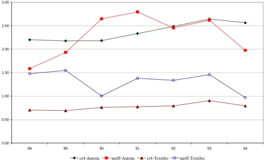
Table 7: Extended data set (fixed-effect method)
Dependent Independent Variable
CR4(−1) CR4(−2) KY LF trend
N T (110.48.80) (−−06.29.60) −(−049.27.50)
N T (130.52.47) −(−017.10.84) −(−06.28.65) −(−045.28.30)
ERP (70.55.23) (−−02.22.58) −(−025.26.36)
ERP (70.48.09) -0(−.083.66) −(−02.22.78) −(−025.25.02)
N T (10.13.91) (−−03.25.96) −(−034.24.62)
N T 0.17
(2.90)
−0.11 (−7.55)
−0.25 (−5.39)
−0.23 (−38.71)
ERP (50.38.93) (−−05.31.44) −(−028.23.43)
ERP (40.32.73) −(−07.13.35) −(−04.24.73) −(−034.23.25)
Note: t-statistic in parentheses; 41 cross-section observations
results are robust to the inclusion of the additional controls available in our dataset.22
To further evaluate the robustness of our results, we run a last group of regressions
controlling for industry size. It is common in the literature (e.g., Caves (1976)) to argue
that protection should be positively related to the number of employees of a given industry,
as this might result in more votes being delivered to politicians deciding on trade measures.
In Table 5 we present regressions with the extended database in which we use “total labor
force employed in production” (LF), to capture the role of industry size. Also when we
account for the role of industry size, our estimates suggest that past concentration continues
to play an important role in predicting protection. Controlling for employment does not
alter the main results and the magnitudes of the estimated coefficients are close to those in
Table 5.
22
5
Conclusions
The recent Brazilian trade liberalization episode is a natural experiment to evaluate the
importance of industry structure as a determinant of tariff protection. In the past, a large
body of literature has focused overwhelmingly on the United States to examine the problem
in a cross sectional setup, and has failed to identify a robust relationship between tariff
protection and industrial concentration. In this paper we have instead taken advantage of
the major policy shift implemented in Brazil in the early nineties to re-evaluate the problem
using a panel data set covering the manufacturing sector. The inclusion of a time dimension
in the data has allowed us to avoid some of the obvious endogeneity problems, and we have
shown that industrial concentration is an important determinant of protection. Our results
are robust to the various alternative specifications we have considered, and we hope that this
might inspire additional work on trade policy and industrial structure, in which the time
dimension is appropriately taken into account.
References
Baldwin, R. (1985). The Political Economy of US import policy. Cambridge, MA: MIT
Press.
Caves, R. (1976). Economic models of political choice: Canada’s tariff structure.Canadian
Journal of Economics 9, 278–300.
Ferreira, P. C. and J. L. Rossi (2003). New evidence from brazil on trade liberalization
and productivity growth.International Economic Review forthcoming.
Gawande, K., P. Sanguinetti, and A. K. Bohara (2003). Trade diversion and declining
tariffs: Evidence from mercosur.Journal of International Economics. forthcoming.
Geraldino da Silva, G. (1999). Estrutura de mercado e desempenho: Evidˆencias emp´ıricas
Goldberg, P. K. and G. Maggi (1999). Protection for sale: An empirical investigation.
American Economic Review 89(5), 1135–55.
Grossman, G. M. and E. Helpman (1994). Protection for sale. American Economic
Re-view 84, 833–850.
Hay, D. A. (2001). The post-1990 Brazilian trade liberalization and the performance of
large manufactuiring firms: Productivity, market share and profits. Economic
Jour-nal 111, 620–641.
Helfand, S. M. (2000). Interest groups nad economic policy: Explaining the pattern of
protection in the Brazilian agricultural sector. Contemporary Economic Policy 18,
462–476.
Kume, H. (1996). A pol´ıtica de importa¸c˜ao no plano real e a estrutura de prote¸c˜ao efetiva.
Texto para Discuss˜ao 423, IPEA.
Magee, C. (2002). Endogenous trade policy and lobby formation.Journal of International
Economics 57, 449–471.
Maggi, G. and A. Rodriguez-Clare (1998). The value of trade agreements in presence of
political pressure. Journal of Politcal Economy 106, 574–601.
Mitra, D. (1999). Endogenous lobby formation and endogenous protection: A long-run
model of trade policy determination. American Economic Review 89(5), 1116–34.
Muendler, M.-A. (2002). Trade, technology and productivity: A study of Brazilian
man-ufacturers, 1986-1998. mimeo, University of California, Berkeley.
Olarreaga, M. and I. Soloaga (1998). Endogenous tarif formation: The case of Mercosur.
World Bank Economic Review 12, 297–320.
Olson, M. (1965). The Logic of Collective Action. Harvard University Press.
Pecorino, P. (1998). Is there a free-rider problem in lobbying? Endogenous tariffs, trigger
Rodrik, D. (1986). Tariffs, subsidies and welfare with endogenous policy. Journal of
In-ternational Economics 21, 285–299.
Rodrik, D. (1995). Political Economy of trade policy. In G. M. Grossman and K. Rogoff
(Eds.), Handbook of International Economics, Volume 3, pp. 1457–1494. Amsterdam
and New York: North Holland.
Trefler, D. (1993). Trade liberalization and the theory of endogenous protection: an
! " # $% & '( ))* # + ,-".
* / 0123 4 1 / 0 5 0 6 1
0 4 / / (. %( '( 7 (% 4(.. 5( ' /( . #
$% & '( ))* # 8 ,-".
23 9 0 23 5 2 0 (. ' .
' . . $% : ( (;(. 5 & 4(' 5( ( # $% & '( ))* # *
,-".
8 < = 4 1 > 0 / 9 ?@@A )) ' : (.
0 % ( 5( ' '( < ' 7 . $% & '( ))* # ?A ,-".
A 5 0 B 1 0 > 0 B 0 $ "(
(. 0( ' & %; # $% & '( ))* # ,-".
+ 1 10 0B 4 1 10 5 0 6
440 > 0 C1 B /( " 0( ' & %; # $% &
'( ))* # A ,-".
1 5 < 4 0 B 1 51 5 < 0 4
# ( 5( '(. # $% & '( ))* # ?) ,-".
@ / D 5 0 B 5 55 40
0( ' %; $( ( E & ( ' %; # $% & '( ))* # ) ,-".
@) 9 4 50 23 F 4 5 G
( ( H " ( (. # $% & '( ))* # 8 ,-".
@? 5 0 B 0 6 0B 5 < ))? 4
> 0 0( ' & %; 0 $ "( (. # $% & '( ))* # + ,-".
@ < 0 =6 1 < 1
0 5 / B $ I / .. ( 5 .& '
/ & ' # " . '( ))* # A ,-".
@* 0 D < 0 . ( 5 ('( . (
( / ' (. # " . '( ))* # A ,-".
@ 0 B 5 1 1 H 4 0 0 6 4 0
44 < %( '( 7 (% 4(.. . 4(.. J ( 7 # " . '( ))*
# *) ,-".
@8 D4 G F0 )
# %( '( 7 (% 4(.. # " . '( ))* # ,-".
@A 0 B 1 1 B # . %"K ' . # ( ( 7 '( ))* # )
,-".
@+ = < < < 1 < 0 00 / 0 . %"K ' . #
@ 1 H < 1 / L D L < . %"K ' . # ( ( 7 '( ))* # *) ,-".
@@ 4 0 D H < 1 0 0 5 B4 . %"K ' . #
( ( 7 '( ))* # A ,-".
8)) / 0 4 C1 4 0 4
2M $ I / .. ( &( % 5( ( # ( ( 7 '(
))* # @ ,-".
8)? 5 0B 5 1 / 0 1 0 ( 5( '(.
$ & " # ( ( 7 '( ))* # *+ ,-".
8) 4 4 5 5 0 1 0
( 5( '(. $ & " # ( ( 7 '( ))* # ,-".
8)* < ! N0 B
O # 0( ' & %; # ( ( 7 '( ))* # ??,-".
8) < 5 < C1 < 0 H / 0 =&
# ( ( 7 '( ))* # * ,-".
8)8 1 4 10 < 5 50 H <
4 5 0 B . / '( & # % %7 '( ))* #
+ ,-".
8)A 4 6 40 1 1 1 P . < /
QR ( 5 S (. $ # % %7 '( ))* # ,-".
8)+ 4 1 51 1 4 0 H < 1 4('
5( ( $ I / .. ( %( '( 7 (% 4(.. # % %7 '( ))* #
,-".
8) < 10 1 0 4 0 / P ( (7 <% 7( ( #
% %7 '( ))* # 8 ,-".
8)@ 4 < 1 10 5 (
5 S (. $ # % %7 '( ))* # ** ,-".
8?) 1 41 / 1 6 10 / /
( ( 5 S (. $ ( T # % %7 '( ))* # *A ,-".
8?? 1 00 0 T. QR $ .: 5 R ' 7 & 4-. #
( 7 '( ))* # *+ ,-".
8? 1 < 4 0 C1
T. %R <% 7( ( # ( 7 '( ))* # *? ,-".
8?* C1 0 1 B = H < 11 5 %R / 5
. ' & 4 = ( # ( 7 '( ))* # ?+ ,-"!.
8? 4 10 / = 4 1 1 B 6 H 05
8?8 0 > U V6 (
5 S (. $ # ( 7 '( ))* # + ,-".
8?A / / 1 6 1 (
5 S (. $ # ( 7 '( ))* # + ,-".
8?+ / 0 4 2 / 5( ' '( < '
7 . # (;( 7 '( ))* # ?+ ,-".
8? 4 9 W ( S (. :
5 7 ' (;( 7 '( ))* # * ,-".
8?@ < 1 ( S (. : ( D( (;
(;( 7 '( ))* # ,-".
8 ) H 0B 5 > 0 0 4 0 1 10 40
1 ( S (. : (;( 7 '( ))* # 88 ,-".
8 ? < 1 < 0 44 < < H 05 5 50 %7( .
4( & E. ( # $ ( '( )) # ?A ,-".
8 0 0 < 5 B = 0 51 0 (
5( '(. 4 % = "( ( # 5( ( ( '( )) # * ,-".
8 * < 55 H / 1 = T. %R
<% 7( ( . < .% & ' # 5( ( ( '( )) # ? ,-".
8 / 0 P T. %R <% 7( ( . <
.% & ' # 5( ( ( '( )) # A ,-".
8 8 .(' "( .9 " ; '(. " 9 ' ( ( , . . . (
5( ( <% 7( ( # 5( ( ( '( )) # ?? ,-".
8 A 0 ' X(. 0 ( (X $% $ ..% YI <% 7( ( #
5( ( ( '( )) ?@ ,-".
8 + ' ' (. '( (. '( ' '( ( S ( % " '( ( (..Z(. ,
. "( $ ! ( ( % ( $ I / .. ( ' ( , 5( ( ( '(
)) # ? ,-".
8 1 4 00B 4 / >& R ( D 0% ;
( 0 # Y '( )) # + ,-".
8 @ < = 4 0B < 1 41 P 0 0 4 B
0% ; ( 0 >& R ( D # Y '( )) # ? ,-".
8*) H 4 4 / < 444 <B4 < E % " = 0% ; ( 0 # Y
'( )) # *A ,-".
8*? 0 0 > 1 0 6 / 5 > 0