www.atmos-chem-phys.net/12/5413/2012/ doi:10.5194/acp-12-5413-2012
© Author(s) 2012. CC Attribution 3.0 License.
Chemistry
and Physics
Transport of mesospheric H
2
O during and after the stratospheric
sudden warming of January 2010: observation and simulation
C. Straub1, B. Tschanz1, K. Hocke1,2, N. K¨ampfer1,2, and A. K. Smith3
1Institute of Applied Physics, University of Bern, Switzerland
2Oeschger Center for Climate Change Research, University of Bern, Switzerland
3Atmospheric Chemistry Division, National Center for Atmospheric Research, Boulder CO, USA
Correspondence to:C. Straub ([email protected])
Received: 20 October 2011 – Published in Atmos. Chem. Phys. Discuss.: 12 December 2011 Revised: 12 May 2012 – Accepted: 4 June 2012 – Published: 22 June 2012
Abstract. The transportable ground based microwave ra-diometer MIAWARA-C monitored the upper stratospheric and lower mesospheric (USLM) water vapor distribution over Sodankyl¨a, Finland (67.4◦N, 26.6◦E) from January to June 2010. At the end of January, approximately 2 weeks after MIAWARA-C’s start of operation in Finland, a strato-spheric sudden warming (SSW) disturbed the circulation of the middle atmosphere. Shortly after the onset of the SSW water vapor rapidly increased at pressures between 1 and 0.01 hPa. Backward trajectory calculations show that this strong increase is due to the breakdown of the polar vor-tex and meridional advection of subtropical air to the Arc-tic USLM region. In addition, mesospheric upwelling in the course of the SSW led to an increase in observed water vapor between 0.1 and 0.03 hPa.
After the SSW MIAWARA-C observed a decrease in mesospheric water vapor volume mixing ratio (VMR) due to the subsidence of H2O poor air masses in the polar
re-gion. Backward trajectory analysis and the zonal mean wa-ter vapor distribution from the Microwave Limb Sounder on the Aura satellite (Aura/MLS) indicate the occurrence of two regimes of circulation from 50◦N to the North Pole: (1) regime of enhanced meridional mixing throughout Febru-ary and (2) regime of an eastward circulation in the USLM region reestablished between early March and the equinox. The polar descent rate determined from MIAWARA-C’s 5.2 parts per million volume (ppmv) isopleth is 350±40 m d−1
in the pressure range 0.6 to 0.06 hPa between early Febru-ary and early March. For the same time interval the de-scent rate in the same pressure range was determined using Transformed Eulerian Mean (TEM) wind fields simulated by
means of the Whole Atmosphere Community Climate Model with Specified Dynamics (SD-WACCM). The average value of the SD-WACCM TEM vertical wind is 325 m d−1while the along trajectory vertical displacement is 335 m d−1. The similar descent rates found indicate good agreement between the model and MIAWARA-C’s measurements.
1 Introduction
Water vapor enters the stratosphere from the equatorial tro-posphere through the tropical tropopause layer from where it is transported upward into the mesosphere following the Brewer-Dobson circulation (Andrews et al., 1987). As the tropical tropopause layer acts as a cold trap the whole mid-dle atmosphere is extremely dry (Brewer, 1949). The positive vertical gradient throughout the stratosphere is due to the sec-ond source of H2O in the middle atmosphere, the oxidation
of methane while the negative vertical gradient in the meso-sphere is mainly caused by photo-dissociation due to the ab-sorption of solar Lymanαradiation (Brasseur and Solomon, 2005).
The chemical lifetime of water vapor is in the order of months in the lower mesosphere and in the order of weeks in the upper mesosphere (Brasseur and Solomon, 2005). This is long with respect to dynamical processes and water vapor is therefore a tracer for atmospheric transport. The zonal mean distribution of water vapor in December 2009 as measured by Aura/MLS (Waters et al., 2006) is displayed in Fig. 1. As the vertical H2O gradient is negative throughout the
Fig. 1.Zonal mean distribution of middle atmospheric water vapor as measured by EOS/MLS through December 2009. Red indicates relatively higher values and blue relatively lower values.
investigate polar winter descent and humid air from around the stratopause for polar summer ascent. The polar winter de-scent induces horizontal gradients in the H2O volume
mix-ing ratio (VMR) as the mesospheric air descendmix-ing within the polar region is much dryer than the air outside of it. Due to this horizontal gradient water vapor is a valuable tracer for short term mixing in the winter hemisphere, e.g. in the course of stratospheric sudden warmings. Around the stratopause H2O is not a good tracer due to its local maximum in the
upper stratosphere (Lee et al., 2011).
Stratospheric sudden warmings (SSW) are extreme events in the middle atmosphere characterized by a fast and strong increase of stratospheric temperature (usually at least 25 K in a week or less) and simultaneous cooling of the meso-sphere. The main cause for SSWs are planetary waves ex-cited in the troposphere propagating up into the stratosphere where they interact with the mean flow (Matsuno, 1971; Liu and Roble, 2002). Dissipation of planetary waves decelerates the polar night jet and induces a pole ward residual circula-tion, which produces adiabatic heating due to downward flow in the high latitude stratosphere and adiabatic cooling due to upward flow in the high latitude mesosphere. The forcing by planetary waves can be strong enough to reverse the polar night jet.
In the course of SSWs the stratospheric polar vortex is strongly distorted and either shifted off the pole (vortex dis-placement event) or even split in two pieces (vortex split event), (Charlton and Polvani, 2006). There has been a strong vortex displacement event in 2006 and a strong vortex split event in 2009. Both SSWs were used to thoroughly study dy-namics and transport processes during SSWs (e.g. Coy et al., 2009; Harada et al., 2010; Siskind et al., 2010; Funke et al., 2010). The weakening of the high-latitude transport barrier in the course of a SSW can lead to strong mixing of air masses.
Manney et al. (2008, 2009a,b) investigated transport of the trace gases CO, H2O and N2O during the warmings in 2006
and in 2009 using satellite data from Aura/MLS, ACE/FTS and TIMED/SABER and model outputs from SLIMCAT, GEOS5 and ECMWF. These trace gases showed values char-acteristic of low and mid-latitudes extending to Polar Re-gions and extremely weak gradients throughout the hemi-sphere. Approximately 3 weeks after both the 2006 and 2009 SSWs, the vortex in the upper stratosphere and lower meso-sphere (USLM) reformed, reestablishing the mixing barri-ers and strong diabatic descent developed, echoing the pat-tern of descent typically seen in fall, see e.g. Siskind et al. (2007), Orsolini et al. (2010), Smith et al. (2011) and refer-ences therein.
The fall and winter descent in the USLM vortex can be regarded as a part of the mesospheric branch of the Brewer-Dobson circulation (Brewer, 1949). The determination of the velocity of polar winter descent is of scientific interest as it provides important information for the characterization of the meridional circulation.
Fall descent rates for the upper stratosphere in both hemi-spheres have been modeled by Manney et al. (1994) who ob-tained a value of approximately 260 m d−1for the 1992/1993 Arctic vortex. In addition there have been studies investi-gating the descent rate in the Arctic/Antarctic middle atmo-sphere using ground based measurements. Forkman et al. (2005) determined fall descent rates of up to 300 m d−1 at 75 km altitude at 60◦N using CO and H2O data while Allen
et al. (2000) found Antarctic fall descent rates of 250 m d−1 at 60◦S and 330 m d−1at 80◦S in the upper stratosphere
us-ing CO data.
There have only been few studies investigating USLM de-scent rates after SSWs. Using observations of Aura/MLS and Empirical Orthogonal Function analysis Lee et al. (2011) determined descent rates of approximately 1500 m d−1 at 80 km decreasing linearly to 500 m d−1 at 60 km for the time after the 2006 and 2009 SSWs. Salmi et al. (2011) found mesosphere to stratosphere descent rates of approxi-mately 700 m d−1after the 2009 SSW using NOxdata from
ACE/FTS and the FinROSE chemical transport model. After the SSW of February 2004 Nassar et al. (2005) estimated a descent rate of 150 m d−1in the upper stratosphere from CH4
and H2O measurements of ACE/FTS.
was associated with meridional transport while the observed ozone depletion was mainly due to temperature-dependent photochemistry in the upper stratosphere (above 5 hPa) and mainly due to transport of polar air to mid-latitudes in the lower stratosphere (below 5 hPa). de Wachter et al. (2011) observed a decrease in mesospheric water vapor over Seoul, South Korea, during the SSW 2008 which they attributed to polar air being transported to such low latitudes when the polar vortex was shifted towards Europe in the course of the SSW.
In this paper we investigate horizontal transport through-out the mesosphere during and after the SSW 2010 using backward trajectory calculations at several mesospheric al-titudes. In addition we present post SSW Arctic mesospheric descent rates determined from ground based and space borne water vapor measurements and TEM vertical wind and tra-jectory calculations. To our knowledge this is the first study investigating polar descent after a SSW using ground based data.
The article is organized as follows. Sections 2 and 3 present the measured and modeled data sets used. Section 4 introduces the trajectory computations. Section 5 gives an overview about dynamical changes during the SSW of Jan-uary 2010. Section 6 presents the measured water vapor dis-tribution and discusses influences of the SSW upon it. Sec-tion 7 shows conclusions drawn from this study.
2 Measurement data
Water vapor data from two sources, a ground based and a space borne microwave radiometer, are used in this study.
2.1 Ground based microwave radiometer MIAWARA-C
The first source is measurements of the vertical distribution of H2O VMR over Sodankyl¨a, Finland (67.4◦N, 26.6◦E)
recorded by the ground based MIddle Atmospheric WAter vapor RAdiometer MIAWARA-C belonging to the Univer-sity of Bern, Switzerland. The instrument has been oper-ated at the Finnish Meteorological Institute Arctic Research Center from mid-January to mid-June in the frame of the Lapland Atmosphere-Biosphere Facility (LAPBIAT2) cam-paign. MIAWARA-C has been specifically designed for mea-surement campaigns. The instrument has two main functions; it serves as a traveling standard for inter-comparison (Straub et al., 2011; Leblanc et al., 2011; Stiller et al., 2012) and it is used in measurement campaigns focusing on dynamic processes. The instrument is of a compact design and has a simple set up procedure. It can be operated as a standalone instrument as it maintains its own weather station and a cal-ibration scheme that does not rely on other instruments nor the use of liquid nitrogen. Water vapor profiles are retrieved from measured spectra of the pressure broadened 22 GHz
rotational emission line (see Straub et al., 2010, 2011 for details on MIAWARA-C). Here, data from 10 January to 31 March 2010 is considered and analyzed to yield daily es-timates of water vapor profiles in an altitude range between 10 and 0.02 hPa (approximately 30 to 75 km) with a verti-cal resolution of approximately 12 km. The uncertainty on MIAWARA-C’s profiles is typical for ground based 22-GHz water vapor radiometers as shown in Straub et al. (2010, 2011). The simulated accuracy (determined as the 2-σ sys-tematic error arising from uncertainties in a priori temper-ature, in calibration and in spectroscopy) is below 16 % at all altitudes, while the simulated precision (determined by propagation of 1-σ measurement noise) degrades from 5 % at altitudes up to 50 km to 18 % between 50 and 75 km.
2.2 Aura/MLS
The second source of data is the Microwave Limb Sounder (MLS) aboard the Aura satellite described in Waters et al. (2006). Daily zonal averages of H2O VMR and temperature
MLS acquired in the northern hemisphere over the time in-terval 10 January to 31 March 2010 are considered here. The highest latitude accessible to the satellite is 82.5◦N. MLS yields water vapor as one of its version 2.2 level 2 data products covering the pressure range of 316 to 0.002 hPa. The vertical resolution of this retrieval version is 3–4 km in the stratosphere but degrades to approximately 12 km at 0.1 hPa and above. The single profile precision (1-σ random error estimated from the level 2 algorithms) is 4–9 % in the stratosphere and degrades from 6 to 34 % between 0.1 and 0.01 hPa. The accuracy (likely magnitude of 2-σ systematic error) is estimated to be 4 to 11 % for the pressure range 68 to 0.01 hPa (Lambert et al., 2007). The Aura satellite is in a Sun-synchronous orbit passing through two local times at any given latitude. For this analysis zonal mean water va-por at 67◦N is used in order to complement MIAWARA-C’s point measurements with zonal mean profiles. When using mean values of a number of profilesnit is assumed that the systematic bias (accuracy) is the same as for a single pro-file while the 1-σ random uncertainty decreases by a factor 1/√n.
3 Model data 3.1 ECMWF
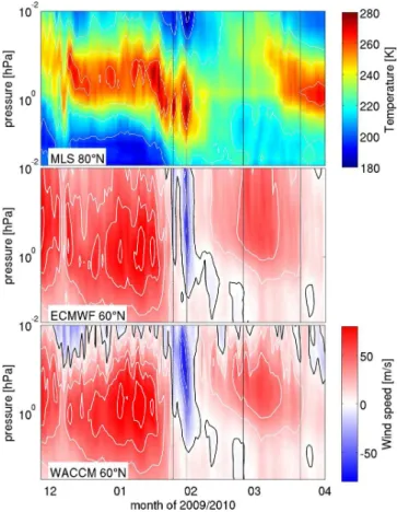
Fig. 2.MLS zonal mean temperature at 80◦N and ECMWF and SD-WACCM zonal mean zonal wind at 60◦N. Top panel: red rela-tively higher values and blue relarela-tively lower values. Middle panel: red eastward winds and blue westward winds from ECMWF. Bot-tom panel: red eastward winds and blue westward winds from SD-WACCM. The vertical lines indicate the following dates (from the left): 24 January (wind reversal mesosphere), 30 January (maximum temperature at 60◦N and 10 hPa), 24 February (end of the time of enhanced meridional mixing) and 21 March (equinox).
in longitude. On 26 January 2010 ECMWF’s operational data set was update from version T799 to T1279 (ECMWF, 2012b), i.e. the horizontal resolution has been increased from 25 to 16 km. However, before any new operational imple-mentation, the old and new versions are run side by side. In order to avoid discontinuity in the analyzed data T1279 is used during the whole time.
The mesospheric levels of ECMWF are relatively close to the model top. However, the model still maintains a good representation of gravity wave drag processes and it produces a relatively realistic Brewer-Dobson circulation as shown by Monge-Sanz et al. (2007).
3.2 SD-WACCM
This study presents results from the NCAR Whole Atmo-sphere Community Climate Model with Specified Dynam-ics (SD-WACCM). WACCM uses a free-running
dynami-Fig. 3.This figure follows loosely the style of Fig. 1 in Manney et al. (2009b).(a)MLS zonal mean temperature as function of time and pressure at 60◦N in 2010 (red relatively higher values, blue relatively lower values),(b)MLS temperature,(c)ECMWF zonal wind,(d) altitude wave 1 from ECMWF and(e)altitude wave 2 from ECMWF. The red curves indicate temperature, zonal mean zonal wind, wave 1 and wave 2 for 2010 while the blue curve in-dicates corresponding values for the 2009 SSW which occurred at the almost same time of the year (major SSW criterion was fulfilled on 24 January). For details see text. The vertical lines indicate the following dates (from the left): 24 January (wind reversal meso-sphere), 30 January (maximum temperature at 60◦N and 10 hPa), 24 February (end of the time of enhanced meridional mixing) and 21 March (equinox).
The gravity wave parameterization in WACCM (Richter et al., 2010) determines the mean flow forcing from a discrete spectrum of gravity waves that are forced interactively in the troposphere by topography, convection (mostly in low lati-tudes), and frontal dynamics (middle and high latitudes). The parameterization also gives a coefficient for vertical eddy dif-fusion that affects heat and the mixing ratios of trace species. In the current study, SD-WACCM is nudged with 1 % of the GEOS-5 meteorological fields (e.g. temperature, zonal and meridional winds, and surface pressure) every 30 min. The nudging alters the model predictions by effectively com-bining 0.99×the model predicted field with 0.01×the value from the assimilation model, i.e.,T =0.99×T (WACCM)+
0.01×T(GEOS-5). It is applied below 50 km and tapers to zero between 50 and 60 km. The GEOS-5 analysis is avail-able with a time resolution of 6 h and is interpolated to the 30-min nudging intervals. Latitude and longitude resolution for these WACCM runs is 1.9×2.5◦and there are 88 pres-sure levels from the surface to 150 km altitude. The nudg-ing allows SD-WACCM to perform as a chemical transport model in the troposphere and stratosphere. The model gener-ates mesospheric dynamical fields, in effect performing as a free-running model above 60 km except that the forcing from below is based on observations.
3.3 Mesospheric wind in the two models
Lower mesospheric winds are poorly observed and therefore models with assimilated data are probably our best way of determining 4 dimensional wind fields at these altitudes. The two models used in this study, ECMWF and SD-WACCM, assimilate data or are nudged with assimilated data, respec-tively, in the lower and middle stratosphere and are uncon-strained in the upper levels. Therefore, the inaccuracy of their wind fields increases with altitude in the mesosphere. How-ever, Liu et al. (2008) show that in WACCM error growth is limited when the lower atmosphere is continually reini-tialized, as it effectively is in the SD-WACCM. In addition WACCM includes a physically based gravity wave source parameterization which realistically simulates zonal mean winds (Richter et al., 2010). Still, the mesospheric winds of ECMWF and SD-WACCM suffer under large uncertainties and need to be handled with care. A comparison between the zonal mean zonal winds from the two models is given in the middle and lower panels of Fig. 2 (the discussion of this fig-ure, which in addition shows MLS zonal mean temperature in the top panel, follows in Sect. 5). The plots illustrate that below 0.1 hPa there is a good qualitative agreement between the two data sets while there are major differences even in the wind directions above that level. At altitudes above 0.1 hPa the zonal mean winds of SD-WACCM are regarded as more reliable than those of ECMWF since the upper model bound-ary of WACCM (approximately 150 km) is higher than the one of ECMWF (approximately 80 km). Therefore, WACCM outputs are used to illustrate zonal mean winds at these
alti-tudes. ECMWF data and Lagrangian backward trajectories are only presented up to 0.1 hPa.
4 Data analysis
This paper presents two different trajectory computation methods with two different information contents: (1) La-grangian backward trajectories started over Sodankyl¨a giving information on horizontal (zonal and meridional) and vertical origin of air parcels sampled by MIAWARA-C and (2) zonal mean trajectories started at 67◦N following the transformed Eulerian mean (TEM) circulation giving information on large scale meridional and vertical advection of air masses due to the combined effects of zonally averaged winds and wave momentum transport.
In general the TEM trajectories are regarded as more reli-able than the Lagrangian trajectories especially in the meso-sphere. The reason is that zonal mean winds are used for the calculation of the TEM trajectories while for the calculation of the Lagrangian trajectories 4 dimensional wind fields are needed. Nezlin et al. (2009) point out that scales smaller than total horizontal wavenumber 10 are not well represented in the mesosphere by any data assimilation system. As the La-grangian trajectories are calculated on scales much smaller than wavenumber 10 this introduces a large uncertainty.
However, the authors understand that additional informa-tion about mixing processes can be gained from the La-grangian trajectories despite their large uncertainties.
4.1 Lagrangian backward trajectories
The Lagrangian backward trajectories are computed using the LAGRangian ANalysis TOol LAGRANTO described in Wernli and Davies (1997) together with the wind fields pro-vided by ECMWF operational data (ECMWF, 2012a).
Daily 3-day backward trajectories are calculated for every USLM pressure level of MIAWARA-C’s retrieval grid below 0.1 hPa. As the photo-chemical lifetime of H2O is in the
or-der of months in the lower mesosphere and weeks in the up-per mesosphere, its VMR is assumed to be conserved along the trajectory. The trajectories give the geographical origin of the air masses measured by MIAWARA-C.
As there is no observational information on upper strato-spheric and mesostrato-spheric water vapor in the ECMWF system the water vapor values along the trajectories are determined from MLS observations. For each trajectory point (each alti-tude and day) the MLS profiles within±1◦in latitude,±10◦ in longitude and±0.5 d in time are searched. This search re-sults in one or two profiles per trajectory point. The H2O
4.2 TEM backward trajectories
The TEM circulation describes the bulk motion of large scale air masses as it closely approximates the net air par-cel displacement in the latitude-pressure plane (Andrews and McIntyre, 1976). The TEM trajectories are calculated us-ing daily TEM velocities determined from daily averaged WACCM model output. The approach used for the trajec-tory computations is the same as in Smith et al. (2011). For the analysis presented in this paper the daily backward tra-jectories are started at 67◦N for every USLM pressure level of MIAWARA-C’s retrieval grid. For the illustration of short term vertical motion 3-day backward trajectory calculations are shown and 20-day backward TEM trajectories are pre-sented in order to illustrate the residual meridional circula-tion (Brewer-Dobson circulacircula-tion).
5 The SSW 2010
5.1 Dynamical overview
The temperature and wind evolution of the 2010 SSW was similar to the major SSW of late January 2009 described in Manney et al. (2009b). The polar stratopause dropped and broke down (nearly isothermal middle atmosphere) and then reformed at a high altitude (∼0.03 hPa). As this effect is most pronounced at latitudes north of 70◦N the temperature evolution at 80◦N is displayed in the upper panel of Fig. 2. The lower panel shows the temporal evolution of ECMWF zonal mean zonal wind at the approximate latitude of the polar night jet (60◦N). In December and January the polar night jet is visible as an eastward circulation centered around 60◦N and 1 hPa. By the end of January the wind rapidly decelerates, the polar vortex shifts towards Europe and the zonal mean temperature at 10 hPa and 60◦N increases by approximately 25 K with the maximum on 30 January (sec-ond vertical line in the figures). The zonal mean latitudinal temperature gradient is positive in that time. The zonal mean wind reverses at altitudes above 10 hPa and latitudes north of 60◦N on 24 January (first vertical line in the figures) with maximum westward wind speeds of 60 m s−1at 0.3 hPa and 65◦N on 29 January. After the 2010 SSW the zonal wind in the stratosphere stays weak and the polar vortex does not re-cover at its original latitude before the circulation reverses to summer easterlies in the end of March (Fig. 2). In the meso-sphere an eastward circulation returns approximately 10 days after the wind reversal and by the end of February a USLM vortex forms reestablishing a weak mixing barrier. This is similar to the evolution observed after the SSW 2009 (Man-ney et al., 2009b) except that in 2010 the post SSW USLM vortex remained weaker than in 2009.
In order to point out similarities and differences a direct comparison between the SSW of January 2010 (red line) and the SSW of January 2009 (blue line) is given in
pan-els b, c, d and e of Fig. 3. As the two warmings occurred at a similar time of the year (in 2009 the major SSW cri-terion was fulfilled on 24 January) the same axis showing month of 2008/2009 or 2009/2010, respectively is used for both lines. This figure is loosely based on Fig. 1 in Man-ney et al. (2009b) comparing the SSWs of 2006 and 2009. In January 2009 the anomalous increase in stratospheric tem-perature was faster and slightly stronger than in 2010. The same is true for the deceleration of the zonal mean zonal wind at 60◦N and 10 hPa. In 2009 the zonal wind reversal was accompanied by strong geopotential height wave 2 am-plification (vortex split event) while geopotential height wave 1 was strong in December but weakened in the beginning of January. A few days after the maximum temperature slight wave 1 amplification was evident. In the beginning of win-ter 2009/2010 geopotential height wave 1 was weaker than at the same time of the previous year but it amplified before the SSW in January at the same time as the zonal mean zonal wind decelerated. This indicates that the January 2010 SSW was a vortex displacement event. The amplitude of wave 2 had a peak in mid-December when a minor SSW occurred but stayed fairly weak for the rest of the winter.
5.2 Zonal mean water vapor distribution indicating horizontal mixing and vertical motion
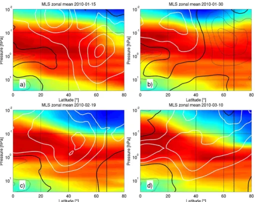
An overview of the northern hemisphere water vapor zonal mean distribution as observed by MLS before, during and af-ter the SSW 2010 is shown in Fig. 4 together with WACCM zonal mean zonal wind. On 15 January, before the SSW, the mixing barrier given by the polar night jet is clearly visible in the form of a maximum in eastward wind at 60◦N and 1 hPa and a strong horizontal gradient in mesospheric water vapor VMR with dry air north of 60◦ N and humid air south of it (panel a). During the SSW, on 30 January, the day of the maximum warming/cooling in the stratosphere/mesosphere, the situation has reversed: now the middle atmospheric zonal wind in the Arctic has changed to westward and the meso-sphere (at altitudes above 0.1 hPa) is more humid north of 60◦N than south of it (panel b). This situation is short lived and only persists for 3 days. It is linked with the strong meso-spheric upwelling in the course of the SSW leading to the observed cooling above 0.1 hPa.
For approximately three weeks after the warming the mean horizontal water vapor distribution in the mesosphere at lat-itudes between 45 and 82.5◦N is close to uniform and the maximum in zonal mean eastward wind is situated at approx-imately 40◦N in the mesosphere (panel c shows 19 Febru-ary as an example). The disappearance of meridional H2O
gradients indicates strong horizontal mixing between mid-latitudes and the Arctic. Approximately four weeks after the SSW the horizontal H2O gradient at around 60◦N has
Fig. 4.Evolution of MLS zonal mean H2O VMR (colors, red relatively higher values, blue relatively lower values) and WACCM zonal mean zonal wind (contours, contour interval=20 m s−1, bold black=0, white=eastward, black=westward) during the 2010 SSW.(a)before the SSW (15 January),(b)during the SSW (30 January),(c)during the time of enhanced mixing (19 February) and(d)when the USLM vortex has reestablished (10 March). The black dashed vertical line marks the latitude of Sodankyl¨a.
that the polar vortex did not recover to its original strength. The mid-latitude mesosphere especially at altitudes between 0.1 and 0.03 hPa is now dryer than before the warming.
Vertical motion of air along WACCM TEM backward tra-jectories started at 67◦N is shown in Fig. 5. The plot displays altitude changes per day against time and pressure 1, 2 and 3 days before the air reaches 67◦N. The reason to display the data three days backward instead of just one is to show the similarity of the plots which indicates that the vertical dis-placement is nearly linear during the three days. Polar mid-winter 2010 is mostly dominated by subsidence of air (red colors) with the exception of the time during the SSW when upwelling in the mesosphere is evident from the blue col-ored area between 24 January and 7 February in Fig. 5. The upwelling appears to start in the upper mesosphere on ap-proximately 27 January (apap-proximately 0.03 hPa) and then propagates down towards the stratopause (in the lower meso-sphere it starts at 30 January).
6 Water vapor in the polar middle atmosphere
MIAWARA-C’s water vapor observations of winter 2010 support the above described scenario of horizontal mixing and vertical transport. The lower panel of Fig. 6 displays the time series of middle atmospheric water vapor over
So-dankyl¨a as measured by MIAWARA-C. The upper panel shows the 67◦N zonal mean water vapor obtained from MLS measurements. The plots indicate that, over Sodankyl¨a and in zonal mean, mesospheric water vapor significantly increases by the end of January in the course of the SSW before it decreases throughout February. The temporal evolution of water vapor at different altitude levels as well as similari-ties and differences in the two time series, MIAWARA-C’s point measurements and MLS’s zonal mean, are described in Sect. 6.1. In Sect. 6.2 we show that the observed changes in mesospheric water vapor during and after the SSW 2010 can be attributed to transport processes. The humidification be-tween 1 and 0.03 hPa at the onset of the SSW is partly due to horizontal advection from lower latitudes and partly due to vertical transport from lower mesospheric levels. The ob-served decrease in mesospheric water vapor after the SSW is shown to be caused by downward transport of air in the polar region.
6.1 Temporal evolution of water vapor
Fig. 5.Vertical motion along WACCM TEM backward trajectories started at 67◦N. Daily altitude changes against time and pressure 1 day (top), 2 days (middle), and 3 days (bottom) backward, red indi-cates descent and blue ascent. The vertical lines indicate the follow-ing dates (from the left): 24 January (wind reversal mesosphere), 30 January (maximum temperature at 60◦N and 10 hPa), 24 Febru-ary (end of the time of enhanced meridional mixing) and 21 March (equinox).
measurements of MIAWARA-C (1-σrandom uncertainty 5– 18 % depending on altitude) show more variability than the zonal mean values of MLS (on average 56 profiles, 1-σ ran-dom uncertainty 1–5 % depending on altitude). This variabil-ity is due to a combination of measurement uncertainty and to small scale atmospheric fluctuations (e.g. non uniform H2O
distribution in combination with wind). Future investigations will be dedicated to the distinction between measurement un-certainty and atmospheric fluctuations as it is very difficult to separate the two sources of variability.
The effects of the 2010 SSW on mesospheric water vapor are most pronounced at pressures between 0.3 and 0.1 hPa. Before and during the warming the humidity at 0.1 hPa (0.3 hPa) rapidly increases from approximately 5 to 7 ppmv (5.5 to 7 ppmv) over Sodankyl¨a and from approximately 5 to 6 ppmv (6 to 6.5 ppmv) in zonal mean. Whereas over So-dankyl¨a the time of the increase coincides well with the time of the zonal wind reversal (24 January, first vertical line) the increase in zonal mean occurs a few days earlier. At 0.1 and 0.03 hPa the peak value in mesospheric water vapor
oc-Fig. 6.Water vapor distribution in zonal mean at 67◦N as measured by MLS (top) and over Sodankyl¨a as measured by MIAWARA-C (bottom). Red indicates relatively higher values and blue relatively lower values. The black line marks the polar descent of dry meso-spheric air. The descent rate is estimated as described in Sect. 7: lin-ear fit to the 5.2 ppm isopleth of H2O VMR for the time interval 5
February to 5 March. Descent rates are 350 m d−1for MIAWARA-C and 360 m d−1for MLS zonal mean. The vertical lines indicate the following dates (from the left): 24 January (wind reversal meso-sphere), 30 January (maximum temperature at 60◦N and 10 hPa), 24 February (end of the time of enhanced meridional mixing) and 21 March (equinox).
curs around 30 January in both times series. It is noteworthy that at the time of the maximum warming in the stratosphere (30 January, second vertical line) there is a rapid increase of nearly 1 ppmv at 0.1 and 0.03 hPa over Sodankyl¨a and of ap-proximately 0.5 ppmv at 0.03 hPa in zonal mean.
After 30 January water vapor gradually decreases at meso-spheric altitudes while it stays approximately constant at stratopause level. At the highest level (0.03 hPa) the decrease from approximately 4 ppmv at the time of the maximum warming to less than 2 ppmv in mid-February is very rapid both over Sodankyl¨a and in zonal mean. From the beginning of March the humidity starts to increase again. At 0.1 hPa the H2O VMR decreases from more than 6 ppmv to less
than 4 ppmv during February. In early March MIAWARA-C still observes a slight decrease over Sodankyl¨a before H2O
starts to increase in mid-March while in zonal average the in-crease already starts in the beginning of March. At the lowest of the mesospheric levels (0.3 hPa) the H2O VMR only
de-creases slightly throughout February. Here the dehydration starts in early March when humidity decreases from more than 6 ppmv to less than 5 ppmv. At the stratopause (1 hPa), water vapor stays more or less constant after the SSW with a slight decrease starting by mid-March. This is in agreement with the fact that at stratopause level H2O is not well suited
Fig. 7.Water vapor evolution on pressure levels at the stratopause (1 hPa) and in the mesosphere (0.3, 0.1 and 0.03 hPa) as observed by MIAWARA-C at 67.4◦N, 26.6◦E (blue) and MLS zonal mean at 67◦N (red). The vertical lines indicate the following dates (from the left): 24 January (wind reversal mesosphere), 30 January (maximum temperature at 60◦N and 10 hPa), 24 February (end of the time of enhanced meridional mixing) and 21 March (equinox).
6.2 Discussion of SSW-induced changes in dynamics and water vapor
In Fig. 8 water vapor values of MIAWARA-C are com-pared to MLS data along the backward trajectories 3 days prior to MIAWARA-C’s measurement. The MLS data along the backward trajectories is found in the way described in Sect. 4.1. The two data sets are in good agreement indicating that the evolution of mesospheric water vapor can be mainly attributed to transport processes (horizontal and vertical). As mesospheric air within the vortex is dryer than outside of it the good agreement in the water vapor data sets indicates that the Lagranto/ECMWF mesospheric trajectories allow to dis-tinguish whether the air comes from inside or outside of the polar region.
The meridional origin (1, 2 and 3 days back, determined from Lagranto/ECMWF trajectories) of air masses sampled over Sodankyl¨a against time and pressure is displayed in Fig. 9. Yellow and white colors indicate air transported from
Fig. 8.Water vapor VMR along the trajectories on pressure lev-els at the stratopause (1 hPa) and in the mesosphere (0.3, 0.1 and 0.03 hPa). Curves are H2O VMR on the day of MIAWARA-C’s
measurement (blue) and the value of MLS 3 days earlier at the lo-cation found by the trajectories (green). The vertical lines indicate the following dates (from the left): 24 January (wind reversal meso-sphere), 30 January (maximum temperature at 60◦N and 10 hPa), 24 February (end of the time of enhanced meridional mixing) and 21 March (equinox).
Fig. 9.Geographical origin (latitude) of measured air mass deter-mined using Lagrangian trajectory calculations. Latitude of the air 1, 2 and 3 days before MIAWARA-C samples it over Sodankyl¨a. White/yellow indicates polar latitudes and orange/red middle and subtropical latitudes. The black contour marks 60◦N. The vertical lines indicate the following dates (from the left): 24 January (wind reversal mesosphere), 30 January (maximum temperature at 60◦N and 10 hPa), 24 February (end of the time of enhanced meridional mixing) and 21 March (equinox).
0.03 hPa in Fig. 7) has already started to decrease indicat-ing polar descent. From early to mid-March the air over So-dankyl¨a is mostly of polar origin indicating that a (weak) mixing barrier has reformed and mesospheric water vapor is still decreasing at the lower altitudes (0.3 and 0.1 hPa) due to polar descent.
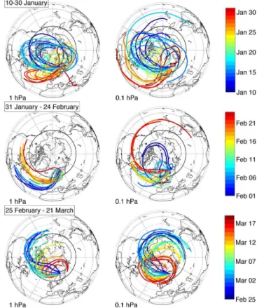
Polar projections of the 3-day backward trajectories started over Sodankyl¨a at 1 hPa (left column) and 0.1 hPa (right column) are displayed in Fig. 10. Trajectories follow-ing an oval shape within the polar region indicate the ex-istence of a regular eastward circulation (the polar vortex). Trajectories originating in low latitudes show low latitude air being transported towards Sodankyl¨a indicating that the po-lar vortex has either been shifted away from northern Europe or broken down.
The plots pinpoint the circulation changes described above. In mid January at both altitudes the air reaching Sodankyl¨a is following a regular circulation (polar vortex) which is disrupted by the SSW in the end of January. The dis-ruption of the circulation is associated with advection of
hu-Fig. 10.3-day LAGRANTO backward trajectories started over So-dankyl¨a at 0.1 hPa (right) and 1 hPa (left). Starting dates are divided according to the three periods defined in Sect. 5.2. Top: time of the SSW (10–30 January), middle: time of enhanced meridional mix-ing (31 January–24 February), bottom: time of the USLM vortex (25 February–21 March). The colors of the trajectories indicate the starting date, blue being the earliest, red the latest. The black circle marks 60◦N.
mid air from the subtropics to Sodankyl¨a. The reason for the increase in lower mesospheric water vapor occurring earlier in zonal mean than over Sodankyl¨a is that before the SSW the polar vortex with its dry mesospheric air was shifted towards Europe. Between the SSW and late February the circulation is still disturbed with trajectories originating at mid-latitudes following no distinct circulation pattern. This indicates large scale mixing of polar and mid-latitudinal air. In the period from early to mid-March a regular circulation has reestab-lished (USLM vortex).
Fig. 11.Latitude-altitude cross section of 20-day backward TEM Trajectories started on 15 January, 30 January, 19 February and 10 March for the altitudes 3, 1, 0.3 , 0.1 and 0.03 hPa and the latitude 67◦N. The end point of the backward trajectories is marked with a star.
the circulation changes. Now the meridional transport of mesospheric air is less pronounced while at the same time the air masses reaching the polar stratopause region have their 20-day back origin at the subtropical stratopause. This effect is associated with the strong stratospheric downwelling and simultaneous mesospheric upwelling in the polar region dur-ing the SSW. The short term water vapor increase at 0.03 and 0.1 hPa (Fig. 7), coinciding with the time of the maximum warming in the stratosphere on 30 January, is correlated with the mesospheric upwelling (Fig. 11b). Thus this water vapor increase is due to humid air transported upward from below. By 19 February (panel c) the pre-warming circulation has started to reestablish above 0.01 hPa with air masses being transported from higher altitudes at mid-latitudes. At the lower levels the TEM trajectories indicate no transport to-wards Arctic regions. This is in contrast to the Lagrangian trajectories in Fig. 10 which have their 3-day back origin in mid-latitudes throughout February. This apparent contra-diction is attributed to the presence of a planetary wave. Indications for such a wave can be seen in the Aura/MLS
Fig. 12. H2O measured by MIAWARA-C (colors, red relatively
higher values, blue relatively lower values) and WACCM-TEM backward trajectories started every 7th day at 3, 1, 0.5, 0.3, 0.1, 0.05 hPa (black lines). The trajectories are only shown when the air mass sampled is in the polar region (north of 60◦N). The vertical lines indicate the following dates (from the left): 24 January (wind reversal mesosphere), 30 January (maximum temperature at 60◦N and 10 hPa), 24 February (end of the time of enhanced meridional mixing) and 21 March (equinox).
daily mesospheric maps (not shown). Horizontal trajectories follow the wave but there will be no net meridional trans-port (and therefore no TEM) unless the conditions for non-interaction are violated. In mid-March the USLM vortex has returned and a circulation similar to before the SSW, only weaker, is present.
A qualitative comparison between the downward advec-tion as observed in MIAWARA-C’s water vapor and the ver-tical coordinate of the 67◦N TEM trajectories in the time they stay in the polar region is given in Fig. 12. The up-welling seen in the WACCM output before 30 January at altitudes above 0.1 hPa is in qualitative agreement with the increase in MIAWARA-C’s water vapor at the same time and altitude. The polar descent at altitudes above 0.1 hPa throughout February observed by MIAWARA-C is con-firmed by the vertical motion seen from the TEM trajectories. There are two complementary explanations for the delayed water vapor decrease at 0.3 hPa: (1) the polar descent at this altitude is slow throughout February, evident from the TEM trajectories, (2) above 0.3 hPa water vapor is uniformly dis-tributed after the humidification, evident from the water va-por distribution. Therefore at 0.3 hPa the slow polar descent cannot be seen in H2O VMR before the beginning of March
02 03 0.06 hPa
02 03
0.2 hPa
Des
cen
t
ra
te
[m
/d
]
-
4000 400 800
02 03
0.6 hPa
month of 2010 0
400 800 -400 0 400 800 1200
Descent rate [m/d]
0 400 800 1200
10 10 10-2
-1
0
P
res
su
re
[h
P
a]
MIAWARA-C Trajectories w*
Fig. 13.Descent (or during the SSW ascent) rates at 67◦N and over Sodankyl¨a determined from TEM trajectories (red),w∗(green) and MIAWARA-C water vapor measurements (blue horizontal lines in the left panel and blue dot in the right panel). Left panel: daily vertical motion at the indicated altitude levels; positive values indicate descent, negative values ascent. The vertical lines indicate the following dates (from the left): 24 January (wind reversal mesosphere), 30 January (maximum temperature at 60◦N and 10 hPa), 24 February (end of the time of enhanced meridional mixing) and 21 March (equinox). Right panel: mean value and standard deviation of daily descent rates between 5 February and 5 March. The solid part of the red and green curve indicates the altitude range covered by the 5.2 water vapor isopleth. The green asterisk, red and blue dots are the mean descent rates in that range found from TEM vertical wind and trajectories and determined from MIAWARA-C’s measurements, respectively.
7 Determination of the polar descent rate
The descent rate of air after the 2010 SSW over Sodankyl¨a and at 67◦N is determined on one hand from TEM vertical motions and on the other hand from MIAWARA-C and MLS water vapor observations.
From the water vapor observations the descent rate is found by a least squares linear fit to the 5.2 ppmv water vapor isopleth. Assuming a relative uncertainty of 10 % (1.2 %) for MIAWARA-C’s point measurements (MLS’s zonal mean) we get an uncertainty of the isopleth altitude of 2.5 km (0.2 km) . The determined descent rates and uncertainties are 350±40 m d−1for MIAWARA-C at Sodankyl¨a and 360± 5 m d−1for MLS zonal mean (valid for the interval 5 Febru-ary to 5 March 2010 and the pressure range 0.6 to 0.06 hPa). The results of the polynomial fits together with the original data are displayed in Fig. 6. The values found are an aver-age over altitude and time. Therefore the attribution of the descent rates to a certain altitude is imprecise.
The vertical motion from the TEM wind fields is given by either the vertical windw∗or the vertical displacement along the trajectories. The information content ofw∗and the along trajectory altitude change is slightly different;w∗ indicates vertical displacement at a fixed latitude while the TEM tra-jectories follow the latitude change of the bulk motion of air
masses. The vertical motion along the backward trajectories is calculated by taking the difference between the along tra-jectory altitudes on day 0 and day−3.
Assessment of errors in the atmospheric circulation of the WACCM model is subject to current research. Valida-tion of the polar descent rate with direct measurements of the atmospheric wind field is difficult as winds between 40 and 80 km are poorly observed with only ground based radars providing profiles at altitudes between approximately 60 and 100 km. In addition, wind measurements from satel-lites are possible between approximately 80 and 100 km, e.g. TIDI/TIMED, but suffer under large uncertainties of between 7 and 15 m s−1(Killeen et al., 2006). For that reason no errors are provided for the descent rates determined from WACCM data.
The descent rates from the TEM winds are displayed in Fig. 13 together with the value determined from MIAWARA-C’s measurements. The left panel shows daily values at three different altitudes (0.6, 0.2 and 0.06 hPa) within the range covered by the 5.2 ppmv water vapor iso-pleth. The mean descent rate determined from water vapor, shown as blue horizontal line, is an altitude average and therefore shown on all three pressure levels.
trajectory altitude change in red, for the time period in which the water vapor data has been considered for the linear fit (5 February to 5 March). The plot shows that the values of the two profiles are comparable. The descent rates from the TEM wind fields increase from approximately 80 m d−1 at 0.6 hPa to approximately 700 m d−1at 0.06 hPa. The linear fit to the 5.2 ppmv H2O isopleth provides a mean descent
rate for the covered altitude range which is shown as blue dot in the right panel of Fig. 13. In order to make the de-scent rates determined from the TEM wind fields comparable to those from water vapor the mean value is taken over the same altitude range. This results in 335 m d−1for the along trajectory altitude change (red dot) and in 325 m d−1forw∗
being in good agreement with the 350±40 m d−1found from MIAWARA-C’s measurements.
The lower mesospheric descent rates determined are slightly smaller than the values of 500 to 700 m d−1Lee et al.
(2011) and Salmi et al. (2011) found after the 2009 SSW. In addition, the upper stratospheric descent rates in 2010 are slightly smaller than those of Nassar et al. (2005) who deter-mined values of 150 m d−1after the 2004 SSW. The smaller descent rates after the 2010 SSW compared to the two other years could indicate that the vortex recovery was weaker af-ter the 2010 SSW than afaf-ter the 2004 and 2009 SSW’s.
8 Conclusions
This paper presents and interprets the evolution of meso-spheric water vapor during the SSW of January 2010 as ob-served by the ground based radiometer MIAWARA-C sta-tioned in the European Arctic. Lagrangian backward tra-jectory calculations show that the strong increase in meso-spheric H2O in the beginning of the SSW is associated with
meridional advection of humid air from mid-latitudes. At the time of maximum temperature in the stratosphere there is a short term water vapor increase in the upper mesosphere (0.1 and 0.03 hPa) of nearly 1 ppmv over Sodankyl¨a which is attributed to upwelling of humid air from lower altitudes. The upwelling is evident from the output of the SD-WACCM simulation and is indirectly confirmed by MIAWARA-C’s water vapor observations.
After the SSW the northern middle atmosphere was dis-turbed for approximately 3 weeks. Lagrangian backward tra-jectories started above Sodankyl¨a originated in middle lati-tudes and the MLS zonal mean distribution of water vapor indicated strong mixing. At the same time the SD-WACCM TEM trajectories showed no large scale advection of air masses from middle latitudes towards the Arctic. In March a weak vortex reestablished in the USLM region and the TEM circulation returned to a pattern similar to pre-SSW condi-tions. The rates of polar winter descent after the SSW deter-mined from water vapor measurements are 350±40 m d−1 over Sodankyl¨a (MIAWARA-C) and 360±5 m d−1in zonal mean at 67◦N (Aura/MLS). These values are consistent with
the 335 m d−1altitude change along the TEM trajectories and
the 325 m d−1residual vertical wind from SD-WACCM. This
shows that point measurements obtained from ground based microwave radiometers are well suited to detect and quantify dynamical large scale phenomena such as polar descent.
The combination of ground based and space borne mi-crowave radiometers, Lagrangian trajectories from ECMWF operational data and SD-WACCM model data gave detailed results on transport processes in the polar winter atmosphere before, during and after the SSW of January 2010. There is a good agreement between polar descent as observed in MIAWARA-C’s water vapor and the vertical component of the 67◦N TEM trajectories (shown in Fig. 12). The simi-lar mean descent rates indicate that the dynamics in the SD-WACCM model is consistent with the H2O observations.
This study shows that the main features of transport dur-ing the SSW 2010 are reflected in the water vapor measure-ments by MLS as well as by MIAWARA-C. Ground based microwave radiometers can be used to study short term dy-namical phenomena such as SSWs if their data is comple-mented with global fields from space borne instruments or models. Instrumental improvement of the ground based ra-diometers operated by the microwave group in Bern achieved in the past year has led to an increase in temporal resolution. The radiometers now deliver profiles approximately every 4 h which allows future studies of even shorter term phenomena such as atmospheric tides.
Acknowledgements. This work has been supported by the Swiss National Science Foundation grant number 200020-134684.
Participation at the Lapbiat campaign was funded through the EU Sixth Framework Program, Lapland Atmosphere-Biosphere Facil-ity (LAPBIAT2). We thank the team of the Finnish Weather Service for their hospitality and support during the campaign.
In addition we thank Dominik Scheiben for providing a MATLAB interface to LAGRANTO and Mark Whale for correcting the En-glish.
Particularly we like to thank the Bern University Research Founda-tion for funding the weather staFounda-tion of MIAWARA-C.
The National Center for Atmospheric Research is sponsored by the National Science Foundation.
Edited by: W. Ward
References
Allen, D. R., Stanford, J. L., Nakamura, N., L´opez-Valverde, M. A., L´opez-Puertas, M., Taylor, F. W., and Remedios, J. J.: Antarctic polar descent and planetary wave activity observed in ISAMS CO from April to July 1992, Geophys. Res. Lett., 27, 665–668, doi:10.1029/1999GL010888, 2000.
doi:10.1175/1520-0469(1976)033<2031:PWIHAV>2.0.CO;2, 1976.
Andrews, D. G., Holton, J. R., and Leovy, C. B.: Middle atmosphere dynamics, Academic Press, Inc., London, 1987.
Brasseur, G. P. and Solomon, S.: Aeronomy of the Middle Atmo-sphere, Springer, 3300 AA Dordrecht, Netherlands, third revised and enlarged edition, 2005.
Brewer, A. W.: Evidence for a world circulation provided by the measurements of helium and water vapour distribution in the stratosphere, Q. J. Roy. Meteorol. Soc., 75, 351–363, doi:10.1002/qj.49707532603, 1949.
Charlton, A. J. and Polvani, L. M.: A New Look at Stratospheric Sudden Warmings. Part I: Climatology and Modeling Bench-marks, J. Climate, 20, 449–469, doi:10.1175/JCLI3996.1, 2006. Coy, L., Eckermann, S., and Hoppel, K.: Planetary Wave Break-ing and Tropospheric ForcBreak-ing as Seen in the Stratospheric Sudden Warming of 2006, J. Atmos. Sci., 66, 495–507, doi:10.1175/2008JAS2784.1, 2009.
de Wachter, E., Hocke, K., Flury, T., Scheiben, D., K¨ampfer, N., Ka, S., and Oh, J. J.: Signatures of the Sudden Stratospheric Warming events of January–February 2008 in Seoul, S. Korea, Adv. Space Res., 48, 1631–1637, doi:10.1016/j.asr.2011.08.002, 2011. ECMWF: IFS documentation for cycle 36r1, http://www.ecmwf.int/
research/ifsdocs/CY36r1/index.html, 2012a.
ECMWF: Evolution – Revisions during 2010, http: //www.ecmwf.int/products/data/operational system/evolution/ evolution 2010.html, last access: 20 June 2012b.
Flury, T., Hocke, K., Haefele, A., K¨ampfer, N., and Lehmann, R.: Ozone depletion, water vapor increase, and PSC generation at midlatitudes by the 2008 major stratospheric warming, J. Geo-phys. Res., 114, D18302, doi:10.1029/2009JD011940, 2009. Forkman, P., Eriksson, P., Murtagh, D., and Espy, P.: Observing the
vertical branch of the mesospheric circulation at latitude 60◦N using ground-based measurements of CO and H2O, J. Geophys.
Res., 110, D05107, doi:10.1029/2004JD004916, 2005.
Funke, B., L´opez-Puertas, M., Bermejo-Pantale´on, D., Garc´ıa-Comas, M., Stiller, G. P., von Clarmann, T., Kiefer, M., and Linden, A.: Evidence for dynamical coupling from the lower atmosphere to the thermosphere during a ma-jor stratospheric warming, Geophys. Res. Lett., 37, L13803, doi:10.1029/2010GL043619, 2010.
Harada, Y., Goto, A., Hasegawa, H., Fujikawa, N., Naoe, H., and Hirooka, T.: A Major Stratospheric Sudden Warm-ing Event in January 2009, J. Atmos. Sci., 67, 2052–2069, doi:10.1175/2009JAS3320.1, 2010.
Killeen, T. L., Wu, Q., Solomon, S. C., Ortland, D. A., Skinner, W. R., Niciejewski, R. J., and Gell, D. A.: TIMED Doppler In-terferometer: Overview and recent results, J. Geophys. Res., 111, A10S01, doi:10.1029/2005JA011484, 2006.
Kinnison, D. E., Brasseur, G. P., Walters, S., Garcia, R. R., Marsh, D. R., Sassi, F., Harvey, V. L., Randall, C. E., Emmons, L., Lamarque, J. F., Hess, P., Orlando, J. J., Tie, X. X., Randel, W., Pan, L. L., Gettelman, A., Granier, C., Diehl, T., Niemeier, U., and Simmons, A. J.: Sensitivity of chemical tracers to meteoro-logical parameters in the MOZART-3 chemical transport model, J. Geophys. Res., 112, D20302, doi:10.1029/2006JD007879, 2007.
Lamarque, J.-F., Emmons, L. K., Hess, P. G., Kinnison, D. E., Tilmes, S., Vitt, F., Heald, C. L., Holland, E. A., Lauritzen,
P. H., Neu, J., Orlando, J. J., Rasch, P. J., and Tyndall, G. K.: CAM-chem: description and evaluation of interactive at-mospheric chemistry in the Community Earth System Model, Geosci. Model Dev., 5, 369–411, doi:10.5194/gmd-5-369-2012, 2012.
Lambert, A., Read, W. G., Livesey, N. J., Santee, M. L., Manney, G. L., Froidevaux, L., Wu, D. L., Schwartz, M. J., Pumphrey, H. C., Jimenez, C., Nedoluha, G. E., Cofield, R. E., Cuddy, D. T., Daffer, W. H., Drouin, B. J., Fuller, R. A., Jarnot, R. F., Knosp, B. W., Pickett, H. M., Perun, V. S., Snyder, W. V., Stek, P. C., Thurstans, R. P., Wagner, P. A., Waters, J. W., Jucks, K. W., Toon, G. C., Stachnik, R. A., Bernath, P. F., Boone, C. D., Walker, K. A., Urban, J., Murtagh, D., Elkins, J. W., and Atlas, E.: Vali-dation of the Aura Microwave Limb Sounder middle atmosphere water vapor and nitrous oxide measurements, J. Geophys. Res., 112, D24S36, doi:10.1029/2007JD008724, 2007.
Leblanc, T., Walsh, T. D., McDermid, I. S., Toon, G. C., Blavier, J.-F., Haines, B., Read, W. G., Herman, B., Fetzer, E., Sander, S., Pongetti, T., Whiteman, D. N., McGee, T. G., Twigg, L., Sum-nicht, G., Venable, D., Calhoun, M., Dirisu, A., Hurst, D., Jordan, A., Hall, E., Miloshevich, L., V¨omel, H., Straub, C., Kampfer, N., Nedoluha, G. E., Gomez, R. M., Holub, K., Gutman, S., Braun, J., Vanhove, T., Stiller, G., and Hauchecorne, A.: Mea-surements of Humidity in the Atmosphere and Validation Exper-iments (MOHAVE)-2009: overview of campaign operations and results, Atmos. Meas. Tech., 4, 2579–2605, doi:10.5194/amt-4-2579-2011, 2011.
Lee, J. N., Wu, D. L., Manney, G. L., Schwartz, M. J., Lambert, A., Livesey, N. J., Minschwander, K. R., Pumphrey, H. C., and Read, W. G.: Aura Microwave Limb Sounder observations of the polar middle atmosphere: Dynamics and transport of CO and H2O, J.
Geophys. Res., 116, D05110, doi:10.1029/2010JD014608, 2011. Liu, H. L. and Roble, R. G.: A study of a self-generated strato-spheric sudden warming and its mesostrato-spheric-lower thermo-spheric impacts using the coupled TIME-GCM/CCM3, J. Geo-phys. Res., 107, D23, doi:10.1029/2001JD001533, 2002. Liu, H.-L., Sassi, F., and Garcia, R. R.: Error Growth in a
Whole Atmosphere Climate Model, J. Atmos. Sci., 66, 173–186, doi:10.1175/2008JAS2825.1, 2008.
Manney, G. L., Zurek, R. W., O’Neill, A., and Swinbank, R.: On The Motion Of Air Through The Stratospheric Polar Vortex, J. Atmos. Sci., 51, 2973–2994, 1994.
Manney, G. L., Kr¨uger, K., Pawson, S., Minschwaner, K., Schwartz, M. J., Daffer, W. H., Livesey, N., Mlynczak, M. G., Rems-berg, E. E., Russell, J. M., and Waters, J. W.: The evolution of the stratopause during the 2006 major warming: Satellite data and assimilated meteorological analyses, J. Geophys. Res., 113, D11115, doi:10.1029/2007JD009097, 2008.
Manney, G. L., Harwood, R. S., MacKenzie, I. A., Minschwaner, K., Allen, D. R., Santee, M. L., Walker, K. A., Hegglin, M. I., Lambert, A., Pumphrey, H. C., Bernath, P. F., Boone, C. D., Schwartz, M. J., Livesey, N. J., Daffer, W. H., and Fuller, R. A.: Satellite observations and modeling of transport in the upper tro-posphere through the lower mesosphere during the 2006 major stratospheric sudden warming, Atmos. Chem. Phys., 9, 4775– 4795, doi:10.5194/acp-9-4775-2009, 2009a.
the Record-breaking 2009 Arctic Stratospheric Major Warming, Geophys. Res. Lett., 36, L12815, doi:10.1029/2009GL038586, 2009b.
Matsuno, T.: A Dynamical Model of the Stratospheric Sudden Warming., J. Atmos. Sci., 28, 1479–1494, doi:10.1175/1520-0469(1971)028<1479:ADMOTS>2.0.CO;2, 1971.
Monge-Sanz, B. M., Chipperfield, M. P., Simmons, A. J., and Up-pala, S. M.: Mean age of air and transport in a CTM: Comparison of different ECMWF analyses, Geophys. Res. Lett., 34, L04801, doi:10.1029/2006GL028515, 2007.
Nassar, R., Bernath, P. F., Boone, C. D., Manney, G. L., McLeod, S. D., Rinsland, C. P., Skelton, R., and Walker, K. A.: ACE-FTS measurements across the edge of the winter 2004 Arctic vortex, Geophys. Res. Lett., 32, L15S05, doi:10.1029/2005GL022671, 2005.
Nezlin, Y., Rochon, Y. J., and Polavarapu, S.: Impact of tropospheric and stratospheric data assimilation on mesospheric prediction, Tellus A, 61, 154–159, doi:10.1111/j.1600-0870.2008.00368.x, 2009.
Orsolini, Y. J., Urban, J., Murtagh, D., Lossow, S., and Limpasuvan, V.: Descent from the polar mesosphere and anomalously high stratopause observed in 8 years of water vapor and temperature satellite observations by the Odin Sub-Millimeter Radiometer, J. Geophys. Res., 115, D12305, doi:10.1029/2009JD013501, 2010. Richter, J. H., Sassi, F., and Garcia, R. R.: Toward a Phys-ically Based Gravity Wave Source Parameterization in a General Circulation Model, J. Atmos. Sci., 67, 136–156, doi:10.1175/2009JAS3112.1, 2010.
Salmi, S.-M., Verronen, P. T., Th¨olix, L., Kyr¨ol¨a, E., Backman, L., Karpechko, A. Yu., and Sepp¨al¨a, A.: Mesosphere-to-stratosphere descent of odd nitrogen in February-March 2009 after sudden stratospheric warming, Atmos. Chem. Phys., 11, 4645–4655, doi:10.5194/acp-11-4645-2011, 2011.
Seele, C. and Hartogh, P.: A case study on middle atmo-spheric water vapor transport during the February 1998 stratospheric warming, Geophys. Res. Lett., 27, 3309–3312, doi:10.1029/2000GL011616, 2000.
Siskind, D. E., Eckermann, S. D., Coy, L., McCormack, J. P., and Randall, C. E.: On recent interannual variability of the Arctic winter mesosphere: Implications for tracer descent, Geophys. Res. Lett., 34, L09806, doi:10.1029/2007GL029293, 2007. Siskind, D. E., Eckermann, S. D., McCormack, J. P., Coy,
L., Hoppel, K. W., and Baker, N. L.: Case studies of the mesospheric response to recent minor, major, and ex-tended stratospheric warmings, J. Geophys. Res., 115, D00N03, doi:10.1029/2010JD014114, 2010.
Smith, A. K. K., Garcia, R. R., Marsh, D. R. R., and Richter, J. H.: WACCM Simulations of the Mean Circulation and Trace Species Transport in the Winter Mesosphere, J. Geophys. Res., 116, D20115, doi:10.1029/2011JD016083, 2011.
SPARC: Report on the Evaluation of Chemistry-Climate Models, in: Stratospheric Processes And their Role in Climate (SPARC), Report No. 5, edited by: Eyring, V., Shepherd, T. G., and Waugh, D. W., WCRP-132, WMO/TD-No. 1526, http://www.atmosp. physics.utoronto.ca/SPARC, 2010.
Stiller, G. P., Kiefer, M., Eckert, E., von Clarmann, T., Kellmann, S., Garc´ıa-Comas, M., Funke, B., Leblanc, T., Fetzer, E., Froide-vaux, L., Gomez, M., Hall, E., Hurst, D., Jordan, A., K¨ampfer, N., Lambert, A., McDermid, I. S., McGee, T., Miloshevich, L., Nedoluha, G., Read, W., Schneider, M., Schwartz, M., Straub, C., Toon, G., Twigg, L. W., Walker, K., and Whiteman, D. N.: Vali-dation of MIPAS IMK/IAA temperature, water vapor, and ozone profiles with MOHAVE-2009 campaign measurements, Atmos. Meas. Tech., 5, 289–320, doi:10.5194/amt-5-289-2012, 2012. Straub, C., Murk, A., and K¨ampfer, N.: MIAWARA-C, a new
ground based water vapor radiometer for measurement cam-paigns, Atmos. Meas. Tech., 3, 1271–1285, doi:10.5194/amt-3-1271-2010, 2010.
Straub, C., Murk, A., K¨ampfer, N., Golchert, S. H. W., Hochschild, G., Hallgren, K., and Hartogh, P.: ARIS-Campaign: intercom-parison of three ground based 22 GHz radiometers for middle atmospheric water vapor at the Zugspitze in winter 2009, At-mos. Meas. Tech., 4, 1979–1994, doi:10.5194/amt-4-1979-2011, 2011.
Waters, J., Froidevaux, L., Harwood, R., Jarno, R., Pickett, H., Read, W., Siegel, P., Cofield, R., Filipiak, M., Flower, D., Holden, J., Lau, G., Livesey, N., Manney, G., Pumphrey, H., Santee, M., Wu, D., Cuddy, D., Lay, R., Loo, M., Perun, V., Schwartz, M., Stek, P., Thurstans, R., Boyles, M., Chandra, S., Chavez, M., Chen, G.-S., Chudasama, B., Dodge, R., Fuller, R., Girard, M., Jiang, J., Jiang, Y., Knosp, B., LaBelle, R., Lam, J., Lee, K., Miller, D., Oswald, J., Patel, N., Pukala, D., Quintero, O., Scaff, D., Snyder, W., Tope, M., Wagner, P., and Walch, M.: The Earth Observing System Microwave Limb Sounder (EOS MLS) on the Aura satellite, IEEE T. Geosci. Remote Sens., 44, 1075–1092, 2006.