Transport of mesospheric H<sub>2</sub>O during and after the stratospheric sudden warming of January 2010: observation and simulation

(1)

ACPD

11, 32811–32846, 2011

SSW 2010 – transport of mesospheric H₂O

C. Straub et al.

Title Page

Abstract Introduction

Conclusions References

Tables Figures

◭ ◮

Back Close

Full Screen / Esc

Printer-friendly Version

Interactive Discussion

Discussion

P

a

per

|

Dis

cussion

P

a

per

|

Discussion

P

a

per

|

Discussio

n

P

a

per

|

Atmos. Chem. Phys. Discuss., 11, 32811–32846, 2011 www.atmos-chem-phys-discuss.net/11/32811/2011/ doi:10.5194/acpd-11-32811-2011

Atmospheric Chemistry and Physics Discussions

This discussion paper is/has been under review for the journal Atmospheric Chemistry and Physics (ACP). Please refer to the corresponding final paper in ACP if available.

Transport of mesospheric H

₂

O during and

after the stratospheric sudden warming of

January 2010: observation and simulation

C. Straub1, B. Tschanz1, K. Hocke1,2, N. K ¨ampfer1,2, and A. K. Smith3

1

Institute of Applied Physics, University of Bern, Bern, Switzerland 2

Oeschger Center for Climate Change Research, University of Bern, Bern, Switzerland 3

Atmospheric Chemistry Division, National Center for Atmospheric Research, Boulder, CO, USA

Received: 20 October 2011 – Accepted: 1 December 2011 – Published: 12 December 2011

Correspondence to: C. Straub ([email protected])

(2)

ACPD

11, 32811–32846, 2011

C. Straub et al.

Title Page

Tables Figures

◭ ◮

Back Close

Full Screen / Esc

Discussion

P

a

per

|

Dis

cussion

P

a

per

|

Discussion

P

a

per

|

Discussio

n

P

a

per

|

Abstract

The transportable ground based microwave radiometer MIAWARA-C monitored the upper stratospheric and lower mesospheric (USLM) water vapor distribution over

So-dankyl ¨a, Finland (67.4◦N, 26.6◦N) from January to June 2010. At the end of January,

approximately 2 weeks after MIAWARA-C’s start of operation in Finland, a stratospheric

5

sudden warming (SSW) disturbed the circulation of the middle atmosphere. Shortly af-ter the onset of the SSW waaf-ter vapor in the USLM rapidly increased from approximately 5.5 to 7 ppmv in the end of January. Backward trajectory calculations show that this strong increase is due to the break down of the polar vortex and meridional advec-tion of subtropical air to the arctic USLM region. In addiadvec-tion, mesospheric upwelling in

10

the course of the SSW led to an increase in observed water vapor between 0.1 and 0.03 hPa.

After the SSW MIAWARA-C observed a decrease in mesospheric water vapor

vol-ume mixing ratio (VMR) due to the subsidence of H₂O poor air masses in the polar

region. Backward trajectory analysis and the zonal mean water vapor distribution from

15

the Microwave Limb Sounder on the Aura satellite (Aura/MLS) indicate the occurrence

of two regimes of circulation from 50◦_{N to the north pole: 1) regime of enhanced}

merid-ional mixing throughout February and 2) regime of an eastward circulation in the USLM region reestablished between early March and equinox. The polar descent rate

deter-mined from MIAWARA-C’s 5.2 ppmv isopleth is 350 m d−1 _{in the pressure range 0.6 to}

20

0.06 hPa between mid February and early March. For the same time interval the de-scent rate was determined using trajectories calculated from the Transformed Eulerian Mean (TEM) wind fields simulated by means of the Whole Atmosphere Community

Climate Model (WACCM). The values found using these different methods are in good

agreement.

(3)

ACPD

11, 32811–32846, 2011

C. Straub et al.

Title Page

Tables Figures

◭ ◮

Back Close

Full Screen / Esc

Discussion

P

a

per

|

Dis

cussion

P

a

per

|

Discussion

P

a

per

|

Discussio

n

P

a

per

|

1 Introduction

Water vapor enters the stratosphere from the equatorial troposphere through the trop-ical tropopause layer (TTL) from where it is transported upward into the mesosphere following the Brewer-Dobson circulation (Andrews et al., 1987). As the TTL acts as a cold trap the whole middle atmosphere is extremely dry (Brewer, 1949). The positive

5

vertical gradient throughout the stratosphere is due to the second source of H2O in the

middle atmosphere, the oxidation of methane while the negative vertical gradient in the

mesosphere is caused by photo-dissociation due to the absorption of solar Lymanα

radiation.

The chemical lifetime of water vapor is in the order of months in the lower

meso-10

sphere and in the order of weeks in the upper mesosphere (Brasseur an Salomon, 2005). This is long with respect to dynamical processes and water vapor is therefore a tracer for atmospheric transport processes. The zonal mean distribution of water vapor in December 2009 as measured by Aura/MLS is displayed in Fig. 1. As the

vertical H2O gradient is negative throughout the mesosphere, dry air from the upper

15

atmosphere can be used to investigate polar winter descent and humid air from around the stratopause for polar summer ascent. The polar winter descent induces horizontal

gradients in the H2O VMR as the mesospheric air descending within the polar region

is much dryer than the air outside of it. Due to this horizontal gradient water vapor is a valuable tracer for short term mixing in the winter hemisphere, e.g. in the course of

20

sudden stratospheric warmings. Around the stratopause H2O is not a good tracer due

to its local maximum in the upper stratosphere.

Stratospheric sudden warmings (SSW) are extreme events in the middle atmosphere

characterized by a fast and strong increase of stratospheric temperature (at least 25◦

in a week or less) and simultaneous cooling of the mesosphere. The main cause for

25

(4)

in-ACPD

11, 32811–32846, 2011

C. Straub et al.

Title Page

Tables Figures

◭ ◮

Back Close

Full Screen / Esc

Discussion

P

a

per

|

Dis

cussion

P

a

per

|

Discussion

P

a

per

|

Discussio

n

P

a

per

|

duces a poleward residual circulation, which produces adiabatic heating due to down-ward flow in the high latitude stratosphere and adiabatic cooling due to updown-ward flow in the high latitude mesosphere.

In the course of SSWs the stratospheric polar vortex is strongly distorted and

ei-ther shifted offthe pole (vortex displacement event) or even split in two pieces (vortex

5

split event), (Charlton and Polvani, 2006). There has been a strong vortex displace-ment SSW in 2006 and a strong vortex split SSW in 2009. Both events were used to thoroughly study dynamics and transport processes during SSWs.

The criterion of a major SSW (reversal of zonal mean zonal wind and temperature

gradient north of 60◦N at 10 hPa) implies the breakdown of the polar vortex. Consistent

10

with the disappearance of the vortex transport barrier strong mixing of air masses

oc-curs. Manney et al. (2008, 2009a,b) investigated transport of the trace gases CO, H2O

and N2O during the warmings in 2006 and in 2009 using satellite data from Aura/MLS,

ACE/FTS and TIMED/SABER and model outputs from SLIMCAT, GEOS5 and ECMWF. These trace gases showed values characteristic of low and mid latitudes extending to

15

polar regions and extremely weak gradients throughout the hemisphere. Approximately 3 weeks after both the 2006 and 2009 SSWs, the vortex in the upper stratosphere and lower mesosphere (USLM) reformed, reestablishing the mixing barriers and strong dia-batic descent developed, echoing the pattern of descent typically seen in fall, (see e.g., Siskind et al., 2007; Orsolini et al., 2010; Smith et al., 2011, and references therein).

20

Using observations of Aura/MLS and Empirical Orthogonal Function (EOF) analysis

Lee et al. (2011) determined a descent rate of 400–500 m d−1 in the polar USLM

re-gion after SSWs.

There have been previous studies using data of ground based microwave radiome-ters to investigate the stratospheric and mesospheric response to SSWs. Seele and

25

(5)

ACPD

11, 32811–32846, 2011

C. Straub et al.

Title Page

Tables Figures

◭ ◮

Back Close

Full Screen / Esc

Discussion

P

a

per

|

Dis

cussion

P

a

per

|

Discussion

P

a

per

|

Discussio

n

P

a

per

|

vapor. Flury et al. (2008) investigated ozone depletion and water vapor enhancement in mid latitudes during the SSW 2008 using trajectory calculations. They showed that the water vapor enhancement is associated with meridional transport while the ozone depletion is mainly due to chemistry. de Wachter et al. (2011) observed a decrease in mesospheric water vapor over Seoul, South Korea during the SSW 2008 which they

5

attributed to polar air being transported to such low latitudes when the polar vortex was shifted towards Europe in the course of the SSW. In addition there have been studies investigating the fall descent rate in the arctic/antarctic middle atmosphere

us-ing ground based data. Forkman et al. (2005) determined 60◦N fall descent rates of

up to 300 m d−1at 75 km altitude using CO and H2O measurements while Allen et al.

10

(2000) found antarctic fall descent rates of 250 m d−1 _{at 60}◦_{S and 330 m d}−1₈₀◦_{S in} the upper stratosphere using CO data. However to our knowledge there is no study investigating polar descent after a SSW using ground based data. In this paper we do not only present post SSW arctic mesospheric descent rates determined from ground based and space borne water vapor measurements and TEM trajectory calculations

15

but also investigate horizontal transport throughout the mesosphere using backward trajectory calculations at several mesospheric altitudes.

The article is organized as follows. Sections 2 and 3 present the measured and mod-eled data sets used. Section 4 introduces the trajectory computations. Section 5 gives an overview about dynamical changes during the SSW of January 2010. Section 6

20

presents the measured water vapor distribution and discusses influences of the SSW upon it.

2 Measurement data

(6)

ACPD

11, 32811–32846, 2011

C. Straub et al.

Title Page

Tables Figures

◭ ◮

Back Close

Full Screen / Esc

Discussion

P

a

per

|

Dis

cussion

P

a

per

|

Discussion

P

a

per

|

Discussio

n

P

a

per

|

2.1 Ground based microwave radiometer MIAWARA-C

The first source is measurements of the vertical distribution of H2O VMR over

So-dankyl ¨a, Finland (67.4◦N 26.6◦E) recorded by the ground based MIddle Atmospheric

WAter vapor RAdiometer MIAWARA-C belonging to the University of Bern, Switzer-land. The instrument has been operated at the Finnish Meteorological Institute

Arc-5

tic Research Center from mid January to mid June in the frame of the Lapland Atmosphere-Biosphere Facility (LAPBIAT2) campaign. MIAWARA-C has been specif-ically designed for measurement campaigns. The instrument has two main functions; it serves as a traveling standard for inter-comparison (Straub et al., 2011; Leblanc et al., 2011; Stiller et al., 2011) and it is used in measurement campaigns focusing

10

on dynamic processes. The instrument is of a compact design and has a simple set up procedure. It can be operated as a standalone instrument as it maintains its own weather station and a calibration scheme that does not rely on other instruments or the use of liquid nitrogen. Water vapor profiles are retrieved from measured spectra of the pressure broadened 22 GHz rotational emission line (see Straub et al., 2010,

15

2011, for details on MIAWARA-C). Here, data from 10 January to 31 March 2010 is considered and analyzed to yield daily estimates of water vapor profiles in an altitude range between 10 and 0.02 hPa (approximately 30 to 75 km) with a vertical resolution of approximately 12 km.

2.2 Aura/MLS

20

The second source of data is the Microwave Limb Sounder (MLS) aboard the EOS/Aura

satellite described in Waters et al. (2006). Daily zonal averages of H2O VMR and

tem-perature MLS acquired in the Northern Hemisphere over the time interval 10 January to 31 March 2010 are considered here. The highest latitude accessible to the satellite

is 82.5◦N. MLS yields water vapor as one of its version 2.2 level 2 data products

cover-25

(7)

ACPD

11, 32811–32846, 2011

C. Straub et al.

Title Page

Tables Figures

◭ ◮

Back Close

Full Screen / Esc

Discussion

P

a

per

|

Dis

cussion

P

a

per

|

Discussion

P

a

per

|

Discussio

n

P

a

per

|

(67.4◦_{N) Aura passes at approximately 03:00 and 12:30 LT. For this analysis zonal}

mean water vapor at 67◦N is used in order to complement MIAWARA-C’s point

mea-surements with zonal mean profiles.

3 Model data 3.1 ECMWF

5

Meteorological operational reanalysis data (geopotential height, horizontal and verti-cal wind) from the European Center of Medium-range Weather Forecast (ECMWF) (Monge-Sanz et al., 2007) is used for the description of the 2010 SSW in Fig. 3 and for the Lagrangian trajectory calculations. This data set has 91 vertical levels with 9 mesospheric levels (above 1 hPa) and the upper limit at 0.01 hPa. The grid

spac-10

ing is 1.125◦ in latitude and 4.5◦ in longitude. For dynamical variables, the upper

stratosphere is constrained by space-borne radiometers. However, there is no real ob-servational constraint in the mesosphere, so that the ECMWF reanalysis data relies instead on the model and forcing from the better-analyzed areas below. In addition the mesospheric levels are relatively close to the model top. However, the model still

main-15

tains a relatively good representation of gravity wave drag processes and it produces a Brewer-Dobson circulation (A. Geer, private communication).

3.2 WACCM

This study presents results from the NCAR Whole Atmosphere Community Climate Model with Specified Dynamics (SD-WACCM). WACCM uses a free-running

dynam-20

ical core that is adopted from the NCAR Community Atmosphere Model (CAM) and a chemistry module that is an extension of version 3 of the Model of OZone And

Re-lated Tracers (MOZART3), (e.g., Kinnison et al., 2007). In a recent validation effort,

(8)

chemistry-ACPD

11, 32811–32846, 2011

C. Straub et al.

Title Page

Tables Figures

◭ ◮

Back Close

Full Screen / Esc

Discussion

P

a

per

|

Dis

cussion

P

a

per

|

Discussion

P

a

per

|

Discussio

n

P

a

per

|

climate models (SPARC, 2010). For the specified dynamics (SD) runs described in Lamarque et al. (2011), wind and temperature fields are nudged, at each model time step, using the Goddard Earth Observing System 5 (GEOS-5) analysis. The use of the specified dynamics option of WACCM facilitates the comparisons with observations of trace chemical species.

5

The gravity wave parametrization in WACCM (Richter et al., 2010) determines the mean flow forcing from a discrete spectrum of gravity waves that are forced interac-tively in the troposphere by topography, convection (mostly in low latitudes), and frontal

dynamics (middle and high latitudes). The parametrization also gives a coefficient for

vertical eddy diffusion that affects heat and the mixing ratios of trace species.

10

In the current study, SD-WACCM is nudged with 1 % of the GEOS-5 meteorologi-cal fields (e.g., temperature, zonal and meridional winds, and surface pressure) every 30 min. The nudging is applied below 50 km and tapers to zero between 50 and 60 km. The GEOS-5 analysis is available with a time resolution of 6 h and are interpolated to the 30-min nudging intervals. Latitude and longitude resolution for these WACCM runs

15

is 1.9×2.5◦and there are 88 pressure levels from the surface to 150 km altitude. The

nudging allows SD-WACCM to perform as a chemical transport model in the

tropo-sphere and stratotropo-sphere. The model generates mesospheric dynamical fields, in effect

performing as a free-running model above 60 km except that the forcing from below is based on observations.

20

4 Data analysis

This paper presents two different trajectory computation methods with two different

information contents: (1) Lagrangian backward trajectories started over Sodankyl ¨a giv-ing information on horizontal (zonal and meridional) and vertical origin of air parcels

sampled by MIAWARA-C and (2) zonal mean trajectories started at 67◦N following the

25

transformed Eulerian mean (TEM) circulation giving information on large scale

(9)

aver-ACPD

11, 32811–32846, 2011

C. Straub et al.

Title Page

Tables Figures

◭ ◮

Back Close

Full Screen / Esc

Discussion

P

a

per

|

Dis

cussion

P

a

per

|

Discussion

P

a

per

|

Discussio

n

P

a

per

|

aged winds and wave momentum transport.

4.1 Lagrangian backward trajectories

The Lagrangian backward trajectories are computed using the three-dimensional LA-GRangian ANalysis TOol LAGRANTO described in Wernli and Davies (1996) together with the wind fields provided by ECMWF operational data. A possible drawback for

5

mesospheric trajectories is the inaccuracy of the wind fields (especially vertical wind) increasing towards the upper edge of the ECMWF model grid at 0.01 hPa.

Daily backward trajectories are calculated for every USLM pressure level of

MIAWARA-C’s retrieval grid. As the photo-chemical lifetime of H₂O is in the order

of months in the lower mesosphere and weeks in the upper mesosphere its VMR is

as-10

sumed to be conserved along the trajectory. The trajectories give us the geographical origin of the air masses measured by MIAWARA-C.

As there is no observational information on upper stratospheric and mesospheric water vapor in the ECMWF system the water vapor values along the trajectories are determined from MLS observations. This is done in a very basic way: we search for

15

all the MLS profiles on the according day that are acquired within±1◦ in latitude and

±10◦in longitude of the air parcel’s location and take the mean value of the H2O VMR

at each MLS pressure level. The value closest to the altitude of the air parcel is the water vapor VMR used.

As the displacement of single air parcels by the mesospheric circulation is rapid this

20

study presents 3-day LAGRANTO backward trajectories.

4.2 TEM backward trajectories

The TEM circulation describes the bulk motion of large scale air masses as it closely approximates the net air parcel displacement in the latitude-pressure plane (Andrews and McIntyre, 1976). The two dimensional TEM trajectories are calculated using daily

25

(10)

ACPD

11, 32811–32846, 2011

C. Straub et al.

Title Page

Tables Figures

◭ ◮

Back Close

Full Screen / Esc

Discussion

P

a

per

|

Dis

cussion

P

a

per

|

Discussion

P

a

per

|

Discussio

n

P

a

per

|

reliable than ECMWF in the mesosphere because it has an upper limit near 150 km and includes representation of the dynamical and energetic processes that are important in the mesosphere and lowermost thermosphere. The approach used for the trajectory computations is the exact same as in Smith et al. (2011). For the presented

analy-sis the daily backward trajectories are started at 67◦N for every USLM pressure level

5

of MIAWARA-C’s retrieval grid. For the illustration of short term vertical motion 3 day backward trajectory calculation are shown and 20 day backward TEM trajectories are presented in order to illustrate the residual meridional circulation (Brewer-Dobson cir-culation).

5 The SSW 2010

10

5.1 Dynamical overview

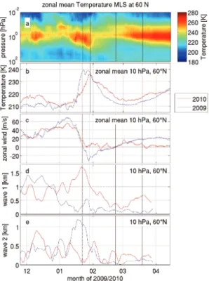
The temperature and wind evolution of the 2010 SSW was similar to the major SSW of late January 2009 described in Manney et al. (2009b). The polar stratopause dropped and broke down (nearly isothermal middle atmosphere) and then reformed at a high

altitude (∼0.03 hPa). As this effect is most pronounced at latitudes above 70◦N the

15

temperature evolution at 80◦N is displayed in the upper panel of Fig. 2. The lower

panel shows the temporal evolution of ECMWF zonal mean zonal wind at the

approx-imate latitude of the polar night jet (60◦N). In December and January the polar night

jet is visible as a westerly (eastward) circulation centered around 60◦N and 1 hPa. By

the end of January it is rapidly decelerated, the polar vortex is shifted towards Europe

20

and the zonal mean temperature at 10 hPa and 60◦N increases by approximately 25 K

with the maximum on 30 January (second vertical line in the figures). The zonal mean latitudinal temperature gradient is positive in that time. The zonal mean wind reverses

at altitudes above 10 hPa and latitudes north of 60◦N on 24 January (first vertical line

in the figures) with maximum wind speeds of 60 m s−1

at 0.3 hPa and 65◦_{N on 29}

25

(11)

ACPD

11, 32811–32846, 2011

C. Straub et al.

Title Page

Tables Figures

◭ ◮

Back Close

Full Screen / Esc

Discussion

P

a

per

|

Dis

cussion

P

a

per

|

Discussion

P

a

per

|

Discussio

n

P

a

per

|

polar vortex does not recover before the circulation reverses to summer easterlies in the end of March (Fig. 2). In the mesosphere an eastward circulation returns approxi-mately 10 days after the wind reversal and by the end of February a USLM vortex forms reestablishing a weak mixing barrier. This is similar to the evolution observed after the SSW 2009 (Manney et al., 2009b) except for the fact that in 2010 the post SSW USLM

5

vortex remained weaker than in 2009.

In order to point out similarities and differences a direct comparison between the

SSW of January 2010 (red line) and the SSW of January 2009 (blue line) is given in panels b, c, d and e of Fig. 3. As the two warmings occurred at a similar time of the year the same axis showing month of 2008/2009 or 2009/2010, respectively is used for

10

both lines. This figure is loosely based on Fig. 1 in Manney et al. (2009b) comparing the SSWs of 2006 and 2009. In January 2009 the anomalous increase in stratospheric temperature was faster and slightly stronger than in 2010. The same is true for the

deceleration of the zonal mean zonal wind at 60◦_{N and 10 hPa. In 2009 the zonal wind}

reversal was accompanied by strong geopotential height wave 2 amplification (vortex

15

split event) while geopotential height wave 1 was strong in December but weakened in the beginning of January. A few days after the maximum temperature a slight wave 1 amplification was evident. In the beginning of winter 2009/2010 geopotential height wave 1 was weaker than at the same time of the previous year but it amplified before the SSW in January at the same time as the zonal mean zonal wind decelerated. This

20

indicates that the January 2010 SSW was a vortex displacement event. The amplitude of wave 2 had a peak in mid-December when a minor SSW occurred but stayed fairly weak for the rest of the winter.

5.2 Zonal mean water vapor distribution indicating horizontal mixing and vertical motion

25

(12)

po-ACPD

11, 32811–32846, 2011

C. Straub et al.

Title Page

Tables Figures

◭ ◮

Back Close

Full Screen / Esc

Discussion

P

a

per

|

Dis

cussion

P

a

per

|

Discussion

P

a

per

|

Discussio

n

P

a

per

|

lar night jet is clearly visible in the form of a maximum in westerly wind at 60◦_{N and}

1 hPa and a strong horizontal gradient in mesospheric water vapor VMR with dry air

north of 60◦N and humid air south of it (panel a). During the SSW, on the day of the

maximum warming/cooling in the stratosphere/mesosphere the situation has reversed: now the middle atmospheric zonal wind in the arctic has changed to easterly and the

5

mesosphere (at altitudes above 0.1 hPa) is more humid north of 60◦N than south of

it (panel b). This situation is short lived and only persists for 3 days. It is linked with the strong mesospheric upwelling in the course of the SSW leading to the observed cooling above 0.1 hPa.

For approximately three weeks after the warming the mean horizontal water vapor

10

distribution in the mesosphere at latitudes between 45 and 82.5◦N is close to uniform

and the maximum in zonal mean westerly wind is situated at approximately 40◦N in

the mesosphere (panel c shows the 19 February as an example). The disappearance

of meridional H2O gradients indicates strong horizontal mixing between mid-latitudes

and the Arctic. Approximately four weeks after the SSW the horizontal H2O gradient

15

at around 60◦_{N has reappeared and the zonal mean zonal westerly wind shows a}

maximum at 55◦N and 0.1 hPa indicating that the mixing barrier has reformed (panel

d shows 10 March). However, the mid-latitude mesosphere especially at altitudes be-tween 0.1 and 0.03 hPa is now dryer than before the warming.

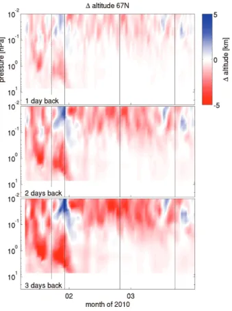
Vertical motion of air along WACCM TEM backward trajectories started at 67◦N is

20

shown in Fig. 5. The plot displays altitude changes of air against time and pressure for

different transport durations (1, 2 and 3 days). Polar mid-winter 2010 is (as expected)

mostly dominated by subsidence of air (red colors) with the exception of the time dur-ing the SSW when upwelldur-ing in the mesosphere is evident from the blue colored area between 24 January and 7 February in Fig. 5. The upwelling appears to start in the

25

(13)

ACPD

11, 32811–32846, 2011

C. Straub et al.

Title Page

Tables Figures

◭ ◮

Back Close

Full Screen / Esc

Discussion

P

a

per

|

Dis

cussion

P

a

per

|

Discussion

P

a

per

|

Discussio

n

P

a

per

|

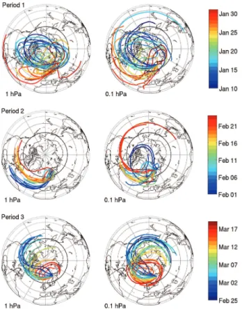
(SSW), the time between 31 January and 24 February period 2 (enhanced meridional mixing) and the time between 25 February and 21 March period 3 (USLM vortex).

6 Water vapor observations and discussion

The lower panel of Fig. 6 displays the time series of middle atmospheric water vapor over Sodankyl ¨a in winter 2010 as measured by MIAWARA-C. The upper panel shows

5

the 67◦N zonal mean water vapor obtained from MLS measurements. A direct

compar-ison between the two data sets at stratopause height (1 hPa) and three mesospheric pressure levels (0.3, 0.1 and 0.03 hPa), is given in Fig. 7. As expected the daily point measurements of MIAWARA-C show more variability than the zonal mean values of MLS. This variability is both attributed to measurement uncertainty and to small scale

10

atmospheric fluctuations (e.g. non uniform H2O distribution in combination with wind).

The distinction between the two effects is difficult and will be subject to future investi-gations.

In both time series, over Sodankyl ¨a and in zonal mean, mesospheric water vapor significantly increases by the end of January in the course of the SSW before it

de-15

creases throughout February and March. Similarities and differences in the two time

series, MIAWARA-C’s point measurements and MLS’s zonal mean, are discussed in Sects. 6.1 and 6.2.

The fact that the main features of the SSW 2010 are captured by MLS as well as MIAWARA-C shows that space borne and ground based microwave radiometers are

20

both well suited to study short term dynamical phenomena such as SSWs and at the

same time are able to monitor effects of the Brewer-Dobson circulation on middle

at-mospheric water vapor. Instrumental improvement of the ground based radiometers operated by the microwave group in Berne achieved in the past year has led to an increase in temporal resolution. The radiometers now deliver profiles approximately

25

(14)

ACPD

11, 32811–32846, 2011

C. Straub et al.

Title Page

Tables Figures

◭ ◮

Back Close

Full Screen / Esc

Discussion

P

a

per

|

Dis

cussion

P

a

per

|

Discussion

P

a

per

|

Discussio

n

P

a

per

|

In the right panel of Fig. 8 water vapor values of MIAWARA-C are compared to MLS data along the backward trajectories 1, 2 and 3 days prior to MIAWARA-C’s mea-surement. The data gaps are due to the fact that MLS provides no measurements

north of 82.5◦N. The four time series are in good agreement, especially at 0.3 and

0.1 hPa, indicating that the evolution of mesospheric water vapor can be mainly

at-5

tributed to transport processes (horizontal and vertical) and that water vapor at this altitude serves as a tracer. At the same time this good agreement provides a validation for the Lagranto/ECMWF mesospheric trajectories as the water vapor measurements are independent from the trajectory computations. At 0.03 hPa the agreement between

MIAWARA-C’s H₂O VMR and the H₂O VMR determined along the backward

trajecto-10

ries is not as good as at the lower levels. This is attributed to the fact that this pressure level is very close to the upper boundary of ECMWF at 0.01 hPa and that therefore the vertical component of the trajectories is less reliable.

6.1 Enhancement of mesospheric H2O during the SSW

6.1.1 Observation

15

At all pressure levels displayed in Fig. 7 there is an increase in humidity at the end of period 1 around the time of the SSW. This is evident over Sodankyl ¨a as well as in

the zonal mean. The effects of the 2010 SSW on mesospheric water vapor are most

pronounced at pressures between 0.3 and 0.1 hPa. Before and during the warming the humidity at 0.1 (0.3) hPa rapidly increases from approximately 5 to 7 ppmv (5.5 to

20

7 ppmv) over Sodankyl ¨a and from approximately 5 to 6 (6 to 6.5 ppmv) in zonal mean. Whereas over Sodankyl ¨a the time of the increase coincides well with the time of the zonal wind reversal (first vertical line) the increase in zonal mean occurs a few days earlier. In addition, it is noteworthy that at the time of the maximum warming in the stratosphere (second vertical line) there is a rapid increase of nearly 1 ppmv in both

25

(15)

ACPD

11, 32811–32846, 2011

C. Straub et al.

Title Page

Tables Figures

◭ ◮

Back Close

Full Screen / Esc

Discussion

P

a

per

|

Dis

cussion

P

a

per

|

Discussion

P

a

per

|

Discussio

n

P

a

per

|

6.1.2 Discussion

The meridional origin (1, 2 and 3 days back) of air masses sampled over Sodankyl ¨a against time and pressure is displayed in Fig. 8. Yellow and white colors indicate

air transported from latitudes north of 67◦_{N and orange and red colors south of it.}

Figure 8 shows that before the SSW stratospheric and lower mesospheric air over

5

Sodankyl ¨a was already in the Arctic region 3 days prior to the measurement while the origin of upper mesospheric air parcels is mostly in mid-latitudes. This is consistent with the winter mean circulation transporting upper mesospheric air from low towards high latitudes where it descends into the polar vortex (compare e.g., Smith et al., 2011). During the SSW the origin of middle atmospheric air over Sodankyl ¨a changes to

sub-10

tropical regions which is a sign of strong meridional advection towards the Arctic. The change of origin starts in the mesosphere and propagates down into the stratosphere. The first strong increase in lower mesospheric water vapor over Sodankyl ¨a coincides with the time of the mesospheric disturbance, indicating meridional advection of air from mid-latitudes. Polar projections of the 3-day backward trajectories started over

15

Sodankyl ¨a at 0.1 (left column) and 1 hPa (right column) displayed in Fig. 9 pinpoint this interpretation. Trajectories following an oval shape within the polar region indi-cate the existence of a regular eastward circulation (e.g. the polar vortex). Trajectories originating in low latitudes show low latitude air being transported towards Sodankyl ¨a indicating that the polar vortex has either been shifted away from Northern Europe or

20

broken down.

The plots show that early in period 1 at both altitudes the air reaching Sodankyl ¨a was following a regular circulation (polar vortex) which was disrupted by the SSW in the end of January. This led to advection of air from the subtropics to Sodankyl ¨a. The reason for the increase in lower mesospheric water vapor occuring earlier in zonal mean than over

25

(16)

ACPD

11, 32811–32846, 2011

C. Straub et al.

Title Page

Tables Figures

◭ ◮

Back Close

Full Screen / Esc

Discussion

P

a

per

|

Dis

cussion

P

a

per

|

Discussion

P

a

per

|

Discussio

n

P

a

per

|

short term water vapor increase at 0.03 and 0.1 hPa is correlated with the time of the maximum warming in the stratosphere and the upwelling in the mesosphere (compare Fig. 5). Thus the water vapor increase is due to humid air transported upward from below. Latitude-altitude cross section of TEM trajectories starting at altitudes of 3, 1,

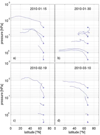
0.3, 0.1 and 0.03 hPa and latitudes of 67◦_{N are displayed in Fig. 10. Panel a indicates}

5

that before the SSW large scale air masses from high mesospheric altitudes in mid-latitude and even subtropical regions were transported into the Arctic mesosphere. The air at the stratopause and in the upper stratosphere is of polar mesospheric origin. At the time of the SSW (panel b) the circulation changes. Now the meridional transport of mesospheric air is less pronounced while at the same time the air masses reaching the

10

polar stratopause region have their 20-day back origin at the subtropical stratopause.

This effect is associated with the strong stratospheric downwelling and simultaneous

mesospheric upwelling in the polar region during the SSW.

6.2 Polar descent of H2O after the SSW

6.2.1 Observations

15

The water vapor evolution displayed in Figs. 6 and 7 indicate that after the SSW wa-ter vapor gradually decreases at mesospheric altitudes while it stays approximately constant at stratopause level.

At the highest level (0.03 hPa) the decrease from approximately 4 ppmv at the time of the maximum warming to less than 2 ppmv in mid February is very rapid both over

20

Sodankyl ¨a and in zonal mean. From the beginning of March the humidity starts to increase again.

At 0.1 hPa the H₂O VMR decreases from more than 6 to less than 4 ppmv during

February. In early March MIAWARA-C still observes a slight decrease over Sodankyl ¨a

before H2O starts to increase in mid March while in zonal average the increase already

25

(17)

ACPD

11, 32811–32846, 2011

C. Straub et al.

Title Page

Tables Figures

◭ ◮

Back Close

Full Screen / Esc

Discussion

P

a

per

|

Dis

cussion

P

a

per

|

Discussion

P

a

per

|

Discussio

n

P

a

per

|

At the lowest of the mesospheric levels (0.3 hPa) the H₂O VMR only decreases

slightly throughout February. Here the dehydration starts in early March when humidity decreases from more than 6 to less than 5 ppmv.

At stratopause level (1 hPa) water vapor stays more or less constant after the SSW with a slight decrease starting by mid March. This is in agreement with the fact that at

5

stratopause level H2O is not well suited as a tracer for horizontal or vertical advection due to the maximum in VMR at these altitudes.

6.2.2 Discussion

The meridional origin of the air masses displayed in the left panel of Fig. 8 and the polar projections in Fig. 9 indicate that between the SSW and late February (third vertical line:

10

24 February), during the time of enhanced meridional mixing (period 2), the circulation was still disturbed with mid-latitudinal air being transported to Sodankyl ¨a. However during this time the water vapor at the highest altitudes (0.1 and 0.03 hPa in Fig. 7) has already started to decrease indicating polar descent. A qualitative comparison between the downward advection as observed in MIAWARA-C’s water vapor and the

15

vertical component of the 67◦N TEM trajectories in the time they stay in the polar region is given in Fig. 11. The polar descent in period 2 at altitudes above 0.1 hPa observed by MIAWARA-C is confirmed by the vertical motion seen from the TEM trajectories.

One reason for the delayed water vapor decrease at 0.3 hPa is that polar descent at this altitude is slow throughout February, as is evident from the TEM trajectories in

20

Fig. 11. Another reason is the fact that in the altitude range above 0.3 hPa water vapor is uniformly distributed after the humidification (evident from the water vapor distribution

in Fig. 11). Therefore at 0.3 hPa the slow polar descent cannot be seen in H2O VMR

before the beginning of March due to a lack of a vertical gradient. From early to mid March Figs. 8 and 9 indicate that the air over Sodankyl ¨a is mostly of polar origin and

25

(18)

ACPD

11, 32811–32846, 2011

C. Straub et al.

Title Page

Tables Figures

◭ ◮

Back Close

Full Screen / Esc

Discussion

P

a

per

|

Dis

cussion

P

a

per

|

Discussion

P

a

per

|

Discussio

n

P

a

per

|

The TEM trajectories displayed in Fig. 10 indicate that by the end of the period of enhanced meridional mixing (panel c) the pre-warming circulation has started to reestablish at the highest level displayed with air masses coming from higher altitudes at mid-latitudes. At the lower levels the TEM trajectories indicate no transport towards Arctic regions. This is in contrast to the Lagrangian trajectories of period 2 in Fig. 9

5

which have their 3-day back origin in mid-latitudes. This apparent contradiction is at-tributed to the fact that horizontal mixing is smoothed out in the large scale advection of air masses. In mid March the USLM vortex has returned and a circulation similar to before the SSW, only weaker, is present.

6.2.3 Determination of descent rate

10

The descent rate of air after the 2010 SSW over Sodankyl ¨a and at 67◦N is determined

on one hand from the TEM trajectories and on the other hand from MIAWARA-C and MLS water vapor observations.

From the water vapor observations the downward advection is found by a linear fit to the 5.2 ppmv water vapor isopleth calculated using the contouring algorithm of

15

MATLAB. Data between 5 February and 5 March are considered for the fitting. During this time the 5.2 ppmv isopleth descents from 0.06 to 0.6 hPa. The determined descent

rates are: 350 m d−1 _{for Sodankyl ¨a and 360 m d}−1 _{in zonal mean. The result of the}

polynomial fits together with the original data are displayed in Fig. 6. These values are in good agreement with descent rates found in previous studies. They are slightly lower

20

than the descent rates of 400 to 500 m d−1 _{Lee et al. (2011) determined for the time}

after the January 2009 major SSW and slightly higher than velocities of 300 and 250–

330 m d−1 Forkman et al. (2005) and Allen et al. (2000) found for Arctic and Antarctic

fall descent, respectively.

In order to determine the vertical motion from the TEM trajectories the difference

25

between the along trajectory altitudes on consecutive days is taken. The altitude diff er-ences together with the descent rates determined from the water vapor measurements

(19)

ACPD

11, 32811–32846, 2011

C. Straub et al.

Title Page

Tables Figures

◭ ◮

Back Close

Full Screen / Esc

Discussion

P

a

per

|

Dis

cussion

P

a

per

|

Discussion

P

a

per

|

Discussio

n

P

a

per

|

good agreement. At 0.3 hPa the descent rate is slightly increasing throughout period 2 when the USLM vortex starts to reform. After the circulation has reestablished the descent rate stays constant until it starts to decrease in mid March. This is consistent with the evolution of zonal winds shown in Fig. 2.

7 Conclusions

5

This paper presents and interprets the evolution of mesospheric water vapor during the SSW 2010 as observed by the ground based radiometer MIAWARA-C stationed in the European Arctic. Lagrangian backward trajectory calculations show that the strong

increase in mesospheric H2O in the beginning of the SSW is associated with meridional

advection of humid air from mid-latitudes. At the time of maximum temperature in the

10

stratosphere there is a short term water vapor increase in the upper mesosphere of approximately 1 ppmv which is attributed to upwelling of humid air from lower altitudes. The upwelling is evident from the output of the SD-WACCM simulation and is indirectly confirmed by MIAWARA-C’s water vapor observations.

After the SSW the northern middle atmosphere was disturbed for approximately 3

15

weeks. Lagrangian backward trajectories started above Sodankyl ¨a originated in mid-dle latitudes and the MLS zonal mean distribution of water vapor indicated strong mixing. At the same time the WACCM-SD TEM trajectories showed no large scale advection of air masses from middle latitudes towards the Arctic. In March a weak vortex reestablished in the USLM region and the TEM circulation returned to a pattern

20

similar to pre-SSW conditions. The rates of polar winter descent after the SSW

deter-mined from water vapor measurements are 350 m d−1over Sodankyl ¨a (MIAWARA-C)

and 360 m d−1in zonal mean at 67◦N (Aura/MLS) and are consistent with those found

from the TEM (WACCM-SD) trajectories and by previous studies. This shows that point measurements obtained from ground based microwave radiometers are well suited to

25

(20)

ACPD

11, 32811–32846, 2011

C. Straub et al.

Title Page

Tables Figures

◭ ◮

Back Close

Full Screen / Esc

Discussion

P

a

per

|

Dis

cussion

P

a

per

|

Discussion

P

a

per

|

Discussio

n

P

a

per

|

The combination of ground based and space borne microwave radiometers, La-grangian trajectories computed from ECMWF operational data and SD-WACCM out-put gave detailed results on transport processes in the polar winter atmosphere be-fore, during and after the SSW of January 2010. Particularly the dynamics in the

SD-WACCM model is consistent with the H₂O observations and elucidates exchange

5

processes.

Acknowledgements. This work has been supported by the Swiss National Science Foundation grant number 200020-134684.

Participation at the Lapbiat campaign was funded through the EU Sixth Framework Programme, Lapland Atmosphere-Biosphere Facility (LAPBIAT2). We thank the team of the Finnish Weather 10

Service for their hospitality and support during the campaign.

In addition we thank Dominik Scheiben for providing a MATLAB interface to LAGRANTO.

Particularly we like to thank the Bern University Research Foundation for funding the weather station of MIAWARA-C.

The National Center for Atmospheric Research is sponsored by the National Science Founda-15

tion.

References

Allen, D. R., Stanford, J. L., Nakamura, N., L ´opez-Valverde, M. A., L ´opez-Puertas, M., Taylor, F. W., and Remedios, J. J.: Antarctic polar descent and planetary wave activ-ity observed in ISAMS CO from April to July 1992, Geophys. Res. Lett., 27, 665–668, 20

doi:10.1029/1999GL010888, 2000. 32815, 32828

Andrews, D. G. and McIntyre, M. E.: Planetary waves in horizontal and vertical shear: the gen-eralized eliassen-palm relation and the mean zonal acceleration, J. Atmos. Sci., 33, 2031– 2048, doi:10.1175/1520-0469(1976)033<_2031:PWIHAV>_{2.0.CO;2, 1976. 32819}

Andrews, D. G., Holton, J. R., and Leovy, C. B.: Middle Atmosphere Dynamics, Academic 25

Press, Inc., London, UK, 1987. 32813

(21)

ACPD

11, 32811–32846, 2011

C. Straub et al.

Title Page

Tables Figures

◭ ◮

Back Close

Full Screen / Esc

Discussion

P

a

per

|

Dis

cussion

P

a

per

|

Discussion

P

a

per

|

Discussio

n

P

a

per

|

Brewer, A. W.: Evidence for a world circulation provided by the measurements of helium and water vapour distribution in the stratosphere, Q. J. Roy. Meteor. Soc., 75, 351–363, doi:10.1002/qj.49707532603, 1949. 32813

Charlton, A. J. and Polvani, L. M.: A new look at stratospheric sudden warmings. Part I: Clima-tology and modeling benchmarks, J. Climate, 20, 449–469, doi:10.1175/JCLI3996.1, 2006. 5

32814

Flury, T., Hocke, K., Haefele, A., K ¨ampfer, N., and Lehmann, R.: Ozone depletion, water vapor increase, and PSC generation at midlatitudes by the 2008 major stratospheric warming, J. Geophys. Res., 114, D18302, doi:10.1029/2009JD011940, 2008. 32815

Forkman, P., Eriksson, P., Murtagh, D., and Espy, P.: Observing the vertical branch of the 10

mesospheric circulation at latitude 60◦_{N using ground-based measurements of CO and H} 2O, J. Geophys. Res., 110, D05107, doi:10.1029/2004JD004916, 2005. 32815, 32828

Kinnison, D. E., Brasseur, G. P., Walters, S., Garcia, R. R., Marsh, D. R., Sassi, F., Harvey, V. L., Randall, C. E., Emmons, L., Lamarque, J. F., Hess, P., Orlando, J. J., Tie, X. X., Randel, W., Pan, L. L., Gettelman, A., Granier, C., Diehl, T., Niemeier, U., and Simmons, A. J.: Sensi-15

tivity of chemical tracers to meteorological parameters in the MOZART-3 chemical transport model, J. Geophys. Res., 112, D20302, doi:10.1029/2006JD007879, 2007. 32817

Lamarque, J.-F., Emmons, L. K., Hess, P. G., Kinnison, D. E., Tilmes, S., Vitt, F., Heald, C. L., Holland, E. A., Lauritzen, P. H., Neu, J., Orlando, J. J., Rasch, P., and Tyndall, G.: CAM-chem: description and evaluation of interactive atmospheric chemistry in CESM, Geosci. 20

Model Dev. Discuss., 4, 2199–2278, doi:10.5194/gmdd-4-2199-2011, 2011. 32818

Leblanc, T., Walsh, T. D., McDermid, I. S., Toon, G. C., Blavier, J.-F., Haines, B., Read, W. G., Herman, B., Fetzer, E., Sander, S., Pongetti, T., Whiteman, D. N., McGee, T. G., Twigg, L., Sumnicht, G., Venable, D., Calhoun, M., Dirisu, A., Hurst, D., Jordan, A., Hall, E., Miloshe-vich, L., V ¨omel, H., Straub, C., Kampfer, N., Nedoluha, G. E., Gomez, R. M., Holub, K., Gut-25

man, S., Braun, J., Vanhove, T., Stiller, G., and Hauchecorne, A.: Measurements of Humidity in the Atmosphere and Validation Experiments (MOHAVE)-2009: overview of campaign op-erations and results, Atmos. Meas. Tech. Discuss., 4, 3277–3336, doi:10.5194/amtd-4-3277-2011, 2011. 32816

Lee, J. N., Wu, D. L., Manney, G. L., Schwartz, M. J., Lambert, A., Livesey, N. J., Minschwan-30

(22)

ACPD

11, 32811–32846, 2011

C. Straub et al.

Title Page

Tables Figures

◭ ◮

Back Close

Full Screen / Esc

Discussion

P

a

per

|

Dis

cussion

P

a

per

|

Discussion

P

a

per

|

Discussio

n

P

a

per

|

Liu, H. L. and Roble, R. G.: A study of a self-generated stratospheric sudden warming and its mesospheric-lower thermospheric impacts using the coupled TIME-GCM/CCM3, J. Geo-phys. Res., 107, 4695, doi:10.1029/2001JD001533, 2002. 32813

Manney, G. L., Kr ¨uger, K., Pawson, S., Minschwaner, K., Schwartz, M. J., Daffer, W. H., Livesey, N., Mlynczak, M. G., Remsberg, E. E., Russell, J. M., and Waters, J. W.: The evo-5

lution of the stratopause during the 2006 major warming: satellite data and assimilated me-teorological analyses, J. Geophys. Res., 113, D11115, doi:10.1029/2007JD009097, 2008. 32814

Manney, G. L., Harwood, R. S., MacKenzie, I. A., Minschwaner, K., Allen, D. R., Santee, M. L., Walker, K. A., Hegglin, M. I., Lambert, A., Pumphrey, H. C., Bernath, P. F., Boone, 10

C. D., Schwartz, M. J., Livesey, N. J., Daffer, W. H., and Fuller, R. A.: Satellite observa-tions and modeling of transport in the upper troposphere through the lower mesosphere during the 2006 major stratospheric sudden warming, Atmos. Chem. Phys., 9, 4775–4795, doi:10.5194/acp-9-4775-2009, 2009a. 32814

Manney, G. L., Schwartz, M., Krueger, K., Santee, M., Pawson, S., Lee, J., Daffer, W., Fuller, R., 15

and Livesey, N.: Aura microwave limb sounder observations of dynamics and transport dur-ing the record-breakdur-ing 2009 Arctic stratospheric major warmdur-ing, Geophys. Res. Lett., 36, L12815, doi:10.1029/2009GL038586, 2009b. 32814, 32820, 32821

Matsuno, T.: A dynamical model of the stratospheric sudden warming, J. Atmos. Sci., 28, 1479–1494, doi:10.1175/1520-0469(1971)028<1479:ADMOTS>2.0.CO;2, 1971. 32813

20

Monge-Sanz, B. M., Chipperfield, M. P., Simmons, A. J., and Uppala, S. M.: Mean age of air and transport in a CTM: comparison of different ECMWF analyses, Geophys. Res. Lett., 34, L04801, doi:10.1029/2006GL028515, 2007. 32817

Orsolini, Y. J., Urban, J., Murtagh, D., Lossow, S., and Limpasuvan, V.: Descent from the polar mesosphere and anomalously high stratopause observed in 8 years of water vapor 25

and temperature satellite observations by the Odin Sub-Millimeter Radiometer, J. Geophys. Res., 115, D12305, doi:10.1029/2009JD013501, 2010. 32814

Richter, J. H., Sassi, F., and Garcia, R. R.: Toward a physically based gravity wave source parameterization in a general circulation model, J. Atmos. Sci., 67, 136–156, doi:10.1175/2009JAS3112.1, 2010. 32818

30

(23)

ACPD

11, 32811–32846, 2011

C. Straub et al.

Title Page

Tables Figures

◭ ◮

Back Close

Full Screen / Esc

Discussion

P

a

per

|

Dis

cussion

P

a

per

|

Discussion

P

a

per

|

Discussio

n

P

a

per

|

Siskind, D. E., Eckermann, S. D., Coy, L., McCormack, J. P., and Randall, C. E.: On recent inter-annual variability of the Arctic winter mesosphere: implications for tracer descent, Geophys. Res. Lett., 34, L09806, doi:10.1029/2007GL029293, 2007. 32814

Smith, A. K. K., Garcia, R. R., Marsh, D. R. R., and Richter, J. H.: WACCM simulations of the mean circulation and trace species transport in the winter mesosphere, J. Geophys. Res., 5

116, D20115, doi:10.1029/2011JD016083, 2011. 32814, 32820, 32825

SPARC: Report on the evaluation of chemistry-climate models, in: Stratospheric Processes And their Role in Climate (SPARC), Report No. 5, edited by: Eyring, V., Shepherd, T. G., and Waugh, D. W., WCRP-132, WMO/TD-No. 1526, available at: http://www.sparc-climate.org/, 9 December 2011, 2010. 32818

10

Stiller, G. P., Kiefer, M., Eckert, E., von Clarmann, T., Kellmann, S., Garc´ıa-Comas, M., Funke, B., Leblanc, T., Fetzer, E., Froidevaux, L., Gomez, M., Hall, E., Hurst, D., Jor-dan, A., K ¨ampfer, N., Lambert, A., McDermid, I. S., McGee, T., Miloshevich, L., Nedoluha, G., Read, W., Schneider, M., Schwartz, M., Straub, C., Toon, G., Twigg, L. W., Walker, K., and Whiteman, D. N.: Validation of MIPAS IMK/IAA temperature, water vapor, and ozone profiles 15

with MOHAVE-2009 campaign measurements, Atmos. Meas. Tech. Discuss., 4, 4403–4472, doi:10.5194/amtd-4-4403-2011, 2011. 32816

Straub, C., Murk, A., and K ¨ampfer, N.: MIAWARA-C, a new ground based water vapor ra-diometer for measurement campaigns, Atmos. Meas. Tech., 3, 1271–1285, doi:10.5194/amt-3-1271-2010, 2010. 32816

20

Straub, C., Murk, A., K ¨ampfer, N., Golchert, S. H. W., Hochschild, G., Hallgren, K., and Har-togh, P.: ARIS-Campaign: intercomparison of three ground based 22 GHz radiometers for middle atmospheric water vapor at the Zugspitze in winter 2009, Atmos. Meas. Tech., 4, 1979–1994, doi:10.5194/amt-4-1979-2011, 2011. 32816

de Wachter, E., Hocke, K., Flury, T., Scheiben, D., K ¨ampfer, N., Ka, S., and Oh, J. J.: Signatures 25

of the sudden stratospheric warming events of January–February 2008 in Seoul, S. Korea, Adv. Spache Res., 48, 1631–1637, doi:10.1016/j.asr.2011.08.002, 2011. 32815

Waters, J., Froidevaux, L., Harwood, R., Jarno, R., Pickett, H., Read, W., Siegel, P., Cofield, R., Filipiak, M., Flower, D., Holden, J., Lau, G., Livesey, N., Manney, G., Pumphrey, H., San-tee, M., Wu, D., Cuddy, D., Lay, R., Loo, M., Perun, V., Schwartz, M., Stek, P., Thurstans, R., 30

(24)

ACPD

11, 32811–32846, 2011

C. Straub et al.

Title Page

Tables Figures

◭ ◮

Back Close

Full Screen / Esc

Discussion

P

a

per

|

Dis

cussion

P

a

per

|

Discussion

P

a

per

|

Discussio

n

P

a

per

|

The Earth Observing System Microwave Limb Sounder (EOS MLS) on the Aura satellite, IEEE T. Geosci. Remote, 44, 1075–1092, 2006. 32816

Wernli, H. and Davies, H. C.: A lagrangian-based analysis of extratropical cyclones. I: The method and some applications, Q. J. Roy. Meteor. Soc., 123, 467–489, doi:10.1002/qj.49712353811, 1996. 32819

(25)

ACPD

11, 32811–32846, 2011

C. Straub et al.

Title Page

Tables Figures

◭ ◮

Back Close

Full Screen / Esc

Discussion

P

a

per

|

Dis

cussion

P

a

per

|

Discussion

P

a

per

|

Discussio

n

P

a

per

|

(26)

ACPD

11, 32811–32846, 2011

C. Straub et al.

Title Page

Tables Figures

◭ ◮

Back Close

Full Screen / Esc

Discussion

P

a

per

|

Dis

cussion

P

a

per

|

Discussion

P

a

per

|

Discussio

n

P

a

per

|

(27)

ACPD

11, 32811–32846, 2011

C. Straub et al.

Title Page

Tables Figures

◭ ◮

Back Close

Full Screen / Esc

Discussion

P

a

per

|

Dis

cussion

P

a

per

|

Discussion

P

a

per

|

Discussio

n

P

a

per

|

Fig. 3. (a)MLS zonal mean temperature as function of time and pressure at 60◦_N,_(b) _MLS temperature,(c)ECMWF zonal wind,(d)altitude wave 1 from ECMWF and(e)altitude wave 2 from ECMWF. The red curves indicate temperature, zonal mean zonal wind, wave 1 and wave 2 for 2010 while the blue curve indicates corresponding values for the 2009 SSW which occurred at the almost same time of the year. For details see text.

(28)

ACPD

11, 32811–32846, 2011

C. Straub et al.

Title Page

Tables Figures

◭ ◮

Back Close

Full Screen / Esc

Discussion

P

a

per

|

Dis

cussion

P

a

per

|

Discussion

P

a

per

|

Discussio

n

P

a

per

|

(29)

ACPD

11, 32811–32846, 2011

C. Straub et al.

Title Page

Tables Figures

◭ ◮

Back Close

Full Screen / Esc

Discussion

P

a

per

|

Dis

cussion

P

a

per

|

Discussion

P

a

per

|

Discussio

n

P

a

per

|

Fig. 5. Vertical motion along WACCM TEM backward trajectories started at 67◦_{N. Altitude} changes against time and pressure 1 (top), 2 (middle), and 3 (bottom) days back compared to the starting point of the trajectory, red indicates descent and blue ascent.

(30)

ACPD

11, 32811–32846, 2011

C. Straub et al.

Title Page

Tables Figures

◭ ◮

Back Close

Full Screen / Esc

Discussion

P

a

per

|

Dis

cussion

P

a

per

|

Discussion

P

a

per

|

Discussio

n

P

a

per

|

Fig. 6. Water vapor distribution over Sodankyl ¨a as measured by MIAWARA-C (bottom) and in zonal mean at 67◦_{N as measured by MLS (top). The black line marks the polar descent of} dry mesospheric air. The descent rate is estimated as described in Sect. 6.2.3: linear fit to the 5.2 ppm isopleth of H₂O VMR for the time interval 5 February to 5 March. Descent rates are 350 m d−1for MIAWARA-C and 360 m d−1for MLS zonal mean.

(31)

ACPD

11, 32811–32846, 2011

C. Straub et al.

Title Page

Tables Figures

◭ ◮

Back Close

Full Screen / Esc

Discussion

P

a

per

|

Dis

cussion

P

a

per

|

Discussion

P

a

per

|

Discussio

n

P

a

per

|

Fig. 7. Water vapor evolution at stratopause altitude and 3 mesospheric pressure levels as observed by MIAWARA-C at 67.4◦_{N, 26.6}◦_{N and MLS zonal mean at 67}◦_N.

(32)

ACPD

11, 32811–32846, 2011

C. Straub et al.

Title Page

Tables Figures

◭ ◮

Back Close

Full Screen / Esc

Discussion

P

a

per

|

Dis

cussion

P

a

per

|

Discussion

P

a

per

|

Discussio

n

P

a

per

|

Fig. 8.Geographical origin (latitude) of measured air mass determined using Lagrangian trajec-tory calculations. The subplots show the latitude of the air 1, 2 and 3 days before MIAWARA-C samples it over Sodankyl ¨a. Water vapor VMR along the trajectories shown as time series at the same four pressure levels as in Fig. 7. Curves are H₂O VMR on the day of the measurement (blue) and the indicated amount of days earlier at the location of the sampled air mass found by the trajectories (red, green, magenta).

(33)

ACPD

11, 32811–32846, 2011

C. Straub et al.

Title Page

Tables Figures

◭ ◮

Back Close

Full Screen / Esc

Discussion

P

a

per

|

Dis

cussion

P

a

per

|

Discussion

P

a

per

|

Discussio

n

P

a

per

|

(34)

ACPD

11, 32811–32846, 2011

C. Straub et al.

Title Page

Tables Figures

◭ ◮

Back Close

Full Screen / Esc

Discussion

P

a

per

|

Dis

cussion

P

a

per

|

Discussion

P

a

per

|

Discussio

n

P

a

per

|

(35)

ACPD

11, 32811–32846, 2011

C. Straub et al.

Title Page

Tables Figures

◭ ◮

Back Close

Full Screen / Esc

Discussion

P

a

per

|

Dis

cussion

P

a

per

|

Discussion

P

a

per

|

Discussio

n

P

a

per

|

Fig. 11. H₂O measured by MIAWARA-C (colors) and WACCM-TEM backward trajectories started every 7th day at 3, 1, 0.5, 0.3, 0.1, 0.05 hPa (black lines). The trajectories are only shown when the air mass sampled is in the polar region (north of 60◦N).

(36)

ACPD

11, 32811–32846, 2011

C. Straub et al.

Title Page

Tables Figures

◭ ◮

Back Close

Full Screen / Esc

Discussion

P

a

per

|

Dis

cussion

P

a

per

|

Discussion

P

a

per

|

Discussio

n

P

a

per

|

Fig. 12. Descent (or during the SSW ascent) rates determined from TEM trajectories (dots) and water vapor measurements (horizontal line in the top panel).