Methane variations on orbital timescales: a transient modeling experiment

(1)

CPD

7, 47–77, 2011

Methane variations on orbital timescales:

a transient modeling experiment

T. Y. M. Konijnendijk et al.

Title Page

Abstract Introduction

Conclusions References

Tables Figures

◭ ◮

Back Close

Full Screen / Esc

Printer-friendly Version

Interactive Discussion

Discussion

P

a

per

|

Dis

cussion

P

a

per

|

Discussion

P

a

per

|

Discussio

n

P

a

per

|

Clim. Past Discuss., 7, 47–77, 2011 www.clim-past-discuss.net/7/47/2011/ doi:10.5194/cpd-7-47-2011

Climate of the Past Discussions

This discussion paper is/has been under review for the journal Climate of the Past (CP). Please refer to the corresponding final paper in CP if available.

Methane variations on orbital timescales:

a transient modeling experiment

T. Y. M. Konijnendijk1, S. L. Weber2,3, E. Tuenter1,3, and M. van Weele3

1

Department of Earth Sciences, Faculty of geosciences, Utrecht University, Budapestlaan 4, 3584 CD Utrecht, The Netherlands

2

Department of Physical Geography, Faculty of geosciences, Utrecht University, Heidelberglaan 2 3584 CS Utrecht, The Netherlands

3

KNMI – Royal Netherlands Meteorological Institute, Wilhelminalaan 10, 3732 GK De Bilt, The Netherlands

Received: 12 December 2010 – Accepted: 22 December 2010 – Published: 6 January 2011

Correspondence to: T. Y. M. Konijnendijk (konijnendijk@geo.uu.nl)

(2)

CPD

7, 47–77, 2011

Title Page

Tables Figures

◭ ◮

Back Close

Full Screen / Esc

Discussion

P

a

per

|

Dis

cussion

P

a

per

|

Discussion

P

a

per

|

Discussio

n

P

a

per

|

Abstract

Methane (CH4) variations on orbital timescales are often associated with variations

in wetland coverage, most notably in the summer monsoon areas of the Northern Hemisphere. Here we test this assumption by simulating orbitally forced variations in global wetland emissions, using a simple wetland distribution and CH4 emissions

5

model that was coupled off-line to a climate model containing atmosphere, ocean and vegetation components. The transient climate modeling simulation extends over the last 650 000 yrs and includes variations in land-ice distribution and greenhouse gases. Tropical temperature and global vegetation are found to be the dominant controls for global CH₄ emissions and thus atmospheric concentrations. The relative importance

10

of wetland coverage, vegetation coverage, and emission temperatures depends on the specific climatic zone (boreal, tropics and Indian/Asian monsoon area) and timescale (precession, obliquity and glacial-interglacial timescales).

Simulated variations in emissions agree well with those in measured concentrations, both in their time series and spectra. The simulated lags with respect to the orbital

15

forcing also show close agreement with those found in measured data, both on the precession and obliquity timescale. We only find covariance between monsoon pre-cipitation and CH4concentrations, however we find causal links between atmospheric

concentrations and tropical temperatures and global vegetation. The primary impor-tance of these two factors explains the lags found in the CH₄record from ice cores.

20

1 Introduction

As a greenhouse gas, methane (CH4) is a forcing factor for climate (Wang et al., 1996).

Vice versa, methane concentrations are also subjected to climate changes via changes in natural CH4production rate. The most important natural source of CH4is anaerobic

decomposition of organic material in wetlands (Fung et al., 1991). Global wetland

25

(3)

CPD

7, 47–77, 2011

Title Page

Tables Figures

◭ ◮

Back Close

Full Screen / Esc

Discussion

P

a

per

|

Dis

cussion

P

a

per

|

Discussion

P

a

per

|

Discussio

n

P

a

per

|

as temperature and vegetation (Gedney et al., 2004), is therefore key to understanding variations in the atmospheric CH4 concentration in the period before anthropogenic

influences.

Variations in CH₄ concentration have been substantial during the late Quaternary. Spahni et al. (2005) found an increase in the Epica Dome C (EDC) ice core record of

5

∼360 parts per billion by volume (ppbv) to ∼690 ppbv during the transition from Last Glacial Maximum (LGM; 21 000 yrs before present) to the Early Holocene. Long-term oscillations in the CH4 record have been linked to variations in insolation caused by

orbital forcing, particularly to the 23 000 yr (23-kyr) precession component (e.g. Rud-diman and Raymo, 2003). Strong 41-kyr and 100-kyr components are apparent also

10

in the record (Loulergue et al., 2008). These oscillations lag their respective forcing considerably. Ruddiman and Raymo (2003) devised an age model for the Vostok ice core by tuning the CH4 signal to low latitude mid-July insolation with no additional lag.

Their target curve, which is dominated by precession, e_ffectively lags 21 June 65◦_N

insolation by∼1.6 kyr. They also point out that the CH4signal has the same delayed

15

phase as northern ice sheets at the obliquity timescale.

The exact nature of the link between insolation and variations in past atmospheric CH4concentration is a much-debated topic (Schmidt et al., 2004). The most common

view on CH4 variations at orbital timescales is that Northern Hemisphere (NH)

ex-tratropical (boreal) emissions are mainly influenced by changes in temperature, while

20

tropical emissions are governed by changes in precipitation, i.e. monsoon intensity (Blunier et al., 1995). The land-sea temperature contrast that forces monsoon sys-tems is sensitive to changes in insolation, in particular the 23-kyr cycle which therefore greatly influences the strength of monsoon systems (Kutzbach et al., 2008).

Given that the bulk of emissions originates from the tropical zones with a modest

con-25

tribution from the extra-tropical NH, and negligible Southern Hemisphere (SH) emission (Walter et al., 2001; Prigent et al., 2007), it seems likely that changes in atmospheric CH4concentrations are primarily forced by changes in monsoon intensity (Chappellaz

(4)

CPD

7, 47–77, 2011

Title Page

Tables Figures

◭ ◮

Back Close

Full Screen / Esc

Discussion

P

a

per

|

Dis

cussion

P

a

per

|

Discussion

P

a

per

|

Discussio

n

P

a

per

|

compared just as favorably to reconstructed mid-latitude temperatures as they do to simulated Asian monsoon intensity. Therefore, changes in boreal emissions may well be the cause of the observed 23-kyr oscillation in atmospheric CH4.

Modeling studies have recently been performed to investigate global wetland area and associated CH₄ emissions during the LGM (Kaplan, 2002; Valdes et al., 2005;

5

Kaplan et al., 2006; Weber et al., 2010), thus implicitly focusing on the effects particular to a glacial termination Here we perform a 650 000 year transient modeling experiment, with the aim to examine the climatic origin of orbital cycles in atmospheric methane. Focus is on the precession and obliquity (41-kyr) cycles. Questions that we want to address are whether the observed cycles in CH4 originate in the tropics, in the boreal

10

zone and/or specifically in the Indian/Asian monsoon area; which climatic parameters play an important role in each of these regions; and how we can interpret the lags that have been found in the measured data with respect to the orbital forcing.

Wetland CH₄ emissions over the last 650 000 years are derived from a transient climate simulation with an atmosphere-vegetation-ocean model of intermediate

com-15

plexity (CLIMBER-2). The climate model output is used to force an off-line model that computes the global distributions of wetland area and CH₄emissions (TRENCH). Sec-tion 2 describes the models used. In Sect. 3 we analyze simulated emissions and examine the relative contribution to emission variations of the tropics, the boreal zone, and the Indian/Asian (I/A) monsoon area. The influence of changes in temperature,

20

(5)

CPD

7, 47–77, 2011

Title Page

Tables Figures

◭ ◮

Back Close

Full Screen / Esc

Discussion

P

a

per

|

Dis

cussion

P

a

per

|

Discussion

P

a

per

|

Discussio

n

P

a

per

|

2 Models and methods

2.1 The climate model

As a basis for simulating CH₄ emissions, the CLIMAte and BiosphERe model (CLIMBER-2; Petoukhov et al., 2000) was used. This is a coupled atmosphere-ocean-vegetation model of intermediate complexity that is suitable for long simulations due

5

to its fast turnaround time. The model consists of a statistical-dynamical atmosphere, which resolves the large-scale flow that arises due to spatial temperature gradients. It parameterizes atmospheric transports due to synoptic-scale variations in a sophis-ticated manner (Petoukhov et al., 2000), but it does not contain the weather events themselves. The other components are a 3-basin zonally averaged ocean, including

10

sea ice, and a terrestrial vegetation model VECODE (VEgetation COntinuous DEscrip-tion; Brovkin et al., 1997). The latter computes the fraction of the potential vegetation in a grid cell (i.e., grass, trees, and bare soil) as a function of the annual sum of positive day-temperatures and the annual precipitation. The atmospheric model of CLIMBER-2 has a resolution of 10◦in latitude and 51.43◦in longitude.

15

With CLIMBER-2 we performed a climate simulation for the interval 650 kyr BP to present, using orbital forcing (Laskar, 2004). Time-varying NH ice sheets and green-house gas concentrations (GHG) are prescribed. The volumes of the Laurentide and the Eurasian ice sheet were obtained from a 3-D ice sheet model coupled to a model of deep-ocean temperature (Bintanja et al., 2005). This model was forced by marine

20

benthic oxygen isotopes (Lisiecki and Raymo, 2005) and was run in an inverse mode resulting in timeseries of the Laurentide and Eurasian ice sheet volumes. These vol-umes were translated into a surface area and height based on the ICE-5G distribution for the LGM until present (Peltier, 2005), set on the spatial grid of CLIMBER-2. Sea level e_ffects due to changes in ice volume are not considered in this study. The

in-25

(6)

CPD

7, 47–77, 2011

Title Page

Tables Figures

◭ ◮

Back Close

Full Screen / Esc

Discussion

P

a

per

|

Dis

cussion

P

a

per

|

Discussion

P

a

per

|

Discussio

n

P

a

per

|

effect is difficult to simulate within the CLIMBER-2 grid and it is likely a minor factor in comparison to the main climate factors that are considered in this study.

GHG concentrations (CO2 and CH4) were derived from EPICA Dome C, with the

EDC-3 timescale (L ¨uthi et al., 2008; Loulergue et al., 2008). For the last 500 years we used values from several sources (Robertson et al., 2001). The total greenhouse gas

5

forcing is dominated by CO2. Therefore, the simulated climate is only determined by

the measured CH₄ concentration variations to a very limited extent. The CLIMBER-2 simulation is described in detail by Weber and Tuenter (2011).

For the present purpose of estimating wetland CH4emissions over orbital timescales

it is relevant to assess the model’s sensitivity to the different forcings involved. These

10

include both internal forcing mechanisms, such as ice sheets and greenhouse gases, as well as external orbital forcing. Compared to General Circulation Models (GCMs), the main drawback of CLIMBER-2 is obviously its coarse resolution and associated parameterizations of small-scale dynamical processes. CLIMBER-2 is however suc-cessful in simulating cold climates like the LGM (Ganopolski et al., 1998a), showing a

15

similar sensitivity and response pattern as comprehensive GCMs to the separate im-pacts of large continental ice sheets and reduced greenhouse gases (Schneider von Deimling et al., 2006). Also, the strength of the NH monsoon during an orbitally forced period like the mid-Holocene lies within the range simulated by GCMs (Ganopolski et al., 1998b; Braconnot et al., 2007). Leads and lags with respect to the orbital forcing

20

were also found to be similar to those found in more complex models (Tuenter et al., 2005; Kutzbach et al., 2008). CLIMBER-2 thus seems capable of adequately repre-senting climatic change in response to di_fferent forcings, albeit only at a large spatial scale.

2.2 CH₄emissions model

25

The wetland and CH4emission model TRENCH (TRansient Emissions of Natural CH4)

(7)

CPD

7, 47–77, 2011

Title Page

Tables Figures

◭ ◮

Back Close

Full Screen / Esc

Discussion

P

a

per

|

Dis

cussion

P

a

per

|

Discussion

P

a

per

|

Discussio

n

P

a

per

|

TRENCH consists of two consecutive components: a wetland extent algorithm and a CH4 emission algorithm. The wetland location algorithm follows the approach

origi-nally proposed by Kaplan (2002), and uses climate variables from CLIMBER-2 that are known to influence wetland formation. Wetland existence is determined based on soil moisture and soil temperature. Wetlands are assumed to exist only during months

5

when the soil temperature is above freezing point. When, in addition, a soil moisture threshold (5% of maximum saturation) is reached, a grid cell is assumed to support wetlands. The fraction of a grid cell covered by wetland is linearly related to the soil moisture value derived from CLIMBER-2 as follows:

Cwet = a × M × (1− I) (1)

10

Where Cwet is the fraction of wetland in a grid cell, a is a tuning factor, M is the soil

moisture, and I is the fraction of a grid cell covered with land ice. Resulting grid cell fractions are multiplied with the land surface area in a grid cell to obtain wetland area in km2. We assume that orography does not play a role at the present spatial resolution, as a grid cell always contains sufficient flat terrain to support wetlands when climatic

15

conditions allow this. The wetland algorithm was tuned to obtain a reasonable geo-graphical distribution of wetlands and a plausible value for worldwide wetland extent in km2, which is comparable to values in literature.

The CH4emission algorithm of TRENCH is based on Gedney et al. (2004), who

pro-pose a simple model for emissions dependent on wetland fraction, soil carbon content,

20

and temperature. The temperature sensitivity is expressed in the form of aQ10 factor.

In the present model we compute time-varying emissions for each grid cell as follows: E = k × Cwet × V ×Q

T/10

10 (2)

HereE is the CH₄ emission (in Tg CH₄ of a given grid cell at a certain time step and month,kis a tunable constant,Cwetis the fraction of wetland in a grid cell as calculated

25

in the wetland distribution model (Eq. 1), andV a vegetation factor. The temperature sensitivity is expressed in the form of aQ10 factor, with T the soil temperature in

(8)

CPD

7, 47–77, 2011

Title Page

Tables Figures

◭ ◮

Back Close

Full Screen / Esc

Discussion

P

a

per

|

Dis

cussion

P

a

per

|

Discussion

P

a

per

|

Discussio

n

P

a

per

|

The Q10 is a temperature-dependant variable itself, because the efficiency of CH4

production changes with temperature (Gedney et al., 2004). In literature, values for Q10 vary between 1.7–16 (e.g. Walter and Heimann, 2000). Most studies converge

at values around 2–4, but large differences remain as a result of different locations and covarying processes involved when calculating in theQ10 value (Segers, 1998).

5

Studies estimatingQ10 values often perform measurements on one or more wetland

sites. Because of the global scale of modeling and simplicity of the basic emission model in this study, a range ofQ10 values may be plausible. The base valueQ10(T0)

– the Q10 at 0◦C – was set at 2.0, at which value the distribution of CH4 emissions

over boreal wetlands (north of 30◦N) and tropical wetlands (latitudes between 30◦N

10

and 30◦_{S) agrees with previous observational and modeling studies.}

Wetland CH4 production also depends on the soil carbon content, which is

basi-cally the amount of decomposable organic material in the substrate (Christensen et al., 2003). As this is not simulated by the present version of CLIMBER-2, we used the grass and trees vegetation cover fractionsFgrass andFtrees, provided by VECODE,

15

as the best estimate. In addition to the production of organic material, vegetation re-lated root systems are important for the transport of CH₄ to the surface (Rice et al., 2010). Trees have more extensive root systems than grass and the litter that falls of trees provides more organic material than grass. For these reasons we added the two vegetation fractions, attributing 50% more weight toFtrees than to Fgrass, to form

20

the vegetation factorV. The results were not found sensitive to the exact percentage value.

The k factor was chosen to obtain global annual emissions of ∼150 Tg CH4for the

Pre-Industrial Holocene (PIH; 1850 AD). This target value is based on estimates of con-temporary wetland emissions by Houweling et al. (2000) and Chen and Prinn (2006).

25

TRENCH was thus tuned to reproduce the basic features of wetland distribution and CH4 emissions for the PIH. In order to assess model performance, the results for the

(9)

CPD

7, 47–77, 2011

Title Page

Tables Figures

◭ ◮

Back Close

Full Screen / Esc

Discussion

P

a

per

|

Dis

cussion

P

a

per

|

Discussion

P

a

per

|

Discussio

n

P

a

per

|

2.3 Model performance for the PIH and LGM

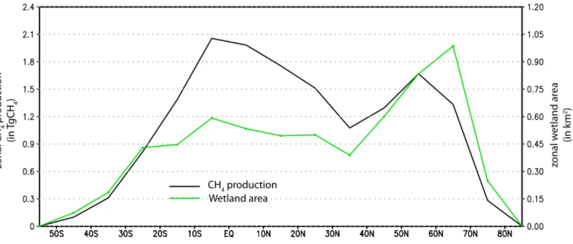
The calculated maximum global wetland extent for the PIH occurs in June and is 6.3×106km2. During minimum inundation, which occurs in December, the total wet-land area is 3.6×106km2. Taking into account that PIH wetlands were possibly ∼20% larger than today due to destruction by agriculture (Chappellaz et al., 1993),

5

this agrees with contemporary estimates based on satellite data of 5.9×106km2 and 2.1×106km2, respectively (Prigent et al., 2007). Boreal wetlands (annual average) make out 38% of the global annual mean, which is consistent with estimates for the present (Lehner and D ¨oll, 2004; Prigent et al., 2007). Simulated wetland extent peaks in high northern latitudes (45◦_N–65◦_{N), while extensive wetlands are also found in the}

10

tropics (Fig. 1).

Total simulated annual emissions amount to 151 Tg CH4, of which 35 Tg (23%)

orig-inates in boreal wetlands and 116 Tg (77%) in the tropics. This distribution is in agree-ment with many previous observational and modeling studies, which find that 15–37% of the global emissions comes from boreal wetlands and 56–85% originates in tropical

15

wetlands (Cao et al., 1996; Walter et al., 2001; Valdes et al., 2005). Boreal wetland area peaks during early summer when snowmelt rates surge, but the average tem-perature is still low (Fig. 2). Together with the limited emission season this makes the higher latitudes a less e_fficient source of CH₄ than the tropics. Therefore, the peak in simulated wetland extent in the high latitudes only translates in a moderate level of

20

emissions (Fig. 1).

Global wetland area during the LGM is at its maximum in June with 5.3×106km2 and at its minimum in December with 3.3×106km2, a decrease of 17% in the annual-mean compared to the PIH. Boreal wetlands make up∼26% of the annual global mean, shifting the main component of wetland extent towards the tropics. This change of

dis-25

(10)

CPD

7, 47–77, 2011

Title Page

Tables Figures

◭ ◮

Back Close

Full Screen / Esc

Discussion

P

a

per

|

Dis

cussion

P

a

per

|

Discussion

P

a

per

|

Discussio

n

P

a

per

|

118 Tg CH₄/yr (21%). Tropical emissions are reduced by 12%, while boreal emissions drop by 58%. Previous GCM-based modeling studies have found similar moderate re-ductions in global emissions of 16–29% (Kaplan, 2002; Valdes et al., 2005; Kaplan et al., 2006) as well as stronger reductions of 29–42% (Weber et al., 2010).

A large cooling occurs in higher latitudes during the LGM. For example, Wu et

5

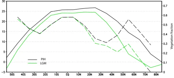
al. (2007) reconstructed a 10◦C surface cooling in the Northern Hemisphere (NH), while only minor to moderate cooling takes place in the tropics: 0–3◦C. This is accu-rately simulated by CLIMBER-2 (Fig. 3). The strong cooling of the boreal zone limits the ability of large areas to sustain wetlands during most of the year due to the tem-perature constraint (Sect. 2.2). This temtem-perature-effect is larger than the direct loss

10

of wetland area by ice cover. Additionally, the decreasing temperature has a negative impact on vegetation growth. Figure 3 shows that vegetation cover was strongly dimin-ished in the LGM with respect to the PIH in boreal latitudes, while there is little change in the tropics.

3 Main sources and controls of wetland methane emissions

15

3.1 Simulated emissions in the transient run

Figure 4 shows timeseries of the forcings used in the transient run, namely ice vol-ume, greenhouse gas variations and insolation at 65◦N as an illustration of the orbital forcing. We also show the global mean values of the main climatic parameters, as derived from CLIMBER-2, determining wetland CH4emissions, wetland extent and the

20

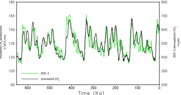
emission temperature (average temperature over grid cells emitting CH₄), as well as the vegetation cover. All parameters show variations on multiple (orbital) timescales. Simulated temperature and vegetation changes, together with the varying wetland dis-tribution, were used to compute total annual and global CH₄ emissions. These were found to vary between 116 and 167 Tg/yr. In Fig. 5 the global CH₄emissions are

com-25

(11)

CPD

7, 47–77, 2011

Title Page

Tables Figures

◭ ◮

Back Close

Full Screen / Esc

Discussion

P

a

per

|

Dis

cussion

P

a

per

|

Discussion

P

a

per

|

Discussio

n

P

a

per

|

shows pronounced sub-orbital variability, which is absent from the simulated curve. This is because CLIMBER-2 lacks internally-generated variations on these timescales. Simulated climate and vegetation are driven by the applied forcings, which vary on or-bital timescales. The longer-timescale variations (>3 kyr) in both curves correspond very well (r=0.79).

5

As wetlands are the main natural source, wetland CH4emissions for a large part

de-termine atmospheric concentrations during this period. Therefore we directly compare measured concentrations and simulated wetland emissions here. Spectra of the two time series were determined using Analyseries (Pailliard et al., 1996). Both spectra (Fig. 6) indicate a strong 100 kyr signal and significant influence of 41 kyr oscillations.

10

Precession related features (i.e. 23 kyr) show a stronger signal in the model results than in the measured data. However, differences in the relative importance of spec-tral peaks in measured concentrations and simulated global emissions could be due to lifetime variations that cannot be accounted for in the present model set-up. The atmospheric CH4lifetime was tentatively diagnosed from the measured concentrations

15

and simulated total wetland emissions. Assuming a constant biomass burning source of 40 Tg CH₄/yr (Fisher et al., 2008) and additional covarying sources, like ruminants, termites and geological sources, amounting to 30 Tg CH4/yr during the PIH (Denman

et al., 2007), we find that lifetimes vary between∼5.5 year during periods of low CH4

concentrations, and ∼9 year during periods of high CH4 concentrations. These are

20

reasonable values, which support our conclusion of close correspondence between the measured and simulated timeseries.

In order to further analyze the origin of simulated wetland emissions we separately consider three regions (Fig. 7): the areas influenced by the I/A summer monsoon, the boreal area north of 30◦N, but excluding the East Asian monsoon grid box, and the

25

tropical area, 30◦_S–30◦_{N, excluding the remaining monsoon-dominated grid boxes.}

(12)

CPD

7, 47–77, 2011

Title Page

Tables Figures

◭ ◮

Back Close

Full Screen / Esc

Discussion

P

a

per

|

Dis

cussion

P

a

per

|

Discussion

P

a

per

|

Discussio

n

P

a

per

|

Intertropical Convergence Zone (ITCZ) determine whether wetlands can exist or not. The bulk of global emissions (72% during the PIH) are emitted from the tropics. The boreal zone and the monsoon areas contribute the remainder (18% and 9% respec-tively). The spectra for the individual regions (Fig. 6) show that they each have a typical timescale behavior, as mentioned above. Emissions from the I/A monsoon

5

area are primarily controlled by precession, with little to no influence from 100 kyr and 41 kyr. Boreal emissions mainly reflect 41 kyr and 100 kyr signals, while tropical emis-sions contain a strong precession signal and significant power at the 41 kyr and 100 kyr frequencies.

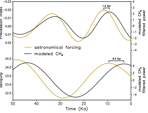
The EDC-3 record for CH₄and the time series for simulated global emissions, as well

10

as those of the separate regions, were band pass filtered using Analyseries (Pailliard et al., 1996) at 21 (±2.5) kyr and 41 (±3.5) kyr. The filtered signals were then cross correlated to the astronomical precession index and obliquity parameter, respectively (Laskar, 2004). The measured EDC-3 derived methane concentration is found to lag the orbital forcing by 2.0 kyr on the precession timescale and by 5.5 kyr on the obliquity

15

timescale (Table 1). For the simulated global emissions lags are 1.3 kyr and 5.3 kyr, respectively, (Fig. 8). We consider this a very close match given that climate models are generally not successful in reproducing lags found in measured data (e.g. Ziegler et al., 2010). Lags are longest for emissions from the boreal zone and smallest for emissions from the monsoon areas, with intermediate lags for tropical emissions (Table 1).

20

3.2 Factor analyses

The next step is to analyze the climate and vegetation factors that control variations in simulated CH4 emissions and the simulated lags. First we define a total modification

factorF_tot as follows:

Ftot(t) = E(t)/EPIH (3)

25

whereEdenotes annual emissions,tis time andEPIHdenotes annual emissions during

(13)

CPD

7, 47–77, 2011

Title Page

Tables Figures

◭ ◮

Back Close

Full Screen / Esc

Discussion

P

a

per

|

Dis

cussion

P

a

per

|

Discussion

P

a

per

|

Discussio

n

P

a

per

|

emission changes, namely changes in wetland cover (Fc), in vegetation cover (Fv) and

in temperature (Ft). To compute individual modification factors for each grid box, one

term in Eq. (2) was set at its transient value and the other two terms were set at PIH values. The results were then divided by the emissions of that grid box for the PIH. Equation (5) shows this factorial calculation for wetland cover (Fc):

5

Fc(t) = k × C(t) × VPIH × Q

T/10

10,PIE/EPIH (4)

wherek is the unaltered tunable constant, C(t) is the transient wetland cover, VPIH is

the vegetation cover and QT/₁₀_,10_PIH is the temperature dependence, both fixed at their PIH values. For each grid box Ftot is equal toFc×Fv×Ft. The results from the factor

analysis are averaged globally and for the three separate zones defined above using a

10

weighted average. By weighing the modification factors of each grid box according to their PIH emissions in the averaging process, skewing effects of extreme modifications in low-emission cells such as in high boreal latitudes are countered.

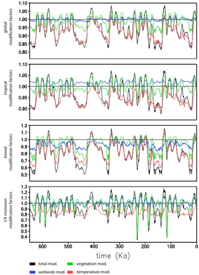
Timeseries of the modification factors (Fig. 9) show that temperature is the dom-inant control both for tropical and boreal emissions, with vegetation as a secondary

15

role. During cold periods wetland extent is a reducing factor in the boreal zone, but an amplifying factor in the tropics, possibly related to reduced evaporation. However, the effect is small in both zones and almost cancels out in the global mean. Wetlands cov-erage is only an important factor in the I/A monsoon region, together with vegetation changes.

20

Spectral analyses (Fig. 10) show that precession-related variability is dominated by vegetation changes in the tropics and in the I/A monsoon region, while in the boreal zone a combination of temperature and vegetation changes play a role. This results in global emissions dominated by vegetation at the precession timescale, with a smaller impact from temperature. At the obliquity timescale temperature and vegetation are

25

(14)

CPD

7, 47–77, 2011

Title Page

Tables Figures

◭ ◮

Back Close

Full Screen / Esc

Discussion

P

a

per

|

Dis

cussion

P

a

per

|

Discussion

P

a

per

|

Discussio

n

P

a

per

|

present in all three zones.

To summarize, at the precession timescale vegetation is the dominant control of global methane emissions, with temperature as a secondary control. The dominance of vegetation control originates primarily from the tropics. There is also a clear impact of vegetation in the I/A monsoon area, but these constitute only a small part of the

5

global emissions. At the obliquity timescale temperature and vegetation play equally important roles. The temperature changes are almost completely in phase with ice volume minima/greenhouse gas maxima. Vegetation changes lag summer insolation maxima by ca. 1kyr for precession to 2–4 kyr for obliquity (Table 1). This reflects the strong influence of hydrological processes, which respond quasi-instantaneously

10

to the orbital forcing, on vegetation. For both temperature and vegetation lags tend to be longer in the boreal zone than in the tropics (Table 1). The combined effect of temperature and vegetation, explains the lags that are found between simulated methane emissions and the orbital forcings.

4 Summary, discussion and conclusions

15

We have simulated wetland CH4 emissions over the last 650 000 yrs using a simple

wetland distribution and CH₄ emissions model coupled off-line to the atmosphere-ocean-vegetation climate model CLIMBER-2. The resulting simulated global emissions show a close similarity to the measured EDC-3 timeseries of atmospheric CH4

concen-trations, both in spectra and in lags with respect to the orbital forcing. Diagnosed CH₄

20

lifetimes vary between∼5.5 and 9 yr on glacial-interglacial timescales, with 8.2 yrs as estimated for the PIH. This is consistent with data (Fisher et al., 2008) and model studies that include atmospheric chemistry (Lelieveld et al., 1998).

Global emissions are dominated by emissions from the tropics. However, in contrast to the general assertion that monsoon intensity is of primary importance (Chappellaz

25

(15)

CPD

7, 47–77, 2011

Title Page

Tables Figures

◭ ◮

Back Close

Full Screen / Esc

Discussion

P

a

per

|

Dis

cussion

P

a

per

|

Discussion

P

a

per

|

Discussio

n

P

a

per

|

to global emissions. As hypothesized by Crowley (1999), monsoon precipitation and global emissions do co-vary, but there is no causal link. For the remainder of the trop-ics, wetland extent exerts little control on emissions. Tropical temperature variations are found to be small, about 2–4◦C on glacial-interglacial timescales in agreement with proxy data (Farrera et al., 1999). However, such variations are significant as

methano-5

genesis is much more sensitive to temperature changes at the high average tempera-tures in the tropics than at the lower average temperatempera-tures at high latitudes (compare Eq. 2).

The present results show that temperature and vegetation are the dominant controls of orbital-scale variations in global wetland CH₄ emissions, while wetland extent plays

10

a minor role. This is supported by a recent modeling study, based on an eight-member ensemble of GCM simulations for the LGM, which also found temperature and vege-tation as the main controlling factors (Weber et al., 2010). In the latter study wetlands exhibited southward shifts in the cold LGM climate, related to a southward shift of the mid-latitude storm tracks and the ITCZ. This caused the effect of changes in wetland

15

distribution to cancel out in the global mean. Here we find a shift from the boreal to the tropical zone. This larger-scale pattern is likely related to the coarse resolution of CLIMBER-2 and the fact that the atmospheric dynamics are simplified, so that storm tracks are not resolved. This is a shortcoming of the present simulation. However, it does not seem to a_ffect our main conclusion on the primary role of temperature and

20

vegetation.

Orbital cycles in vegetation have been found in many studies based on pollen data, for example for tropical South America (Hooghiemstra et al., 1993), Southeast Asia (Tsukada, 1996), Europe (Tzedakis et al., 2009) and North America (Whitlock and Bartlein, 1997). These studies indicate large shifts in vegetation presence and cover

25

(16)

CPD

7, 47–77, 2011

Title Page

Tables Figures

◭ ◮

Back Close

Full Screen / Esc

Discussion

P

a

per

|

Dis

cussion

P

a

per

|

Discussion

P

a

per

|

Discussio

n

P

a

per

|

Finally, our results provide a plausible explanation for the lags found in the measured EDC-3 curve with respect to the orbital forcing. Atmospheric CH₄concentrations have previously been related to monsoon precipitation (Ruddiman and Raymo, 2003). Here we find that lags in the CH4record are very likely due to temperature and vegetation

e_ffects rather than monsoon precipitation. The former two factors have a phasing

in-5

between insolation maxima and ice sheet/greenhouse gas minima. This results in lags that are very close to those found in measured CH4 data, both at the precession and

obliquity timescale. In contrast, simulated monsoon precipitation has zero lag at the precession band (Weber and Tuenter, 2011). This is inconsistent with any proxy-based estimate, as proxy records which have been interpreted as reflecting Indian/Asian

sum-10

mer monsoons have been found to lag precession by lags varying from 3 kyr (Wang et al., 2008) to considerably longer lags of up to 8 kyr (Clemens and Prell, 2003). Process-based modeling of proxies seems a necessary step to substantiate a reinterpretation of proxy records (Ziegler et al., 2010; Clemens et al., 2010) and to resolve this mismatch among different proxy data as well as between simulated and measured records.

15

References

Bintanja, R., van de Wal, R. S. W., and Oerlemans, J.: Modelled atmospheric temperatures and global sea levels over the past million years, Nature, 437, 125–128, 2005.

Blunier, T., Chappellaz, J., Schwander, J., Stauffer, B., and Raynaud, D.: Variations in atmo-spheric methane concentration during the Holocene epoch, Nature, 374, 46–49, 1995.

20

Braconnot, P., Otto-Bliesner, B., Harrison, S., Joussaume, S., Peterchmitt, J.-Y., Abe-Ouchi, A., Crucifix, M., Driesschaert, E., Fichefet, Th., Hewitt, C. D., Kageyama, M., Kitoh, A., Laˆın ´e, A., Loutre, M.-F., Marti, O., Merkel, U., Ramstein, G., Valdes, P., Weber, S. L., Yu, Y., and Zhao, Y.: Results of PMIP2 coupled simulations of the MidHolocene and Last Glacial Maximum -Part 1: experiments and large-scale features, Clim. Past, 3, 261–277,

doi:10.5194/cp-3-261-25

2007, 2007.

(17)

CPD

7, 47–77, 2011

Title Page

Tables Figures

◭ ◮

Back Close

Full Screen / Esc

Discussion

P

a

per

|

Dis

cussion

P

a

per

|

Discussion

P

a

per

|

Discussio

n

P

a

per

|

Cao, M., Marshall, S., and Gregson, K.: Global carbon exchange and methane emissions from natural wetlands: Application of a process-based model, J. Geophys. Res., 101, 14399– 14414, 1996.

Chappellaz, J., Barnola, J. M., Raynaud, D., Korotkevich, Y. S., and Lorius, C.: Ice-core record of atmospheric methane over the past 160,000 years, Nature, 345, 127–131, 1990.

5

Chappellaz, J. A., Fung, I. Y., and Thompson, A.M., The atmospheric CH₄ increase since the Last Glacial Maximum, 1. Source estimates, Tellus B, 45, 228–241, 1993.

Chen, Y. and Prinn, R. G.: Estimation of atmospheric methane emissions between 1996 and 2001 using a three-dimensional global chemical transport model, J. Geophys. Res., 111, D10307, doi:10.1029/2005JD006058, 2006.

10

Christensen, T. R., Ekberg, A., Strom, L., Mastepanov, M., Panikov, N., Oquist, M., Sven-son, B. H., Nykanen, H., Martikainen, P. J., and OskarsSven-son, H.: Factors controlling large scale variations in methane emissions from wetlands, Geophys. Res. Lett., 30(7), 1414, doi:2003GL016848, 2003.

Clemens, S. C., Prell, W. L., and Sun, Y.: Orbital-scale timing and mechanisms driving Late

15

Pleistocene Indo-Asian summer monsoons: reinterpreting cave speleotherm δ18O, Paleo-ceanography, 25, PA4207, doi:10.1029/2010PA001926, 2010.

Crowley, T. J.: Ice-age methane variations, Nature, 353, 122–123, 1991.

Denman, K. L., Brasseur, G., Chidthaisong, A., Ciais, P., Cox, P. M., Dickinson, R. E., Hauglus-taine, D., Heinze, C., Holland, E., Jacob, D., Lohmann, U., Ramachandran, S., da Silva Dias,

20

P. L., Wofsy, S. C., and Zhang, X.: Couplings Between Changes in the Climate System and Biogeochemistry. In: Climate Change 2007: The Physical Science Basis. Contribution of Working Group I to the Fourth Assessment Report of the Intergovernmental Panel on Cli-mate Change, edited by: Solomon, S., Qin, D., Manning, M., Chen, Z., Marquis, M., Averyt, K. B., Tignor, M., and Miller, H. L., Cambridge University Press, Cambridge, UK and New

25

York, NY, USA, 2007

Fischer, H., Behrens, M., Bock, M., Richter, U., Schmitt, J., Loulergue, L., Chappellaz, J., Spahni, R., Blunier, T., Leuenberger, M., and Stocker, T. F.: Changing boreal methane sources and constant biomass burning during the last termination, Nature, 452, 864–867, 2008.

30

(18)

CPD

7, 47–77, 2011

Title Page

Tables Figures

◭ ◮

Back Close

Full Screen / Esc

Discussion

P

a

per

|

Dis

cussion

P

a

per

|

Discussion

P

a

per

|

Discussio

n

P

a

per

|

Gedney, N., Cox, P. M., and Huntingford, C.: Climate feedback from wetland methane emis-sions, Geophys. Res. Lett., 31, L20503, doi:10.1029/2004GL020919, 2004.

Hooghiemstra, H., Melice, J. L., Berger, A., and Shackleton, N. J.: Frequency spectra and paleoclimatic variability of the high-resolution 30–1450 ka Funza I pollen record (Eastern Cordillera, Colombia), Quaternary Sci. Rev., 12(2), 141–156, 1993.

5

Houweling, S., Dentener, F., and Lelieveld, J.: Simulation of preindustrial atmospheric methane to constrain the global source strength of natural wetlands, J. Geophys. Res., 105, 243–255, 2000.

Kaplan, J. O.: Wetlands at the Last Glacial Maximum: Distribution and methane emissions, Geophys. Res. Lett., 29, 6, 2002.

10

Kaplan, J. O., Folberth, G., and Hauglustaine, D. A.: Role of methane and biogenic volatile organic compound sources in late glacial and Holocene fluctuations of atmospheric methane concentrations, Global Biogeochem. Cy., 20, 16, 2006.

Kutzbach, J. E., Liu, X., Liu, Z., and Chen, G.: Simulation of the evolutionary response of global summer monsoons to orbital forcing over the past 280,000 years, Clim. Dynam. 30(6),

15

567–579, 2008.

Laskar, J., Robutel, P., Joutel, F., Gastineau, M., Correia, A. C. M., and Levrard, B.: A long-term numerical solution for the insolation quantities of the Earth, Astron. Astrophys., 428, 261–285, 2004.

Lelieveld, J., Crutzen, P., and Dentener, F. J.: Changing concentration, lifetime and climate

20

forcing of atmospheric methane, Tellus B, 50, 128–150, 1998.

Lisiecki, L. and Raymo, M.: A Pliocene-Pleistocene stack of 57 globally distributed benthic

δ18O records, Paleoceanography, 20, PA1003, doi:10.1029/2004PA001071, 2005.

Loulergue, L., Parrenin, F., Blunier, T., Barnola, J.-M., Spahni, R., Schilt, A., Raisbeck, G., and Chappellaz, J.: Orbital and millennial-scale features of atmospheric CH₄over the past

25

800,000 years, Nature, 453, 383–386, 2008.

L ¨uthi, D., Floch, M. L., Bereiter, B., Blunier, T., Barnola, J. M., Siegenthaler, U., Raynaud, D., Jouzel, J., Fischer, H., Kawamura, K., and Stocker, T. F.: High-resolution carbon dioxide concentration record 650 000–800 000 years before present, Nature, 453, 379–382, 2008. Peltier, W. R.: Global glacial isostasy and the surface of the ice-age Earth: The ICE-5G (VM2)

30

model and GRACE, Annu. Rev. Earth Pl. Sc., 32, 111–149, 2004.

(19)

CPD

7, 47–77, 2011

Title Page

Tables Figures

◭ ◮

Back Close

Full Screen / Esc

Discussion

P

a

per

|

Dis

cussion

P

a

per

|

Discussion

P

a

per

|

Discussio

n

P

a

per

|

description and performance for present climate, Clim. Dynam., 16, 1–17, 2000.

Prigent, C., Papa, F., Aires, F., Rossow, W. B., and Matthews, E.: Global inundation dynamics inferred from multiple satellite observations, 1993–2000, J. Geophys. Res., 112, D12107, doi:10.1029/2006JD007847, 2007.

Rice, A. L., Butenhoff, C. L., Shearer, M. J., Teama, D., Rosenstiel, T. N., and Khalil, M. A. K.:

5

Emissions of anaerobically produced methane by trees, Geophys. Res. Lett., 37, L03807, doi:10.1029/2009GL041565, 2010.

Ruddiman, W. F. and Raymo, M. E.: A methane-based time scale for Vostok ice, Quaternary Sci. Rev., 22, 141–155, 2003.

Schmidt, G. A., Shindell, D. T., and Harder, S.: A note on the relationship between

10

ice core methane concentrations and insolation, Geophys. Res. Lett., 31, L23206, doi:10.1029/2004GL021083, 2004.

Schneider von Deimling, T., Held, H., Ganopolski, A., and Rahmstorf, S.: Climate sensitivity estimated from ensemble simulations of glacial climate, Clim. Dynam., 27, 149–163, 2006. Segers, R.: Methane production and methane consumption: a review of processes underlying

15

wetland methane fluxes, Biogeochemistry, 41, 23–51, 1998.

Spahni, R., Chappellaz, J., Stocker, T. F., Loulergue, L., Hausammann, G., Kawamura, K., Flckiger, J., Schwander, J., Raynaud, D., Masson-Delmotte, V., and Jouzel, J.: Atmospheric Methane and Nitrous Oxide of the Late Pleistocene from Antarctic Ice Cores, Science, 310, 1317–1321, 2005.

20

Tsukada, M.: Late Pleistocene vegetation and climate in Taiwan (Formosa), P. Natl. Acad. Sci., 55, 543–548, 1966.

Tzedakis, P. C., Palike, H., Roucoux, K. H., and de Abreu, L.: Atmospheric methane, southern European vegetation and low-mid latitude links on orbital and millennial timescales, Earth Planet. Sc. Lett., 277(3–4), 307–317, 2009

25

Valdes, P. J., Beerling, D. J., and Johnson, C. E.: The ice age methane budget, Geophys. Res. Lett., 32, L02704, doi:10.1029/2004GL021004, 2005.

Walter, B. P., Heimann, M., and Matthews, E.: Modeling modern methane emissions from natural wetlands: 1. Model description and results, J. Geophys. Res., 106, 189–234, 2001. Wang, W.-C., Yung, Y. L., Lacis, A. A., Mo, T., and Hansen, J. E.: Greenhouse effects due to

30

man-made perturbations of trace gases, Science, 194, 685–690, 1996.

(20)

CPD

7, 47–77, 2011

Title Page

Tables Figures

◭ ◮

Back Close

Full Screen / Esc

Discussion

P

a

per

|

Dis

cussion

P

a

per

|

Discussion

P

a

per

|

Discussio

n

P

a

per

|

224,000 years, Nature, 451, 1090–1093, 2008.

Weber, S. L., Drury, A. J., Toonen, W. H. J., and van Weele, M.: Wetland methane emissions during the Last Glacial Maximum estimated from PMIP2 simulations: Climate, vegetation, and geographic controls, J. Geophys. Res., 115, DO6111, doi: 10.1029/2009JD012110, 2010.

5

Weber, S. L. and Tuenter, E.: The impact of varying ice sheets and greenhouse gases on the intensity and timing of boreal summer monsoons, Quaternary Sci. Rev., in press, 2010. Whitlock, C. and Bartlein, P. J.: Vegetation and climate change in northwest America during the

past 125 kyr, Nature, 388, 57–61, 1997.

Wu, H., Guiot, J., Brewer, S., and Guo, Z.: Climatic changes in Eurasia and Africa at the

10

Last Glacial Maximum and mid-Holocene: Reconstruction from pollen data using inverse vegetation modeling, Clim. Dynam., 29, 211–229, 2007.

Ziegler, M., Lourens, L. J., Tuenter, E., Hilgen, F., Reichart, G.-J., and Weber, S. L.:

Pre-cession phasing offset between Indian summer monsoon and Arabian Sea

productiv-ity linked to changes in Atlantic overturning circulation, Paleoceanography, 25, PA3213,

15

(21)

CPD

7, 47–77, 2011

Title Page

Tables Figures

◭ ◮

Back Close

Full Screen / Esc

Discussion

P

a

per

|

Dis

cussion

P

a

per

|

Discussion

P

a

per

|

Discussio

n

P

a

per

|

Table 1. Lags with respect to the orbital forcing in ice cover, greenhouse gases and EDC-3

atmospheric CH₄, in the TRENCH simulated global and regional emissions and in the global modification factors. Lags are computed by searching for the optimum correlation between the forcing (precession or obliquity) and a given variable, band pass filtered at 21 kyr or 41 kyr, respectively. Zero phase is set at minimum precession and maximum obliquity, which each correspond to an insolation maximum for the NH. The correlation value is displayed next to the lag.

factor precession Correlation obliquity Correlation

Ice cover 4.7 ₋0.86 7.1 ₋0.94

GHG – – 6.0 0.91

EDC-3 2.0 0.78 5.5 0.95

global emissions 1.3 0.93 5.3 0.96

boreal emissions 2.5 0.88 6.3 0.97

tropical emissions 0.7 0.95 4.4 0.96

Indian/Asian monsoon emissions 0.5 0.95 2.6 0.96

Global modification factor 1.1 0.94 4.7 0.97

Global wetland modification factor 2.1 0.88 3.2 0.95

Global vegetation modification factor 0.5 0.94 3.2 0.97

(22)

CPD

7, 47–77, 2011

Title Page

Tables Figures

◭ ◮

Back Close

Full Screen / Esc

Discussion

P

a

per

|

Dis

cussion

P

a

per

|

Discussion

P

a

per

|

Discussio

n

P

a

per

|

zonal CH

4

pr

oduc

tion

(in

TgCH

4

)

zonal w

etland ar

ea

(in k

m

2)

CH₄ production Wetland area

Fig. 1.TRENCH simulated PIH wetlands during the month of maximum wetland extent (green

(23)

CPD

7, 47–77, 2011

Title Page

Tables Figures

◭ ◮

Back Close

Full Screen / Esc

Discussion

P

a

per

|

Dis

cussion

P

a

per

|

Discussion

P

a

per

|

Discussio

n

P

a

per

|

Fig. 2.Seasonal variation of high (55–75◦N) latitude boreal wetland extent (black line) and soil

(24)

CPD

7, 47–77, 2011

Title Page

Tables Figures

◭ ◮

Back Close

Full Screen / Esc

Discussion

P

a

per

|

Dis

cussion

P

a

per

|

Discussion

P

a

per

|

Discussio

n

P

a

per

|

a

v

er

age sur

fac

e t

emper

a

tur

e

(ºC

)

V

egeta

tion fr

ac

tion

PIH LGM

Fig. 3. CLIMBER-2 simulated PIH temperature (solid black line) and LGM temperature (solid

(25)

CPD

7, 47–77, 2011

Title Page

Tables Figures

◭ ◮

Back Close

Full Screen / Esc

Discussion

P

a

per

|

Dis

cussion

P

a

per

|

Discussion

P

a

per

|

Discussio

n

P

a

per

|

Ic

e v

olume

in m of sea lev

el eq

rela

tiv

e t

o pr

esen

t

65ºN June insola

tion

in

W/m

2

Global w

etlands

annual a

ver

age

in 10

6 k

m

2

emission t

emper

a

tur

es

global annual a

ver

age

in ºC

GHG c

onc

en

tr

a

tion

stacked gobal GHG in C O2

(ppm

v) eq

v

egeta

tion fac

tor

a

ver

aged globally

Fig. 4. Transient forcings (top graphs) for CLIMBER-2 and the resulting wetland extent,

(26)

CPD

7, 47–77, 2011

Title Page

Tables Figures

◭ ◮

Back Close

Full Screen / Esc

Discussion

P

a

per

|

Dis

cussion

P

a

per

|

Discussion

P

a

per

|

Discussio

n

P

a

per

|

modeled CH

4

pr

oduc

tion

in

TgCH

4

/y

ear

EDC-3 a

tmospher

ic CH

4

in ppb

v

simulated CH4

EDC-3

Fig. 5.Epica Dome C atmospheric CH₄concentrations (green line; in ppbv), low pass filtered

(27)

CPD

7, 47–77, 2011

Title Page

Tables Figures

◭ ◮

Back Close

Full Screen / Esc

Discussion

P

a

per

|

Dis

cussion

P

a

per

|

Discussion

P

a

per

|

Discussio

n

P

a

per

|

EDC-3 simulated CH4

100K yr

41K yr

23K yr

(18K yr)

P

o

w

er in simula

ted CH

4

x10

3

P

o

w

er in EDC-3 x10

5

P

o

w

er

18K yr 23K

yr

41K yr 100K

yr _{I/A monsoon emissions}

tropical emissions boreal emissions

Fig. 6. Left: Spectra for the Epica Dome C atmospheric CH₄concentrations (green line) and

(28)

CPD

7, 47–77, 2011

Title Page

Tables Figures

◭ ◮

Back Close

Full Screen / Esc

Discussion

P

a

per

|

Dis

cussion

P

a

per

|

Discussion

P

a

per

|

Discussio

n

P

a

per

|

tropical zone

boreal zone

Indian/Asian monsoon areas

Fig. 7. Definition of the tropical (red), boreal (blue) and Indian/Asian monsoon (pink) zones.

(29)

CPD

7, 47–77, 2011

Title Page

Tables Figures

◭ ◮

Back Close

Full Screen / Esc

Discussion

P

a

per

|

Dis

cussion

P

a

per

|

Discussion

P

a

per

|

Discussio

n

P

a

per

|

Fig. 8. Top: TRENCH simulated global CH₄emissions, band pass filtered for 21 kyr (_±2.5 kyr)

(30)

CPD

7, 47–77, 2011

Title Page

Tables Figures

◭ ◮

Back Close

Full Screen / Esc

Discussion

P

a

per

|

Dis

cussion

P

a

per

|

Discussion

P

a

per

|

Discussio

n

P

a

per

|

total mod. vegetation mod. wetlands mod. temperature mod.

global

modifica

tion fac

tors

tr

opical

modifica

tion fac

tors

bor

eal

modifica

tion fac

tors

I/A monsoon

modifica

tion fac

tors

Fig. 9. Time series of the modification factors, as defined in Sect. 3.2, for the entire globe and

(31)

CPD

7, 47–77, 2011

Title Page

Tables Figures

◭ ◮

Back Close

Full Screen / Esc

Discussion

P

a

per

|

Dis

cussion

P

a

per

|

Discussion

P

a

per

|

Discussio

n

P

a

per

|

total mod. vegetation mod.

wetlands mod. temperature mod.

Global modification factors

tropical modification factors I/A monsoon modification factors boreal modification factors

Fig. 10. Spectra of the modification factors (see Sect. 3.2) for the entire globe, and for the