Vol-7, Special Issue3-April, 2016, pp896-904 http://www.bipublication.com
Case Report
Performance of Chaos Theory in Weather Forecasts
(Case Study: Tehran-Temperate Climate)
Mitra Mesbahzadeh 1, SohrabHajjam 2 and Abdullah Sedaghatkerdar 3 1Master’s Student, Islamic Azad University-
Science and Research Branch of Tehran
2 Associate Professor, Islamic Azad University-
Science and Research Branch
3Associate Professor,
Atmospheric Science & Meteorological Research Center, Tehran
*Corresponding author: Email: mitra.m2654@gmail.com
ABSTRACT:
Accurate weather forecast is of great importance for providing the suitable substrates for water resources management and crisis management. Therefore, the use of methods with high accuracy and updating the forecast models seem to be necessary in this regard. In evaluation of hydrological and climate data, the investigation of precipitation parameter is in non-linear time series method. The present research aimed to compare the performance of intelligent systems based on nonlinear methods, chaos theory, and neural network system in estimating monthly precipitation in temperate climate of Tehran. The results of neural network system, local model methods, and the nearest neighbor showed that chaos-based methods not only are sensitive to the range of data but also influenced by the length of data and attitude towards data review process based on conditions. Evaluation of results indicated that chaos-based have an acceptable and high precision and accuracy and chaos theory produces better results than neural network system in temperate climates. Considering the nature of data, the studied climate, and the procedures required in forecast of meteorological parameters, chaos theory can bring very good results. Due to the sensitivity of meteorological forecasts, the use of this theory can be helpful and beneficial.
Keywords: Chaos theory,Neural network system, Anfis ,nearest neighbor, Meteorological parameters
I NTRODUCTION
Fluctuations and distribution of studies variables are of special importance in meteorological forecasts. Climate variability itself causes different behaviors of a variable over time. This increases the need for accurate forecasts in order to provide the suitable substrates for water resources management and crisis management. In this regard, the use of methods with high accuracy and updating the forecast models seem to be necessary. On the other hand, conceptual models are dependent on several variables during their development process. This causes difficulties in model calibration considering the study
controversial. The present research aimed to propose some predictions for these indictors on the next periods by reviewing the changes in time series with a different approach and forecast based on chaos theory and also to compare the results with those obtained from neural network system in the studied area in the same period.
1.1. Chaos theory
Chaos theory deals with the study of systems that appear to have random behavior but yet follow some certain rules. In other words, regularity lies beneath any irregularity. This system is very sensitive to initial conditions and data with different accuracy and slight difference will show a great impact on the system. This high sensitivity is referred to as the butterfly effect in the world of science (does theflap of a butterfly’s wings in Brazil set off a tornado in Texas?). Minor changes in initial conditions can lead to unexpected and widespread results. Such a system is known as chaotic system. Instability, non-periodic behaviors, absolute systems, and non-linearity are characteristics of a chaotic system [12].as regardsLimited hydrological data can show chaotic behavior [16].Chaos theory introduced the butterfly effect with the research of Edward Lorenz (1963) who applied the fractal effects observed for differential equations model of convection in the fluid layer to a meteorological model and introduced it to the natural system analysis field [7,21]. Alttikallioet al. (1999) proposed a new method for estimation of low degrees of chaos by studying the false nearest neighbor (FNN) algorithm. Wang (1998) and Krasuskaya (1999) studied chaotic behavior in a time series in the natural system of a river flow. The found that the use of models based on chaos theory requires the identification of chaos and its degree separately.Kocaket al. (2007) studied the monthly flow forecast of Yamla Dam using the local prediction model of Chaos Theory. Their findings showed that short-term forecasts had better results than other methods. Rulle (1980) studied the nature of chaotic attractions. Al-Bostan (2014) studied the non-linear trend of data
related to the catchment of YesilAyrmaq River using three techniques off correlation dimension, fuzzy space, and local model and obtained acceptable results in prediction of the chaotic behavior of this catchment. Badin (2013) studied the turbulent behavior of the stratosphere and chaotic factors in this layer of the atmosphere in different seasonal conditions. The results showed no seasonal structure of chaotic attraction. Domeisen and Badin (2014) studied the stratosphere in both northern and southern hemispheres considering some variables such as regional winds, temperature, and geo-potential height using chaos theory and obtained a limited value for each variable in a wide range. Fitton (2014) studied the fractal analysis of wind energy. Bojan (2015) studied turbulence in the atmospheric column of the ozone layer over the Arctic in an area called Svalbard and provided a short-term forecast using the fractal chaos model. Elsharbagiet al. (2002) studied the chaotic behavior of hydrologic data and the impact of noise on forecasts. Monitoring the system behavior concurrent with the gradual reduction of noise, they found that chaos in hydrologic data is highly sensitive to noise removal and applying a high level of noise removal can lead to the creation of artificial chaos in the system. They also stated that the use of raw data has a higher advantage and less noise reduction in hydrologic systems produces more favorable results. Yu et al. (2009) studied the behavior of systems with different degrees of fraction and showed that chaos theory is very successful in the analysis of these systems.
1.2. Neural network system
[9].Kurtolous and Razak (2010) studied the relationship between rainfall, water level, and flow rate in France using Neuro-Fuzzy models and confirmed the superiority of neural models [15].
Banan Khan and NejadKooraki (2012) studied the application of neural network system as a non-linear model in atmospheric sciences and its advantages and disadvantages. They stated that this model is superior over other methods because of the high capacity of input and output variables and high-capacity input variables errors [18]. Nayak (2004) used ANFIS for modeling the flow of Baytarany River in India. They also developed an artificial neural model and an autoregressive moving average model in the same basin. Their findings confirmed the better performance of ANFIS in terms of both construction and results (Hosseinpour,2011). Shiriet al. (2012) compared the neuro-fuzzy and neural network models in estimation of evaporation rate in meteorological stations of the US and found the relative accuracy of neuro-fuzzy model over neural network system[14].
MATERIALS AND METHODS
This part of the paper deals with forecast processes and their description.
2.1. Local model
One of the methods used for forecast based on fuzzy space is local model method. Assuming that the time series of a system with disorderly conduct have been formed with m dimension in the state space, a new state space can be formed by adding an additional independent coordinates. One of these independent coordinates is time series itself and other coordinates are obtained through delaying (m-1) τ against the main time series, as correlation between the coordinates becomes zero. For this time series, we have:
(1)
(2)
(3)
Xi is a m-dimensional vector of x,…,xi-(m-1)τ values. Such a trend in the structure of the state space of a system is caused by characteristics of the absorbent. Forecast is done by considering the Xi change with time. Considering the relationship between Xt and Xt+pin time p, the absorber is approximated by the function f.
(4)
It is assumed that the Xi change with time in the absorber is the same as the points in neighbor N. Xt+p( ) is determined by the Dth order of multi-function of F(Xt) [16].
(5)
Using the n number XTk and XTk+p of preset values, f coefficients are determined by the following equation.
(6)
(7)
) (8)
And A is the Jacobian matrix with the dimensions of n×(m+d)!/m!d! as follows:
(9)
It is noteworthy that even if f is a first-degree polynomial, forecast will be still non-linear, because each point of X(t) during the forecast process may have different neighbor and different expressions for f [12].
2.2. Neural network system
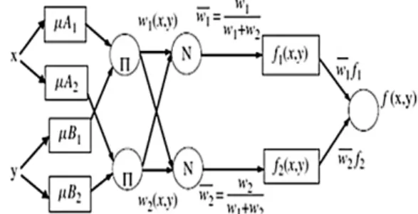
Adaptive neuro-fuzzy inference systems (ANFIS) include multi-layer network systems and use the
originally developed and introduced by Jang (1993). Due to the ability to combine the power of a fuzzy system with numerical strength of a neural network system, this system has achieved many successes in modeling and controlling of complicated systems [13].The neural network system is initially supplied with a model and then the output is calculated. Weight coefficients of network vary with the comparison of the actual output and the desired output, as a better output will result with more repetitions.
Figure 1: A schematic view of an adaptive neuro-fuzzy inference system
2.3. K-Nearest neighbors method
Algorithm K is the nearest neighbor of a supervised learning algorithm. In general, this algorithm is used for two purposes: estimation of
the density function of education data distribution and classification of test data based on education pattern. The nearest neighbor method aims to classify and estimate the characteristics of a given series of unknown data with regard to their similarities to a series of known data in their neighborhood [19].
In this method, data are classified and valued evaluated based on the obtained distances using the metering function. After selecting the best neighbor, different values of weights are considered and finally the weights with the lowest gev are selected.
(10)
Where, N denotes the number of data and e represents the forecast error. Then, K is determined.
(11)
The nearest neighbors are ranked from 1 to k. Finally, the forecast value is calculated by the following equation.
(12) D(t) is the dependent variable in time t and D(t-i) is the dependent variable in time t-i [4].
RESULTS 3.1. Study area
The city of Tehran lies at 35°41'46" N 51°25'23" E and its height from sea level is 1800 meters in north, 1200 meter in center, and 1050 meters in south.
3.2. Process of data analysis
Monthly precipitation data for 41 years in Tehran, as a moderate climate, were studied. To study the behavioral trend of statistical data, two models were selected as follows:
1- Model A: The 30-year-old data from 1947 to 2003 were allocated for education of systems and the data related to the period 2004-2014 were analyzed to test the results and assess the accuracy of forecasts. In this model, annual data are used in the forecast in a vector form considering the sequence of a year’s months.
2- Model B: Data of 30 years were separated for each month and the behavior of data was studied in each month in this period. The forecast obtained for each month was compared with the data related to the period 2004-2014.
Model B aimed to forecast the data related to the months of high rainfall and low rainfall based on figures for the same months in previous years by taking into account the different nature of rainfall in each month of the year, so that an assessment of the validity of these intelligent systems in functionality accountability to this attitude was provided.At first, data were classified using the c-means method of pre-processing and then they were analyzed.
3.3. Forecast
nearest neighbor were studied in order to assess the chaos of the system.
It is noteworthy that before providing a forecast based on chaos theory, chaotic parameters such as fuzzy space, Lyapunov power, and so on were studied and the results confirmed the chaotic nature of the studied variable in the desired period.
3.3.1. Neural network system
Model A- In this step, statistical data with Model A were used as the input of neural network system. The root-mean-square error (RMSE) of forecast of data presented by this system has been shown in Table 1.
RMSE Year
5.33 2004
4.35 2005
7.17 2006
16.41 2007
6.74 2008
13.51 2009
7.07 2010
4.08 2011
10.34 2012
10.25 2013
15.20 2014
Table 1:Forecast error of neural network system- Model A
According to above table, the lowest and the highest RMSE belong to 2011 (4.08) and 2005 (4.35), respectively. In addition, the highest error values in the period 2004-2014 are related to the forecast of monthly rainfall in 2007 (16.41) and 2014 (15.20).
Model B- In this part, statistical data were set as the input by month. The RMSE estimated in forecast results of neural network system has been presented in Table 2.
Table 2: Forecast error of neural network system- Model B
As this table shows, the lowest and the highest error rates belong to August (7.65) and September (8.93), respectively. High figures in this table are related to April (514.82), October (165.18), and January (143.38) that are remarkable.
The results indicate that Model B provides rainfall forecasts with negative figures and high error of the system. It can be argued that neural network system was not able to estimate the proper weight for forecast of data related to the high rainfall months and it has only the ability to do so for the low rainfall months.
According to the results obtained from neural network system forecast for Model A and Model B, it can be stated that neural network system has an acceptable performance in Model A and results are of good accuracy.
3.2.2. Local model
Model A: In this part, forecast by local model system was estimated using the statistical data. The RMSE estimated for monthly rainfall forecast has been shown in Table 3.
RMSE Month
RMSE Month
26.45 July
143.38 January
7.65 August
76.64 February
8.93 Septembe
r 46.03
March
165.18 October
514.82 April
50.85 Novembe
r 34.64
May
39.98 Decembe
r 21.93
Mitra Mesbahzadeh, et al. 901
Table 3: RMSE of local model in Model A
The prediction errors obtained by the system are based on e-13 degree and figures show very low
error. According to this table, the highest and the lowest RMSE belong to 2013 (6.5 e-13) and 2005 (7.1 e-13), respectively.
Very low rates of RMSE shows that this system has been successful in detection of the chaotic behavior of data related to studied stations and providing a suitable forecast model based on the existing chaotic model and results are of good accuracy.
Model B: Table 4 presents the values of RMSE related to local model in Model B in the studied period. RMSE Month RMSE Month 83.93 July 41.82 January 7.44 August 15.03 February 22462.03 September 34.96 March 11.74 October 88.52 April 47.32 November 6.74 May 16.45 December 14850.86 June
Table 4 :RMSE of local model in Model B
According to the table, the lowest rates of errors were 6.74 and 7.44 in May and August, respectively. However, the highest rates of errors were 1485.84 and 22462.03 in June and September, respectively. Given the forecast with the negative values of precipitations, it can be stated that these results are not acceptable. On the other hand, the error rates represented different dispersion amplitudes in other months, a fact which shows the extremely poor performance of the system in detecting the chaos trend of data. Comparing the results and considering the quantity type of precipitation, it can be concluded that the local model system was very successful in detecting the chaotic behavior and trend to provide appropriate forecasts for the implementation of Pattern A. The results were highly accurate. However, this system is inefficient in providing forecast forseparatemonthsand considering the nature of research data in implementation ranges.
3.3.3. k-Nearest Neighbors Algorithm (KNN) Pattern (A): In this part, the statistical data were thought of as an annual vector. The results of RMSE error pertaining to the forecasts, provided in this method, can be seen in Table 5
Table 5: The Forecast Error in knn – Pattern A
According to the table, the error rates, estimated in the study period, are almost in the same range. The highest rate of error was 23.37 in 2004, whereas the lowest error rate was 7.53 in 2006. It can be reasoned that the forecast, provided by knnSystem, presented low rate of errors and enough accuracy in pattern (A).
RMSE Year
1.27 e-13
2004
7.1 e-14
2005
2.76 e-13 2006
2.95 e-13 2007
8.29 e-14 2008
3.56 e-13 2009
1.6 e-13 2010
6.12 e-14 2011
4.65 e-13 2012
6.5 e-13 2013
Pattern (B): The error rate of rmse, estimated for the results of forecasts in pattern (B), can be seen in Table
RMSE Month
RMSE Month
4.92 July
13.17 January
7.17 August
20.80 February
2.87 September
8.38 March
14.00 October
24.00 April
5.73 November
7.78 May
16.29 December
2.60 June
Table 6: The Forecast Error in knn– Pattern B
The highest rate of error was 24.00 in April. The lowest error rates were 2.6 and 2.87 in June and September, respectively. Therefore, the results were so accurate.It can be concluded that KNN was very successful in the implementation range of pattern (B), and the results were highly accurate.Comparing the forecasts obtained in patterns (A) and (B), the performance of this forecast system was quite acceptable for both inputs annually and in separate months, and the results presented sufficient accuracy.Comparing the performances of systems indicated that the error rates of forecasts estimated by KNN system was the highest rate in the implementation range of pattern (A). The neural network system presented a mediocre performance in processing and estimating the precipitation in this climate, and the error rates were between 5 and 15. The lowest rate of errors in forecasts were provided by the local model system in e-14 range. The low rate of error, presented by the local model system, indicate the great performance of this method in comparison with previous methods in investigating the climatic data of monthly precipitation in this climate.In the research into the forecasts provided by these three methods for monthly patterns, the local model system and neural network system did not present enough accuracy and validity. The KNN had a good performance in estimating forecasts with the input
monthly pattern. Since this system is based on data classification, it could not detect data better and determine the correct neighborhood for the input data with greater ranges and higher chaos degree in the first pattern. In fact, this algorithm presented good results in short input data and low chaos degrees. This system also provided good results in responding to the hypothesis based on the forecast data pertaining to months with high and low precipitations with respect to the statistics for the same months in previous years.In the two systems introduced for chaotic data, the system input conditions were highly important. Since the evaluation pattern is chaotic, the sensitivity of forecast systems to the chaotic behavior conditions of data such as the length and range of data should also be taken into account. In systems with longer ranges of data, the proper weighting methods can be used such as the local model. Regarding short data of low ranges, the KNN can be used.It should also be mentioned that investigations were also conducted on hot, dry and humid climates by the author of the current paper. The results were different in details, and the findings of this study are merely about mild climates.
CONCLUSION
with the results of the three methods, the climatic data indicated that the chaos theory had a better performance in estimating forecasts in both annual and monthly patterns rather than the neural network system. In the annual pattern, the local model system was used; however, the KNN was used in the second pattern to analyze the statistics of mild climates.Not only are the forecasts based on chaos sensitive to data variations, but also the length of data and attitude towards the investigation would influence the results. The local model for chaotic data provided very good results in longer data pertaining to the annual pattern in the mild climate by detecting the chaotic pattern and weighting based on the chaotic situation. It had a better performance compared with the intelligent neural network system. Regarding data having shorter chaotic ranges for which the understandability of a proper weighting pattern is not possible, the methods based on the system phase space would be used to estimate parameters. The results were also highly accurate.Regarding weather forecasts and the importance of variations, length and range of variables, the chaos theory considers the variable ranges and sensitivity of results to the study conditions. The behaviors of variable were also taken into account with respect to the conditions of climate to provide more accurate and valid forecasts for meteorological systems. A proper attitude towards the study variables and climatic conditions in the forecast systems can lead to better results in the proper estimation of meteorological components.
REFERENCES
1. Aittokallio T. , Gyllenberg M. , Hietarinta J. ,(1999),” Improving the false nearest neighbors method with graphical analysis” ,Physical Review E, 60, pp,416-423
2. Alami M. T. , Ghorbani M. A. ,Malekani I. ,(2013), “ Chaotic analysis and prediction of river flow” , Scientification professional quarterly ,1, pp ,51-61
3. Albostan A. , Önöz, B.,( 2015),” Implementation of Chaotic Analysis on River Discharge Time Series”, Energy and Power Engineering ,7, pp,81-92
4. Azmi, M; Araghinejad, Sh; (2011); Developing the Regression Method of the Nearest K-Neighbor for Predicting the Flow of River; Water and Wastewater; 2; 108-119
5. Badin G. , Domeisen D.I. ,(2014), “ A search for chaotic behavior in northern hemisphere stratospheric variability”, Journal of the Atmospheric Sciences, 71, pp,1494-1507 6. Boyan .HP.., Vitale V., Mozzola M.,(2015), “
Chaotic behavior of the short-term variation in ozone column observed in Arctic”, Commun nonlinear Scinumersimult, 26, pp 238-249 7. Deidda R., (1999),”Multifractal analysis and
simulation of rainfall fields in space ,physics and chemistry of the earth part b hydrology Oceans and Atmophere”,24,pp73-78
8. Elshorbagy A., Simonovic S.P. and Panu, U.S., (2002), “ Noise reduction in chaotic hydrologic time series: facts and doubts”, Journal of Hydrology, 256, pp,147-165
9. Fattahi, M; Bidokhti, N, T; …; (2010); the Fractal Evaluation of Wavelet Forecast Method for the Time Groups of River Flow; Journal of Water Engineering; Year 3; Summer 2012; 1-11
10.Fattahi, M; Bidokhti, N, T; …; (2012); A Multi-Fractal Approach to the Time Chain of Floodwater Flow on the GhareAgh River; Journal of Water Resources Engineering; Year 5; spring 2012; 95-110
11.Fitton G., (2013),” Multifractal analysis and simulation of wind energy fluctuations” (Doctoral dissertation, Université Paris-Est) 12.Ghaheri, A; Ghorbani, M, A; … (2012); the
Evaluation of River Flow Using the Chaos Theory, Journal of Iran Water Research; Year 6; No. 10; Spring and Summer 2012; 1-10 13.Karimi, S; Shiri, J; …; (2013); the Daily
14.Karimi, V, A; HabibNejadRoshan, M; … (2010); Investigating the Meteorological Drought Index at Synoptic Stations in Mazandaran; Irrigation and Water Engineering; 15-25
15.KhasheySivki, A; Ghahreman, B; Kuchekzadeh, M; (2013); Comparing the Artificial Neural Network system, ANFIS and Regression Models in Estimating the Static Level of AbkhanDashtNeishabour; Iran Irrigation and Drainage; 7; 10-22
16.Kocak K., Bali A., Bektasoglu B.,(2007),” Prediction of Monthly Flows by Using Chaotic Approach” , In International Congress on River Basin Management, pp, 22-24
17.Ruelle D.,( 1980),” Strange attractors”, Math. Intelligencer, 2, pp,126-137.
18.Tavakoli, M; Esmaeeli Sari, A; (2014); the Performance of an Artificial Neural Network
system and an Adaptive Fuzzy Neural Network system in the Estimation of Aerosols in Tehran; Environmental Sciences and Engineering; 2; 75-84
19.Wu, X. and Kumar, V., 2009. The top ten algorithm in data mining. International Standard Book, 13, pp.978-1.
20. Yu Y., Li H., Wang S.,(2009),” Dynamic analysis of a fractional order loranz chaotic system” , chaos, solitions and fractals ,42, pp 1181-1189