www.atmos-chem-phys.net/13/10517/2013/ doi:10.5194/acp-13-10517-2013
© Author(s) 2013. CC Attribution 3.0 License.
Atmospheric
Chemistry
and Physics
Filamentary structure in chemical tracer distributions near the
subtropical jet following a wave breaking event
J. Ungermann1,2, L. L. Pan2, C. Kalicinsky3, F. Olschewski3, P. Knieling3, J. Blank1, K. Weigel4, T. Guggenmoser1, F. Stroh1, L. Hoffmann5, and M. Riese1
1Institute of Energy and Climate Research – Stratosphere (IEK-7), Research Centre Jülich GmbH, Jülich, Germany 2National Center for Atmospheric Research, Boulder, Colorado, USA
3Department of Physics, University of Wuppertal, Wuppertal, Germany
4Institute of Environmental Physics (IUP), University of Bremen, Bremen, Germany 5Jülich Supercomputing Centre, Research Centre Jülich GmbH, Jülich, Germany
Correspondence to:J. Ungermann (j.ungermann@fz-juelich.de)
Received: 29 October 2012 – Published in Atmos. Chem. Phys. Discuss.: 21 February 2013 Revised: 9 September 2013 – Accepted: 30 September 2013 – Published: 31 October 2013
Abstract.This paper presents a set of observations and anal-yses of trace gas cross sections in the extratropical upper tro-posphere/lower stratosphere (UTLS). The spatially highly re-solved (≈0.5 km vertically and 12.5 km horizontally) cross sections of ozone (O3), nitric acid (HNO3), and
peroxy-acetyl nitrate (PAN), retrieved from the measurements of the CRISTA-NF infrared limb sounder flown on the Russian M55-Geophysica, revealed intricate layer structures in the re-gion of the subtropical tropopause break. The chemical struc-ture in this region shows an intertwined stratosphere and tro-posphere. The observed filaments in all discussed trace gases are of a spatial scale of less than 0.8 km vertically and about 200 km horizontally across the jet stream. Backward trajec-tory calculations confirm that the observed filaments are the result of a breaking Rossby wave in the preceding days. An analysis of the trace gas relationships between PAN and O3
identifies four distinct groups of air mass: polluted subtrop-ical tropospheric air, clean tropsubtrop-ical upper-tropospheric air, the lowermost stratospheric air, and air from the deep strato-sphere. The tracer relationships further allow the identifica-tion of tropospheric, stratospheric, and the transiidentifica-tional air mass made of a mixture of UT and LS air. Mapping of these air mass types onto the geo-spatial location in the cross sec-tions reveals a highly structured extratropical transition layer (ExTL). Finally, the ratio between the measured reactive ni-trogen species (HNO3+ PAN + ClONO2) and O3is analysed
to estimate the influence of tropospheric pollution on the ex-tratropical UTLS.
In combination, these diagnostics provide the first example of a multi-species two-dimensional picture of the inhomoge-neous distribution of chemical species within the UTLS re-gion. Since Rossby wave breaking occurs frequently in the region of the tropopause break, these observed fine-scale fil-aments are likely ubiquitous in the region. The implications of the layered structure for chemistry and radiation need to be examined, and the representation of this structure in chemistry-climate models is discussed.
1 Introduction
The upper troposphere/lower stratosphere (UTLS) is a re-gion significantly influenced by stratosphere–troposphere ex-change (STE) (Holton et al., 1995). Changes in the composi-tion of this region have the largest impact on radiative forcing (e.g. Solomon et al., 2007) and are major drivers for surface climate change (e.g. Riese et al., 2012).
tropopause folds are two dynamical mechanisms for STE that blur the boundary between troposphere and stratosphere. On the one hand, the subtropical jet provides a barrier for hori-zontal transport (e.g. Haynes et al., 2001), on the other hand, the baroclinic instabilities and wave breaking provide means for transport and isentropic mixing (e.g. Chen, 1995; Berthet et al., 2007), especially when the jet is weak (Postel and Hitchman, 1999).
Airborne limb sounders operated aboard research aircraft are one instrument type well suited for examining this re-gion. These instruments have the capability of retrieving the volume mixing ratios (VMRs) of a wide range of trace gas species with high vertical resolution. For example, the limb scanning Cryogenic Infrared Spectrometers and Telescope for the Atmosphere – New Frontiers (CRISTA-NF; Kull-mann et al., 2004) requires only about 70 s to acquire a full vertical profile with 0.25 km sampling, while newer models employing the limb imaging technique (Riese et al., 2005) are capable of acquiring multiple profiles with even better vertical sampling within a few seconds (e.g. Friedl-Vallon et al., 2006; Ungermann et al., 2011).
Airborne in situ measurements in the UTLS are highly accurate and precise but sketchy in the spatial domain, as they are limited to the flight path of the aircraft. In con-trast to these locally sampling instruments, current space-borne remote sensing instruments provide global coverage but offer only a limited spatial-temporal resolution. Further, the spaceborne instruments often suffer a reduced signal-to-noise ratio in the UTLS below 20 km. For example, the At-mospheric Chemistry Experiment Fourier Transform Spec-trometer (ACE-FTS; Bernath et al., 2005) offers a vertical resolution of sometimes down to≈1 km for a wide range of species, but it cannot provide spatially coherent cross sec-tions. Still, first studies of the ExTL (WMO, 2003) using ACE-FTS data have been successfully performed by Heg-glin et al. (2009). In contrast, the High Resolution Dynam-ics Limb Sounder (HIRDLS; Gille et al., 2008) offers cross sections with a vertical resolution as low as 1.2 km in com-bination with a horizontal sampling of roughly 100 km for a comparatively limited set of species. HIRDLS cross sec-tions were used by Pan et al. (2009) to identify large-scale tropospheric intrusions in the UTLS associated with a sec-ondary tropopause. The Michelson Interferometer for Pas-sive Atmospheric Sounding (MIPAS; Fischer et al., 2008) offers a coarser resolution than HIRDLS, but is capable of deriving more species. However, neither of these instruments provides a vertical resolution better than 1 km in combina-tion with measuring closely spaced profiles. This puts the data taken by airborne limb sounders such as CRISTA-NF in a unique position to provide a bridge between the airborne in situ and the satellite remote sensing measurements.
This paper examines a snapshot of the extratropical UTLS around the subtropical jet observed on 29 July 2006 over the Mediterranean Sea by CRISTA-NF. For the first time, the layered chemical composition of the lowermost stratosphere
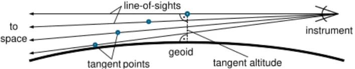
geoid
instrument
tangent points tangent altitude line-of-sights
to space
Fig. 1. A simple schematic of the measurement geometry of CRISTA-NF.
close to the subtropical jet is observed two-dimensionally at the resolution of vertically ≈0.5 km and horizontally
≈12.5 km (sampling along the flight-track) by an airborne infrared limb sounder. This paper improves upon work per-formed by Weigel et al. (2012), who evaluated a previous data version of the same flight with considerably less verti-cal resolution. As a result of an improved retrieval scheme, the cross sections exhibit a much improved vertical resolu-tion for the stratospheric trace gases ozone and nitric acid (see Appendix A), which in turn allows for the identification of previously non-resolvable fine-scale filaments in the ex-tratropical UTLS.
The trace gas cross sections show detailed filamentary structures, although the structures likely have a large extent orthogonal to the imaged plane. Backward-trajectories con-firm that these filaments are the result of stirring induced by breaking Rossby waves during the preceding days. In this paper, stirring refers to the large-scale folding and dynam-ical deformation of air masses (e.g. McIntyre and Palmer, 1984), while mixing refers to change of chemical composi-tion, within the scale of sampling, typically due to turbulent mixing. The state of mixing between UT and LS air in the filaments can be identified by the location of air parcels in tracer-tracer space. Mapping the tracer-tracer-space locations of air parcels to the geo-spatial space allows visualising the dynamical and chemical characteristics of the UTLS.
Two of the retrieved trace gas species are reactive nitrogen species. These can be used to derive a crude estimate of the total reactive nitrogen. The ratio between this estimate and the measured O3VMRs can serve as a simple indicator of
polluted air.
2 Measurements and model data
This paper is based largely on remote sensing measurements taken by CRISTA-NF during a test-flight for the African Monsoon Multidisciplinary Analysis (AMMA; see Cairo et al., 2010, and references therein) campaign and auxiliary global meteorological analyses data.
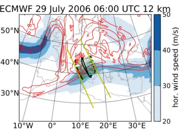
Fig. 2.Overview of aircraft flight path and meteorological situa-tion on 29 July 2006 06:00 UTC at 12 km altitude. Shown as blue surfaces are horizontal wind speeds. Shown as red contours are po-tential vorticity in PVU. The thick black line shows the flight path of M55-Geophysica. The horizontal position of every fourth tan-gent point of radiance measurements is shown as a small green cir-cle. Yellow dots highlight tangent points closest to 12 km altitude. The two yellow lines indicate the horizontal position of two vertical cross sections depicted in Fig. 3.
the line-of-sight is between ≈200 and 300 km, depending on the observed altitude. The optical system of CRISTA-NF consists of the centre telescope and two grating spec-trometers of the Space Shuttle experiment CRISTA that was successfully flown on the Shuttle Pallet Satellite (SPAS) in November 1994 (STS 66) and August 1997 (STS 85) (Of-fermann et al., 1999; Grossmann et al., 2002). CRISTA-NF employs 15 detectors for different wavelength regions, but for technical reasons only one operating in the wavenumber range from 776.0 to 868.0 cm−1is used here. A detailed dis-cussion of the instrument calibration is given by Schroeder et al. (2009). The instrument was deployed on board the high flying (up to 20 km for the discussed flight) Russian research aircraft M55-Geophysica viewing starboard.
Spatially highly resolved trace gas VMRs are determined from the spectrally resolved infrared radiance measurements. The given CRISTA-NF measurements allow for the deriva-tion of VMRs for the trace gas species of peroxyacetyl nitrate (PAN), nitric acid (HNO3), and ozone (O3). Water vapour
(H2O) and trichlorofluoromethane (CFC-11) were also
re-trieved with high quality, but the contrast in VMRs be-tween predominantly upper tropical tropospheric and pre-dominantly lowermost stratospheric air masses was much smaller than for the discussed species and thus less expres-sive. The retrieval process is summarised in Appendix A.
For analysis of the meteorological setting and also as in-put for the retrieval, operational analysis data supplied by the European Centre for Medium-range Weather Forecast (ECMWF) were used. For the given day of 29 July 2006, the analysis is available in six-hour time steps in the T799/L91
resolution, which corresponds to a horizontal resolution of
≈0.2◦×0.2◦with 91 levels between the surface and 80 km.
For the trajectory studies presented in Sect. 3.3, the tra-jectory model TRAJ3D (Bowman, 1993; Bowman and Car-rie, 2002) was used. The model is driven by winds from the Global Forecast System (GFS) final gridded analysis data sets (FNL) provided by the National Centers for Environ-mental Prediction (NCEP). These winds are available in six-hour time steps on a global grid of horizontally≈1.0◦×
1.0◦
with 26 pressure levels between 1000 and 10 hPa.
3 Analysis
3.1 A research flight following a breaking Rossby wave
The research flight discussed in this paper took place over Italy on 29 July 2006. The flight path of the M55-Geophysica is shown in Fig. 2. The ECMWF data presented in this figure show the meteorological setting on 29 July 2006, 06:00 UTC shortly before the actual flight. The aircraft took off in Verona at 06:54 UTC heading south-southeast towards the jet stream. The position of the jet stream can be roughly determined from horizontal wind speeds larger than≈20 m s−1at 12 km altitude in Fig. 2. The CRISTA-NF instrument was view-ing westwards durview-ing this portion of the flight. The tan-gent points illustrate roughly the geographic location of mea-sured air masses. At 07:30 UTC, the aircraft began a dive and performed a U-turn before heading back towards Verona at 08:00 UTC. During the following northbound leg of the flight, CRISTA-NF measured air masses east of the flight track. The flight path orthogonally crossed the 2 and 4 PVU contour lines that mark the approximate horizontal position of the transition region between the troposphere and the stratosphere at 12 km. This enabled CRISTA-NF to measure along comparably homogeneous air masses (as they are of similar potential vorticity), thereby reducing potential arte-facts induced by large gradients in temperature or trace gas VMRs along the line-of-sight of the instrument.
The distribution of wind speeds indicates a break of the jet stream during a wave breaking event. The position of the 2 PVU line follows roughly the position of the jet stream be-fore the wave breaking took place, which left a long-drawn filament of partly stratospheric air towards the west. The large area of potential vorticity between 2 and 4 PVU east of the flight track is a remnant of an earlier poleward wave breaking event, where a large portion of the jet stream was also cut off.
Fig. 3.Overview of meteorological situation on 29 July 2006 06:00 UTC. Depicted are two vertical cross sections, the horizontal positions of which are indicated as yellow lines in Fig. 2. Blue surfaces show horizontal wind speed. Red contours show potential vorticity in PVU. Yellow contours indicate potential temperature in Kelvin. Black dots indicate the position of primary and secondary lapse-rate tropopause. The dark grey rectangle indicates the approximate position of the measured trace gas cross sections presented later on.
are positioned horizontally to be most representative for the measurements taken at 12 km altitude. Further, there is also a varying time delay of up to three hours between the data points of the retrieved cross section and the model data pro-vided by ECMWF. The region of sampling is under double tropopause conditions during the flight period, as indicated in the figure. The primary and secondary tropopause levels shown in the figure are derived using the ECMWF tempera-ture profiles.
In both the western and the eastern cross section, the potential vorticity field identifies a tropopause fold, where stratospheric air intrudes along a baroclinic structure below the jet stream into the troposphere. The tropical tropopause (here at 16 to 17 km altitude) continues several hundred kilo-metres northward over this intrusion. Lower potential vortic-ity values just below this secondary tropopause further sug-gest a small tropospheric intrusion into the stratosphere just above the jet stream (see also Sect. 3.2). This is consistent with work of Pan et al. (2009) and Homeyer et al. (2011) as-sociating a double tropopause with such intrusions. Further, the observed region is known to be a place where the tropi-cal tropopause is often extended northwards during summer due to the influence of the monsoon circulation (e.g. Chen, 1995; Dunkerton, 1995). The potential vorticity in the low-ermost stratosphere below 16 km on the subtropical side of the jet stream also shows a very inhomogeneous structure. In the western cross section, a further intrusion of stratospheric air can be seen around 42◦
N, where the 6 PVU contour line extends well below the primary tropopause down to 10 km.
The potential temperature structure of the cross section shows typical characteristics of the subtropical transition. The 330–360 K isentropes show upward/downward inclina-tions above/below the jet core level, marked by the 355 K isentrope, as the flight moving equatorward across the jet. Although these are well known structures, we point it out to connect to the tracer structure shown later.
0.3
0.4
0.5 0.6 0.7 0.8
1.0 1.2
vert. resolution (km)
8
10
12
14
16
18
20
altitude (km)
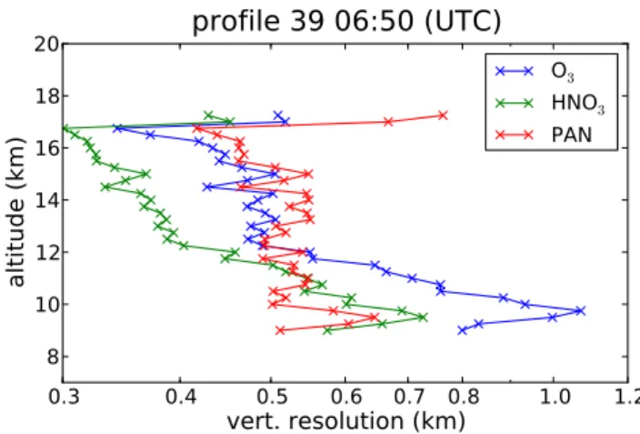
profile 39 06:50 (UTC)
O
3HNO
3PAN
Fig. 4.Vertical resolution for retrieved O3, HNO3, and PAN VMRs
for a representative profile of the western cross section.
There were few clouds seen during the flight above 8 km and all parcels, for which trace gas VMRs are derived, are cloud free.
3.2 Filamentary structure in observed trace gases
This section presents derived trace gas VMRs for O3, HNO3,
and PAN. Linearly derived precision and accuracy figures for the discussed species are given in Table 1; comparisons with measurements by other in situ and remote sensing instru-ments has ascertained the validity of these figures for a differ-ent research flight (see Ungermann et al., 2012). The vertical resolution is shown for an exemplary profile in Fig. 4. Note the excellent vertical resolution of HNO3, which is down to
0.3 km near the flight level. The vertical resolution deterio-rates towards lower altitudes due to a decreasing signal-to-noise ratio caused by lower VMRs for O3 and HNO3 and
a)
b)
c)
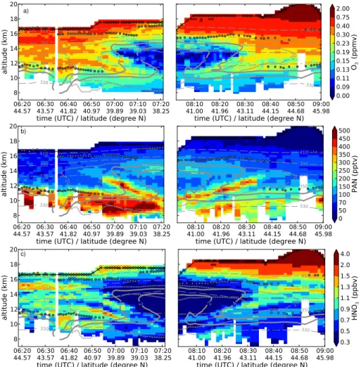
Fig. 5.Retrieved cross sections of O3(a), PAN(b), and HNO3(c). The left cross section shows the result of the westward pointing
measure-ments and the right cross section shows correspondingly the result of the eastward pointing measuremeasure-ments. Retrieved volume mixing ratios are depicted as coloured boxes. A discrete, non-linear colour scale was chosen to better highlight filamentary structures. The abscissa shows time of measurement and latitude at 12 km altitude. The altitude of M55-Geophysica at the time of measurement is indicated as a solid black line with crosses marking the time of successfully measured profiles. The position of primary and secondary lapse-rate tropopause are indi-cated by thick grey dots. The dotted grey lines show horizontal ECMWF wind speeds of 20 and 30 m s−1. The thick solid grey contour lines show ECMWF potential vorticity of 2 and 4 PVU. The thin dashed grey contour lines shows ECMWF isentropes. To generate the contours, the ECMWF model data were interpolated temporally and spatially to the horizontally closest tangent point. The white gap at 06:35 UTC marks a change in heading of the aircraft by 16◦where a profile was lost.
Table 1.Approximate precision and accuracy for discussed species as derived by linear diagnostics (Rodgers, 2000). The first number refers to values retrieved at instrument altitude, while the second number refers to values at altitudes≈8 km below the instrument.
species precision accuracy O3 40/20 ppbv 40/40 ppbv
PAN 10/20 pptv 20/20 pptv HNO3 0.2/0.1 ppbv 0.1/0.1 ppbv
Figure 5a shows two cross sections of O3 VMRs. Trace
gas VMRs above the flight level are not shown as they can-not be retrieved with a similar spatial resolution to those
be-low. The presence of clouds limits the retrieval at lower al-titudes. Retrieved temperature is used to derive primary and secondary thermal lapse-rate tropopause locations. ECMWF model data have been spatially (to the location of the closest tangent point) and temporally (to the time of measurement) interpolated onto the retrieved cross sections to provide fur-ther ancillary data. Accordingly, the positions of the 2 and 4 PVU potential vorticity surfaces, horizontal wind speeds of 20 and 30 m s−1, and selected isentropes are shown.
by gradients of temperature and trace gas VMRs along the line-of-sight, especially at altitudes below≈15 km.
The western cross section of O3 in Fig. 5a shows
sev-eral thin filamentary structures. Sevsev-eral tongues of strato-spheric air penetrate the subtropical jet stream. One long-drawn filament at 12 km altitude extends in a tropopause fold down to≈10 km; the vertical extent of this filament is
≈0.8 km. A second filament with increased O3VMRs is
lo-cated above, separated by a≈0.5 km thin layer of air with reduced O3 VMRs. This second O3 filament is located at
13.5 km altitude on the subtropical side of the jet stream and extends down to 12 km on the tropical side. A very small third tongue is located at 14 km altitude at 06:55 UTC and a fourth filament is positioned right below the tropopause be-tween 07:00 UTC and 07:10 UTC. On the subtropical side, a thin layer of reduced ozone VMR is visible just below the secondary tropopause suggesting an intrusion of tropo-spheric air that is consistent with reduced potential vortic-ity values in Fig. 3. The ozone VMRs below the subtrop-ical tropopause (here at 10 to 12 km altitude) are elevated to≈150 ppbv, presumably due to a combination of photo-chemical production in polluted air (see also HNO3and PAN
VMRs below) and mixing with stratospheric air. More typ-ical background O3values for this altitude range are on the
order of 50 to 100 ppbv (e.g. Murphy et al., 1993; Pan et al., 2007).
The eastern cross section provides a simpler picture, with overall reduced O3VMRs below 14 km. Still, two filaments
similar to the lower two filaments of the western cross section of elevated O3VMRs can be discerned that extend deep into
the tropopause fold: a rather weak filament located just above the subtropical tropopause and a more pronounced filament starting at 13.5 km and extending down to 11 km on the anti-cyclonic side.
Both PAN cross sections in Fig. 5b show high PAN VMRs below the subtropical tropopause greater than ≈400 pptv. Both cross sections show a filament with high PAN con-tent of above 300 pptv extending from about 13 km down to 10 km. The filament extends even up to 14 km, but with reduced VMRs of only 100 pptv. This filament nearly coin-cides with the upper edge of elevated O3VMRs inside the jet
stream; however, especially the lower portion seems to be lo-cated≈250 m lower. The highest VMRs occupy only one or two pixels vertically indicating a vertical extent of≈0.5 km. This filament seems to be not isentropic but covers instead a range of potential temperature from 365 K for the high-est altitude with a VMR of 300 pptv down to 335 K. Several factors may contribute to this discrepancy. First, both the in-trusion of PAN into the stratosphere as also the further de-velopment of the filamentary structure along the baroclinic jet stream may have been non-adiabatic. The tracer struc-ture may be capturing small-scale processes that are not rep-resented in the ECMWF analysis. An example for such a process are gravity waves from jet dynamics, as described in Zhang (2004). The pointing of the CRISTA-NF
instru-ment during the flight would not have allowed for the di-rect detection of such gravity waves, e.g. in retrieved tem-perature. Second, the ECMWF temperature model data may be mis-aligned in time and space with the actual physical structure; further artefacts might be introduced by the linear interpolation in time of the available model data. Last, the derived trace gas VMRs represent a complicated weighted mean along the line-of-sight of the instrument, being slightly different for each derived quantity, causing further misalign-ment with the ECMWF temperature data sampled at tangent point locations.
The measured PAN VMRs of 50 to 70 pptv in the low-ermost stratosphere are consistent with VMRs derived by Glatthor et al. (2007) from MIPAS measurements. Elevated PAN VMRs in the upper UTLS are probably caused by mix-ing with tropospheric air, which is supported by the close spatial proximity of air masses of PAN VMRs above 70 pptv to the tropical troposphere. According to Singh et al. (2007), a PAN VMR of 600 pptv below the subtropical tropopause is typical for polluted air masses.
The cross sections in Fig. 5c depict HNO3 VMRs. The
western cross section shows again the more layered struc-ture. Two HNO3filaments coincide with the lower two O3
filaments. The lowest filament even seems to extend down to 9.5 km around 07:20 UTC, but with VMRs so much de-creased that it cannot be readily distinguished from the pol-luted air found elsewhere in this altitude range. Both fila-ments continue horizontally northwards at least up to the profile measured at 06:35 UTC, where a change of the air-craft heading causes a gap in the cross section. The filament with reduced HNO3VMRs in between is likely
tropospheri-cally influenced, which is also supported by elevated CFC-11 VMRs (by 5 to 10 pptv compared to air masses above and be-low; not depicted).
At 06:38 UTC and 11 km altitude, an intrusion of strato-spheric air below the tropopause is suggested by increased HNO3VMRs and decreased PAN VMRs (see also Fig. 5b).
This intrusion is consistent with potential vorticity derived from ECMWF data.
The major features of the HNO3western cross section can
be found again in the eastern one, albeit mostly several hun-dred meters lower and with less steep gradients. The elevated HNO3VMRs around 8.5 km nearly coincide again with
ele-vated PAN VMRs, with HNO3VMR maxima being located
≈250 m above the PAN VMR maxima.
perpendicularly, implying that these air masses should not be trivially assigned to tropospheric or stratospheric origin ac-cording to their potential vorticity value. This suggests the work of non-conserving processes that modify both the en-tropy and the potential vorticity of the filaments. Except for the stratospheric intrusion around 06:38 UTC, the primary tropopause seems to clearly separate air masses. Close to the jet stream the temperature structure breaks down (be-tween 06:55 UTC and 07:15 UTC and be(be-tween 08:20 UTC and 08:40 UTC) and no thermal tropopause is detected at
≈11 km, even though the vertical gradients in all shown trace gases suggest a vertical boundary.
3.3 Wave breaking induced genesis of the observed filamentary structure
This section presents a backward trajectory analysis connect-ing the filamentary structure to the transport history of the air mass involved. Backward trajectories were calculated for the air masses sampled by the western cross section using NCEP-GFS wind fields. As HNO3VMRs show the most
ob-vious filamentary structure, positive HNO3 anomalies near
the jet stream are used to select air parcels with predom-inantly stratospheric origin. The corresponding trajectories show three dominant air streams. Further, a set of air parcels with high PAN VMRs close to the jet stream around 10 km altitude was added, as this is the region where the maxima of PAN VMRs do not perfectly coincide with the maxima of the HNO3 filament. Thus, these air parcels may show the best
connection to the tropospheric origin of PAN. The position of these four air streams, arriving in the western cross sec-tion on the final day, are shown as coloured circles in Fig. 6. To simplify the description, these sets of air parcels are re-ferred to by their relative mean vertical position surrounded by quotation marks and the employed colour in brackets in the following, e.g., as the “high-stratospheric (red)” filament. Four different air streams are identified:
– the “high-stratospheric (red)” filament, – the “middle-stratospheric (green)” filament, – the “low-stratospheric (blue)” filament, and the – the “tropospheric (black)” filament.
The “high-stratospheric (red)” and “high-stratospheric (green)” filament are selected to represent the filament with HNO3enhancement and lie mostly within the lower
strato-sphere poleward of the jet. The “low-stratospheric (blue)” fil-ament is selected to represent the HNO3enhanced air mass
below the tropopause and is associated with the stratospheric intrusion. Last, the “tropospheric (black)” filament is se-lected because this airmass of elevated PAN VMRs may give insight into the tropospheric sources of the PAN content of the more stratospheric filaments.
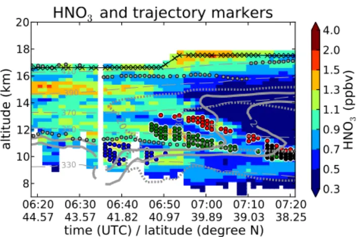
Fig. 6.Western cross section of HNO3 including markers of
se-lected air parcels. The red, green, blue and black circles mark the position of air parcels examined in the backward-trajectory simula-tions.
According to the backward trajectory simulations, the high HNO3 VMRs of greater than 0.9 ppbv in the upper
tropo-sphere of the western cross section are decidedly of tro-pospheric origin. These specific air parcels can be traced back to the Iberian peninsula. The trajectory studies suggest that the source region of the other polluted tropospheric air parcels is in North America.
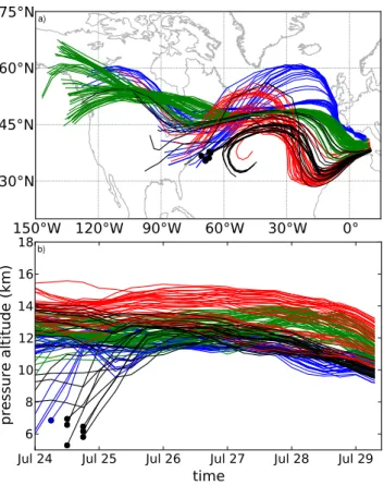
Figure 7 shows the horizontal and vertical movements of the selected sets of air parcels. The “tropospheric (black)” air stream contains several air parcels that were uplifted over the Atlantic Ocean close to the east coast of North Amer-ica, possibly by a warm conveyor belt (e.g. Stohl, 2001), to
≈12 km altitude and were then transported on the subtropical side of the jet stream towards Europe. While all tracked air parcels perform a downward movement during the two pre-ceding days, the vertical range (both in potential temperature and altitude) remains rather stable up to 25 July 2006.
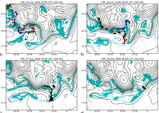
The genesis of the situation becomes more clear in Fig. 8 that shows the horizontal position of the air parcels marked in Fig. 6 in the same colours for four progressing time steps, each 36 h apart. The last figure corresponds to the position and situation shortly before the research flight. The meteoro-logical setting during the shown time frame is dominated by a cyclone in the North Atlantic on the one hand and a (weak-ening) anti-cyclone around 35◦N on the other hand. In
com-bination, they largely determine the flow of the air parcels and the jet stream.
a)
b)
Fig. 7.Backward-trajectories of four groups of selected air parcels.
(a)and(b)show the horizontal and vertical course of the trajecto-ries, respectively, for the five days preceding the measurement. The backward trajectory is terminated, if the parcel “sinks” below 7 km, whereby this last position is marked by a coloured dot. See also Fig. 6.
not mixing. However, the origin of the “tropospheric (black)” air parcels close to the lower half of the “high-stratospheric (red)” filament suggests strongly that the PAN found in the “high-stratospheric (red)” filament has the same source re-gion.
From Fig. 8, it is evident that all three sets of stratospheric air parcels have been part of the core of the subtropical jet at some point in time, but were differently advected by the breaking Rossby wave to finally arrive at the same desti-nation. As the signatures of tropospheric and stratospheric gases is much weaker for the eastern than for the western cross section, this suggests that these filaments do not ex-tend much further than the horizontal position of the eastern cross section. In combination with the distribution of poten-tial vorticity, the horizontal extent of the filaments along the jet stream should thus be smaller than≈15◦
of longitude or
≈1100 km.
Combining the results obtained from meteorological data with the CRISTA-NF measurements of vertical and horizon-tal extent across the jet stream, the filaments cover a vol-ume of roughly 1100×200×0.8 km3. All three predomi-nantly stratospheric filaments are entangled in between air
masses with significant tropospheric characteristics that were folded in during the breaking of the last baroclinic wave. The timescale involved in these stirring processes is rather short and numbers only a few days. By repeated folding, a very inhomogeneous structure with filaments of less than 0.8 km thickness is created.
3.4 Mixing and filaments in the extratropical transition layer
Trajectory analyses presented in the previous section indi-cate that the filamentary structure is created by large-scale dynamical processes including Rossby wave breaking. The trajectory calculations, however, are only representing advec-tion by the wind field. The formaadvec-tion of the observed struc-ture involves both advection and mixing (e.g. Konopka and Pan, 2012). In this case, small-scale processes such as tur-bulent mixing induced by the shear and strain in the flow, are also expected to contribute to the observed structure, which can be diagnosed using tracer-tracer relationships. Thus, this section explores the chemical characteristics of the observed trace gas structure using tracer-tracer relation-ships. This analysis aims to project the information gained in chemical tracer-tracer space to geo-spatial space. As a result, a highly resolved two-dimensional geo-spatial picture of the UTLS composition near the tropopause break reveals the ac-cumulative effect of advection and mixing of stratospheric and tropospheric air.
Our analyses focus on the tracer-tracer relationship be-tween O3and PAN, i.e., using O3as the stratospheric tracer
and PAN as the tropospheric tracer. O3is the most frequently
used stratospheric tracer. (e.g. Hoor et al., 2002; Pan et al., 2004). Using the flight data, 175 ppbv is used as a critical value to separate the stratospheric and tropospheric air mass. This threshold is higher than the typical 60 to 100 ppbv used in previous studies (compare Singh et al., 2007; Pan et al., 2007). This empirical threshold is based on the O3
distribu-tion in the sampling region from the retrieval. This higher value may be a combination of UT ozone retrieval uncer-tainty (see Table 1) and pollution in the sampled airmass.
As a tropospheric tracer, PAN has some different char-acteristics from the frequently used compounds such as CO and H2O. As a secondary pollutant, its sources are
biomass burning and anthropogenic pollution in the tropo-sphere (Stephens, 1969). Its lifetime is comparatively short, ranging from seconds in the lower troposphere to days and months in the uppermost troposphere (e.g. Roberts, 1990). 80 pptv of PAN were chosen as the threshold for stratospheric air, i.e., air parcels with less than 80 pptv are considered to be chemically stratospheric.
a) b)
d) c)
Fig. 8.Backward-trajectories of four groups of selected sets of air parcels. Black contour lines show geopotential height at 200 hPa. The cyan contour line indicates a potential vorticity of 1.5 PVU, while the cyan surface indicates a potential vorticity of 2 to 4 PVU at 200 hPa. The coloured circles correspond to the horizontal position of the similarly coloured air parcels highlighted in Fig. 6 at the time given in the respective title.
Fig. 9.The subsets of air parcels selected according to the four criteria and the slope derived for each set by the orthogonal distance regression (see Table 2). The western (left) and eastern (right) cross sections are shown separately. The precision of measurements is indicated by error bars in light grey.
variability between the stratospheric tracers and tropospheric tracers. In this case, a stratospheric branch is formed by the air mass with widely varying O3VMRs and low PAN VMRs,
and a tropospheric branch is formed by air mass with low O3
VMRs and high, widely varying PAN VMRs. We proceed to examine the O3-PAN relationship to identify mixing between
stratospheric and tropospheric air.
The relationship between PAN and O3for air parcels with
an O3 VMR below 175 ppbv (the chemically tropospheric
branch) or a PAN VMR below 80 pptv (the chemically strato-spheric branch) is depicted in Fig. 9 (subset of the data points) and Fig. 10 (all retrieved data points). The shape and clustering of the air parcels in tracer-tracer space suggest a further subdivision of air masses. In addition to the
men-tioned criteria (of low O3and PAN VMRs), the air masses
are further separated into the four categories listed in Ta-ble 2. The last column gives a descriptive name that fits the majority of the matching air parcels and which should be taken qualitatively (quotation marks highlight the use of these names in the following). The “clean tropospheric” air parcels stem from the Far East and are mostly located in the tropical troposphere above 12 km. In contrast, the “polluted tropospheric” air parcels were mostly advected from the west and most can be found in the upper subtropical troposphere. The chemically stratospheric air parcels are similarly split. A distinction is made according to the O3VMR, as a slope
a)
b)
Fig. 10.Relationship between PAN and O3. Both panels show the western (left) and eastern (right) cross sections separately.(a)shows
the location of air parcels in tracer-tracer space for all measured air parcels including error bars in light grey. Red colours indicate the stratospheric branch, purple colours indicate the tropospheric branch, and green colours indicate air parcels that could not be assigned to either category. Different shades of red are assigned according to O3VMR (with thresholds of 400 and 700 ppbv). Different shades of green
and purple are assigned according to PAN VMR (with thresholds of 150, 300, and 450 pptv).(b)shows the geo-spatial distribution of air parcels coloured according to their location in tracer-tracer space, i.e. with the same colours used in(a).
a)
b)
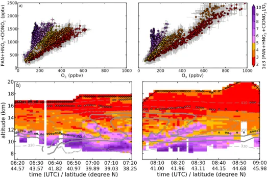
Fig. 11.Relationship of PAN+HNO3+ClONO2and O3. All panels show the western (left) and eastern (right) cross sections separately.
Table 2. Correlation between O3 and PAN for different air masses. The selection criteria are listed in the first two columns. The third
column gives the number ofnsamples matching the selection criteria. An orthogonal distance regression fits the formula of PAN(pptv)= a·O3(pptv)+b(pptv). Columns four and five giveaandbwith the number in brackets being the standard deviation for the last two digits. A descriptive name fitting to the majority of matching air parcels is given in the last column to simplify the description.
O3(ppbv) PAN (pptv) n a b(pptv) Descriptive name
<175 ≥150 600 1.114(79)×10−2 −1.27(11)×103 polluted tropospheric
<175 <150 447 9.33(65)×10−4 5.1(74)×100 clean tropospheric
<700 <80 914 −7.38(23)×10−5 9.51(11)×101 middleworld
≥700 <80 105 −2.34(28)×10−5 6.45(28)×101 overworld
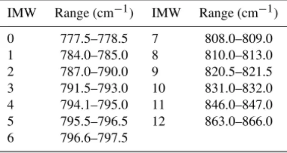
Table 3.A list of employed integrated microwindows (IMW) and their spectral range.
IMW Range (cm−1) IMW Range (cm−1) 0 777.5–778.5 7 808.0–809.0 1 784.0–785.0 8 810.0–813.0 2 787.0–790.0 9 820.5–821.5 3 791.5–793.0 10 831.0–832.0 4 794.1–795.0 11 846.0–847.0 5 795.5–796.5 12 863.0–866.0 6 796.6–797.5
lower flight level of the aircraft during the first part of the research flight did not allow for measurements at high alti-tudes. In the given meteorological setting, the position of the resulting two groups roughly coincides with air parcels in the middleworld (below≈420 K potential temperature; lower O3
VMRs) on the one hand and the overworld (above≈420 K potential temperature; higher O3VMRs) on the other hand.
For each set of air parcels, an orthogonal distance regres-sion (Boggs et al., 1987) was executed to derive PAN from O3 in a simple linear fashion taking the precision of both
trace gas measurements into account. The resulting coeffi-cients for all four sets are collected in Table 2. For each set of air parcels, the derived correlation is drawn as an appropri-ately coloured line in Fig. 9. The linear factor for “polluted tropospheric” air parcels is consistent with a similar regres-sion of boundary layer air performed by Wunderli and Gehrig (1991); however, the constant offset is larger in this case, in-dicating a larger background VMR of O3of 50 to 100 ppbv
that is consistent with typical O3 background values at this
altitude.
Figure 10a shows the location of all retrieved air parcels in tracer-tracer space. There is an obvious gap in the eastern scatter-plot between the “clean tropospheric” air parcels and the “middleworld” air parcels. Also, more mixed air parcels with high O3VMRs are found in the western cross section.
Assuming that mixing processes follow straight lines, this distribution of mixed air parcels implies that tropospheric air parcels with PAN VMR≥400 pptv were in close spa-tial proximity with stratospheric air parcels with an O3VMR
of at least 400 ppbv. This is consistent with previous stud-ies of STE that found frequent mixing between tropospheric and stratospheric air up to an O3 VMR of 400 ppbv (e.g.
Pan et al., 2004). In Fig. 5a, such air parcels can only be found upwards of≈14 km. This supports the hypothesis that the “high-stratospheric (red)” filament (referring to the red marked air parcels of Fig. 6) was generated by horizontal mixing between stratospheric and polluted tropospheric trop-ical air while circling the anti-cyclone at up to≈14 km. The upper half of this filament is thereby better mixed than the lower half, where the maxima of HNO3 and PAN are still
separable.
Figure 10b shows the geo-spatial position of categorised air parcels using the same colour scale that was used in Fig. 10a. Mixed air parcels (green shaded airmass) are clas-sified as ExTL (e.g. Pan et al., 2004, 2007). This is the first time that measurements allow the ExTL structure to be dis-played in a 2-D cross section. The three UTLS filaments of Sect. 3.3 can be readily identified, being categorised as con-sisting mostly of mixed air parcels.
The “high-stratospheric (red)” filament shows significant tropospheric influence up to 14 km altitude with especially high PAN VMRs around 12.5 km. In contrast, the upper por-tion of the “middle-stratospheric (green)” filament (referring to the green marked air parcels of Fig. 6) shows no tro-pospheric influence in its northern half above 12 km. How-ever, the lower half, being in close spatial proximity to the subtropical troposphere, shows significant signs of mixing. Also the “low-stratospheric (blue)” filament (referring to the blue marked air parcels of Fig. 6) mostly consists of air categorised as mixed. Figure 10b shows the filament of de-creased HNO3VMRs between the “high-stratospheric (red)”
and the “middle-stratospheric (green)” filament as consisting of mixed and stratospheric air. This filament consists likely of tropospheric air stemming from the clean upper tropical tro-posphere that contains only relatively low PAN VMRs. Thus, a rather small influx of stratospheric air with high O3VMRs
The vertical extent of the observed ExTL might be in-creased artificially due to the limited spatial resolution of the instrument. However, the vertical resolution at and above the thermal tropopause at 12 km is still≈0.5 km for all three trace gases, which limits the potential overestimation of the vertical depth to approximately the same amount.
The extratropical UTLS shows a layered and complex structure, consisting of different filaments that are at various stages of mixing. UTLS air parcels just around and above the primary tropopause and thereby closest to the troposphere are most obviously influenced by mixing with the tropo-spheric air. In general, the ExTL is formed approximately 1 km around the primary tropopause. It extends to about 2 km near the poleward (cyclonic) flank of the jet core. This struc-ture has been previously observed by in situ measurements that are limited to the flight track (Pan et al., 2007) and mod-elled (Konopka and Pan, 2012), but now it has been mapped out for the first time in a measured 2-D cross section. These new 2-D data reveal that the chemical air mass structure is very intricate and may often consist of multiple layers. The “high-stratospheric (red)” filament, consisting also of mixed air, extends up to 14 km altitude and more than 100 km north-wards into the UTLS. This suggests that the thermal and dy-namical tropopause exhibits breaks under the given meteoro-logical circumstances.
3.5 An NOyproxy for identifying pollution in the UTLS
This section introduces a proxy for the total reactive nitro-gen NOyfrom retrieved trace gases and uses this to estimate
the influence of tropospheric pollution on air masses in the UTLS. The NOyproxy proves especially useful when
com-bined with the available O3measurements. NOyand O3are
well correlated in the lower stratosphere. This is not a con-sequence of a direct chemical connection, but because their source regions, sink regions, and lifetimes are similar, so that their distribution is jointly determined mostly by transport and mixing processes (Murphy et al., 1993). As the correla-tion is especially strong in the lowermost stratosphere, devi-ations thereof may be used to determine the origin of mea-sured air masses.
The total reactive nitrogen plays an important role in the polluted and unpolluted atmosphere. It mainly consists of NO, NO2, PAN, HNO3, HO2NO2, and alkyl and
multifunc-tional nitrates. According to Singh et al. (2007), PAN, HNO3,
and NOx(=NO+NO2) are the major contributors to NOyin
the extratropical UTLS with a combined fractional percent-age of about 95 % on averpercent-age. NO2 reacts with OH and a
third-body to HNO3, which is in turn converted back to NO2
(and OH) by photolysis. In the altitude range of the UTLS, the conversion to HNO3is much faster than its destruction,
so any stable equilibrium between NO2and HNO3will
heav-ily favour HNO3(Austin et al., 1986). As there are no NOx
estimates available from CRISTA-NF measurements, only a proxy for NOycan be formed by the sum of the available
dominant contributors PAN, HNO3, and ClONO2. The latter
trace gas could be neglected for the current atmospheric sit-uation but would be important for the analysis of polar mea-surements. In the measurements of Singh et al. (2007), NOx
was the major constituent of NOy close to the troposphere,
so the given NOyproxy might underestimate the true NOyby
a factor of 2 to 3, depending on the altitude. But in contrast to the measurements of Singh et al. (2007), most of the air mea-sured by CRISTA-NF should be free of recent influx caused by convection, so the NOxcontent should be much lower and
the HNO3content much higher due to prolonged ageing.
Us-ing the satellite instrument UARS, Morris et al. (1997) found a ratio of just 0.1 between NOxand NOyat 550 K (≈22 km),
implying that the proxy should become more reliable towards the flight level.
The ratio between NOyand O3is remarkably constant in
the lower stratosphere and removes a lot of the inherent vari-ability of the individual species. According to the measure-ments of Murphy et al. (1993), typical values for the ratio above 430 K potential temperature in the region observed by CRISTA-NF are 0.003 to 0.004. Even though the available proxy likely underestimates NOy, one can still deduce that
a ratio larger than 0.004 indicates tropospheric influx of NOy.
The relationship between the NOy proxy
(PAN+HNO3+ClONO2) and O3is depicted in Fig. 11a.
The air parcels with the lowest VMRs of either the NOy
proxy or O3 are again those of the upper tropical
tropo-sphere. Further, there is a set of predominantly stratospheric air parcels following the ratio of 0.002 to 0.004. Air parcels with a ratio above 0.006 certainly consist of polluted air. The air parcels with ratios in between consist of less polluted or mixed air. The geo-spatial distribution of the air parcels is shown in Fig. 11b. The state of air parcels with a ratio below 0.004 cannot be determined reliably due to the missing NOx. However, assuming that the measured air masses were
not subject to a recent influx of freshly polluted air, air parcels with a ratio below 0.003 should consist of unpolluted stratospheric air (at the typical altitudes and location where these air parcels are found, HNO3 should be the major
contributor so that the correct ratio of NOy/O3 should still
be less than 0.004 regardless of the NOxcontent).
In situ measurements for NOx, NOy, and O3 are usually
available for such research flights. But this specific flight was a test flight, where not all instrumentation was mounted or turned on. For other campaigns, one might improve the proxy by identifying the correlations between NOx and available
species and thereby derive an estimate for NOxby multiple
linear regression. Still, if not all types of sounded air masses are also sampled by the in situ instruments, artefacts may arise due to the different history and ageing of air (Singh et al., 2007). In either case, this approach should reduce the error of the NOyestimate significantly.
significant tropospheric influence, as indicated by slightly elevated PAN and decreased HNO3 VMRs below the
sec-ondary tropopause in the western cross section, is therefore likely from the upper tropical troposphere. The increased ra-tios in the upper tropical troposphere between 12 and 14 km altitude are most likely an artefact caused by noise in the re-trieved O3VMRs, which affects the ratio more strongly for
the very low O3VMRs found in this region.
The previously discussed “high-stratospheric (red)” fila-ment (see Fig. 6) is clearly marked by an increased ratio as high as 0.009 decreasing to ≈0.004 in its uppermost part. Here, the influence and reach of polluted tropospheric air on UTLS is most visible. The corresponding filament in the western cross section shows this even better. Also the “low-stratospheric (blue)” air parcels of the “low-stratospheric intrusion contain obviously elevated NOylevels.
The ratio between the NOyproxy and O3shows the
pol-lution of involved air masses more clearly than the individ-ual trace gases. Especially HNO3exhibits a very filamentary
structure in the UTLS, which is simplified by constructing the ratio. Thus, this technique enables a simple view on the pollution of air masses derivable fully from CRISTA-NF in-frared remote sensing measurements.
4 Discussion and conclusions
This study presented a set of highly resolved trace gas cross sections derived from limb sounder measurements of CRISTA-NF. These trace gas cross sections, bridging the measurement gap between airborne in situ measurements and satellite-borne remote sensing instruments, represent the first multi-species 2-D chemical structure of the subtropical UTLS following an event of Rossby wave breaking. The pre-sented data and analyses bring forth a number of new insights into chemical transport and chemical structure between the stratosphere and troposphere.
The observations showed a heavily layered structure with alternating filaments of predominantly stratospheric and tro-pospherically influenced air. The extent of the observed fil-aments is ≈0.8 km vertically and ≈200 km in across-jet-stream direction. Fine-scale filamentary structure near the tropopause has been predicted by an idealised model (con-tour advection) as a consequence a dynamical stretching by the large-scale flow (Appenzeller et al., 1996). These fila-mentary structures, however, are often analysed on isentropic surfaces. The presented results show that these structures also exist in the vertical and that they may not always be aligned with the isentropes.
Backward trajectory analyses revealed that stirring by the jet dynamics resulted in the observed layered structure. Strong gradients in trace gas VMRs were observed along isentropes, especially in the vicinity of the tropopause fold. This may indicate that the processes leading up to the im-aged situation involve non-adiabatic processes such as
up-lift by a warm conveyor belt or gravity waves instigated by the baroclinic jet stream. Partly, this may be an artefact of an imperfect alignment between ECMWF temperature data and the position of retrieved trace gas parcels. As the tra-jectory calculations take into account only purely advective processes, it is important to complement this analysis with tracer-tracer relationships to identify mixing processes.
Having available multiple trace gas species offered the opportunity to characterise the chemical composition struc-ture of the observed region in tracer-tracer space. The VMRs of O3and PAN were used to identify predominantly
tropo-spheric and stratotropo-spheric air masses. Connecting these re-sults from tracer-tracer space with the geo-spatial space al-lowed for the first time deriving highly resolved cross sec-tions with clear identification of a highly structured ExTL close to the subtropical jet stream. Due to a lack of high reso-lution measurements, the ExTL is often perceived as a homo-geneous mixing layer around the tropopause (e.g. Gettelman et al., 2011). The presented results show that the real atmo-sphere is likely much more complicated, and that the ExTL is likely highly structured and inhomogeneous.
In addition, the influence of polluted tropospheric air masses on the stratosphere was examined using the sum of HNO3, ClONO2, and PAN divided by O3. This ratio is rather
stable in the lower stratosphere and deviations indicate ab-normal chemical processes (such as occur in the polar win-ter) or mixing with (polluted) tropospheric air masses. This ratio complemented the picture given by the O3-PAN
rela-tionship and showed the influence of pollution to be largely restricted to the ExTL.
In combination, this demonstrates a rich spatial struc-ture of the UTLS region at the subtropical jet, where the tropopause break is perturbed by breaking Rossby waves. The induced stirring brings into close contact air masses from stratospheric and tropospheric origin resulting in a complex structure of entangled filaments. How long does it take the observed filaments to lose their characteristics due to diffu-sion, small-scale turbulence, and further stirring? In the given meteorological setting (end of July over the Northern At-lantic), wave breaking could be observed on nearly a daily basis. These filamentary structures are likely a ubiquitous feature of the subtropical UTLS. We may ask, what is the effect of this layered structure on chemical and radiative pro-cesses? How should they be represented in global chemistry-climate models? Most global chemistry-chemistry-climate models rep-resent the UTLS with a vertical resolution of≈1 km or worse (e.g. Hegglin et al., 2010), which is not sufficient to repro-duce the observed fine-scale structure. These questions de-mand more high-resolution measurements of this kind, be-yond the spatial and temporal coverage provided by this sin-gle flight.
excellent resolution proved sufficient but also needed to map the very fine details and structures in the UTLS. An instru-ment with a smaller field-of-view and finer sampling might even achieve a better vertical resolution and reproduce more details.
The evaluation of measurements was hindered in this case by the limited spectral range and spectral resolution available for the given flight. A modern airborne limb imager would have been able to retrieve more species at even higher verti-cal and horizontal resolution (Ungermann et al., 2011). Us-ing near-future satellite infrared limb imagers, several par-allel cross sections of only slightly reduced quality will be attainable from space (ESA, 2012). Such a satellite-borne instrument would have the obvious advantage of providing three-dimensional global coverage for several years to come, allowing for the deduction of, e.g. a filament climatology and the direct observation of the development of such filaments in time, which would allow quantitative insight in the stirring and mixing processes. Thus, infrared limb imagers prove as a valuable tool for the study of the highly complex UTLS region.
Appendix A
Retrieval
This appendix shortly recaptures the retrieval of trace gas VMRs from spectrally resolved infrared radiances measured by the CRISTA-NF instrument. A detailed description of the first retrieval of this set of measurements is given by Weigel et al. (2012). Ungermann et al. (2012) improved this setup by employing a more accurate line-of-sight determination and a finer retrieval grid. In addition, horizontal regularisation was added to lower the impact of stochastic error sources on the results (see Ungermann, 2013).
Retrieving trace gas VMRs from limb sounder measure-ments is an ill-posed problem. This implies that many or no trace gas profiles might fit to the imperfect measurements and that small measurement errors may have a large effect on retrieved VMRs. One counter-acts this by approximat-ing the original ill-posed problem by a (well-posed) prob-lem that is less affected by these probprob-lems. This approxima-tion is often called regularisaapproxima-tion (e.g. Tikhonov and Ars-enin, 1977; Rodgers, 2000). Here, the approximation of min-imising a quadratic form, i.e. the cost functionJ:Rn7→R is used to identify a unique solution:
J (x)=(F (x)−y)TS−1ǫ (F (x)−y)+(x−xa)TS−1a (x−xa). (A1)
The vectorxrepresents the atmospheric state of a cross
sec-tion (assuming homogeneity in the line-of-sight direcsec-tion) and some instrument parameters. The vector y consists of
the measured radiances. The functionF :Rn7→Rmis a (for-ward) model that produces synthetic measurements given an atmospheric state. The matrixSǫ is a covariance matrix
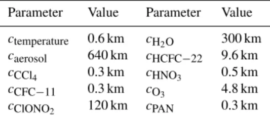
de-Table A1.Correlation lengths employed for the regularisation.
Parameter Value Parameter Value
ctemperature 0.6 km cH2O 300 km caerosol 640 km cHCFC−22 9.6 km
cCCl4 0.3 km cHNO3 0.5 km
cCFC−11 0.3 km cO3 4.8 km cClONO2 120 km cPAN 0.3 km
scribing the available knowledge about measurement errors. The vectorxa and associated covariance matrixSa describe
the available a priori knowledge about the atmospheric state. A set of 12 integrated microwindows is employed in this multi-target retrieval. A comprehensive list is given in Ta-ble 3. The quantities of temperature, aerosol (extinction), CCl4, CFC-11, ClONO2, HCFC-22, H2O, HNO3, O3, and
PAN are retrieved. The primary targets are HNO3, O3, and
PAN, while the remainder is mostly retrieved to reduce systematic errors in the primary targets. ECMWF analysis data is used as a priori for temperature, pressure, and water vapour. For PAN, a zero profile is employed. The other tar-gets are initialised using the climatology of Remedios et al. (2007).
The gases C2H6, HCFC-22, HNO4, 12, and
CFC-114 contribute a small percentage to the measured radiation and thus have to be included in the forward model. Further, the VMRs of CO2have to be adjusted for the annual increase
and inter-annual variability. The discussed results are not sensitive to the assumed VMRs for these gases. However, the simulated radiances agree better with the measured radiances when these gases are initialised according to a model run of the Whole Atmosphere Community Climate Model, version 4 (WACCM4; Garcia et al., 2007). The specific parametrisa-tion for the used model run can be found in the publicaparametrisa-tions of Lamarque et al. (2012) and Kunz et al. (2011b). While it is plausible that the use of WACCM model data reduces the systematic error caused by these background gases, their as-sumed standard deviations were not correspondingly reduced for the estimation of retrieval accuracy.
The a priori covariance matrix is assembled by Tikhonov regularisation modelled after the auto-regressive model of optimal estimation (see Ungermann et al., 2012). In effect, a constraint on the deviation of absolute value from the a pri-ori vectorxais combined with two constraints on the
devia-tion between the derivatives of the state vectorx in vertical
vertical and horizontal scales of synoptic structures. These parameters were chosen as result of a parameter study with the intent of using the weakest possible constraints for the primary targets while keeping visible noise to a minimum. Care was taken so that no isentropic structures were intro-duced by the application of isentropic regularisation that are not also discernible in the underlying radiances and conven-tional 1-D retrievals.
The weight of the a priori absolute value constraint is re-duced by a factor of 10 compared to the constraints on the derivative. This reduces the bias of the absolute values of the solution towards the a priori vector and increases the mea-surement contribution.
The true measurement error covariance matrix is approx-imated by an uncorrelated error budget of 1 %. The major components of the measurement error are uncertainty in el-evation angle of the measurement and noise of the detector. The chosen budget very likely overestimates the combined error and might thereby be partly responsible for the small correlation lengths in Table A1. This would imply that the supplied precision figures overestimate the true precision.
The model and retrieval software employed for the sim-ulation of radiances is the Jülich Rapid Spectral Simsim-ulation Code Version 2. This Python/C++–based model and its pre-decessor were used in several experiments and studies (e.g. Hoffmann et al., 2008; Eckermann et al., 2009; Ungermann et al., 2010). The joint retrieval of the western cross section poses a problem with 32 224 unknowns and 26 584 measured radiances (the eastern one is similar). All involved matri-ces are stored using sparse representations. The minimisation of the cost-function is performed using a truncated quasi-Newton method employing conjugate gradients for the so-lution to the posed linear equation systems. It requires five iterations for the given setup and thereby five evaluations of the Jacobian matrix that are calculated by an analytic ad-joint model (Lotz et al., 2012). Using eight cores, this is ac-complished in 18 min. Providing the diagnostic parameters of precision, accuracy, and measurement contribution takes another 17 min on the same eight cores.
Acknowledgements. D. E. Kinnision, NCAR, is thanked for kindly providing the WACCM4 model data used in the retrieval. K. Bow-man is thanked for making his trajectory model TRAJ3D available for this study. We sincerely thank A. Dudhia, Uni. Oxf., for pro-viding the Reference Forward Model (RFM) used to calculate the optical path tables required by our forward model. The team of the Michelson Interferometer for Passive Atmospheric Sounding – Aircraft (MIPAS-STR) is thanked for providing their attitude mea-surements that significantly improved our retrievals. We especially thank M. Shapiro, B. Ridley, F. Flocke, and many other National Center for Atmospheric Research (NCAR) scientists for fruitful dis-cussions.
The AMMA-SCOUT-O3 measurement campaign was facili-tated by the European Commission and the EC Integrated Project SCOUT-O3 (505390-GOCE-CT-2004) and AMMA. Based on a
French initiative, AMMA was set up by an international scientific group and is currently funded by a large number of agencies. It has been the beneficiary of a major financial contribution from the Eu-ropean Communities Sixth Framework Research Program.
J. Ungermann was supported by the Deutsche Forschungsge-meinschaft (GZ UN 311/1-1 and GZ KA2324/1-2) and the visitor’s program of the Atmospheric Chemistry Division at the NCAR. NCAR is funded by the National Science Foundation (NSF). The European Centre for Medium-Range Weather Forecasts (ECMWF) and the National Centers for Environmental Prediction (NCEP) are acknowledged for meteorological data support. The NCEP-GFS data for this study are from the Research Data Archive (RDA) which is maintained by the Computational and Information Sys-tems Laboratory (CISL) at NCAR. The original data are available from the RDA (http://rda.ucar.edu) in data set number ds083.2.
The service charges for this open access publication have been covered by a Research Centre of the Helmholtz Association.
Edited by: T. J. Dunkerton
References
Appenzeller, C., Davies, H. C., and Norton, W. A.: Fragmentation of stratospheric intrusions, J. Geophys. Res., 101, 1435–1456, doi:10.1029/95JD02674, 1996.
Austin, J., Garcia, R. R., Russell III, J. M., Solomon, S., and Tuck, A. F.: On the Atmospheric Chemistry of Nitric Acid, J. Geophys. Res., 91, 5477–5485, doi:10.1029/JD091iD05p05477, 1986. Bernath, P. F., McElroy, C. T., Abrams, M. C., Boone, C. D.,
But-ler, M., Camy-Peyret, C., Carleer, M., Clerbaux, C., Coheur, P.-F., Colin, R., DeCola, P., DeMazière, M., Drummond, J. R., Du-four, D., Evans, W. F. J., Fast, H., Fussen, D., Gilbert, K., Jen-nings, D. E., Llewellyn, E. J., Lowe, R. P., Mahieu, E., Mc-Connell, J. C., McHugh, M., McLeod, S. D., Michaud, R., Mid-winter, C., Nassar, R., Nichitiu, F., Nowlan, C., Rinsland, C. P., Rochon, Y. J., Rowlands, N., Semeniuk, K., Simon, P., Skel-ton, R., Sloan, J. J., Soucy, M.-A., Strong, K., Tremblay, P., Turn-bull, D., Walker, K. A., Walkty, I., Wardle, D. A., Wehrle, V., Zander, R., and Zou, J.: Atmospheric Chemistry Experiment (ACE): mission overview, Geophys. Res. Lett., 32, L15S01, doi:10.1029/2005GL022386, 2005.
Berthet, G., Esler, J. G., and Haynes, P. H.: A Lagrangian perspective of the tropopause and the ventilation of the lowermost stratosphere, J. Geophys. Res., 112, D18102, doi:10.1029/2006JD008295, 2007.
Boggs, P. T., Byrd, R. H., and Schnabel, R. B.: A stable and efficient algorithm for nonlinear orthogonal distance regression, SIAM J. Sci. Stat. Comput., 8, 1052–1078, doi:10.1137/0908085, 1987. Bowman, K. P.: Large-scale isentropic mixing properties of the
Antarctic polar vortex from analyzed winds, J. Geophys. Res., 98, 23013–23027, doi:10.1029/93JD02599, 1993.
Bowman, K. P. and Carrie, G. D.: The mean-meridional transport circulation of the troposphere in an idealized GCM, J. Atmos. Sci., 59, 1502–1514, doi:10.1175/1520-0469(2002)059<1502:TMMTCO>2.0.CO;2, 2002.
Berthe-lier, J. J., Blom, C., Christensen, T., D’Amato, F., Di Don-francesco, G., Deshler, T., Diedhiou, A., Durry, G., Engelsen, O., Goutail, F., Harris, N. R. P., Kerstel, E. R. T., Khaykin, S., Konopka, P., Kylling, A., Larsen, N., Lebel, T., Liu, X., MacKenzie, A. R., Nielsen, J., Oulanowski, A., Parker, D. J., Pelon, J., Polcher, J., Pyle, J. A., Ravegnani, F., Rivière, E. D., Robinson, A. D., Röckmann, T., Schiller, C., Simões, F., Ste-fanutti, L., Stroh, F., Some, L., Siegmund, P., Sitnikov, N., Vernier, J. P., Volk, C. M., Voigt, C., von Hobe, M., Viciani, S., and Yushkov, V.: An introduction to the SCOUT-AMMA strato-spheric aircraft, balloons and sondes campaign in West Africa, August 2006: rationale and roadmap, Atmos. Chem. Phys., 10, 2237–2256, doi:10.5194/acp-10-2237-2010, 2010.
Chen, P.: Isentropic cross-tropopause mass exchange in the extratropics, J. Geophys. Res., 100, 16661–16673, doi:10.1029/95JD01264, 1995.
Danielsen, E. F.: Stratospheric-tropospheric exchange based on radioactivity, ozone, and potential vortic-ity, J. Atmos. Sci., 25, 502–518, doi:10.1175/1520-0469(1968)025<0502:STEBOR>2.0.CO;2, 1968.
Dunkerton, T.: Evidence of meridional motion in the summer lower stratosphere adjacent to monsoon regions, J. Geophys. Res., 100, 16675–16688, doi:10.1029/95JD01263, 1995.
Eckermann, S. D., Hoffmann, L., Höpfner, M., Wu, D. L., and Alexander, M. J.: Antarctic NAT PSC belt of June 2003: observa-tional validation of the mountain wave seeding hypothesis, Geo-phys. Res. Lett., 36, L02807, doi:10.1029/2008GL036629, 2009. ESA: Report for Mission Selection: PREMIER, vol. SP-1324/3, ESA Communication Production Office, Noordwijk, The Nether-lands, 2012.
Fischer, H., Birk, M., Blom, C., Carli, B., Carlotti, M., von Clar-mann, T., Delbouille, L., Dudhia, A., Ehhalt, D., EndeClar-mann, M., Flaud, J. M., Gessner, R., Kleinert, A., Koopman, R., Langen, J., López-Puertas, M., Mosner, P., Nett, H., Oelhaf, H., Perron, G., Remedios, J., Ridolfi, M., Stiller, G., and Zander, R.: MIPAS: an instrument for atmospheric and climate research, Atmos. Chem. Phys., 8, 2151–2188, doi:10.5194/acp-8-2151-2008, 2008. Friedl-Vallon, F., Riese, M., Maucher, G., Lengel, A., Hase, F.,
Preusse, P., and Spang, R.: Instrument concept and preliminary performance analysis of GLORIA, Adv. Space Res., 37, 2287– 2291, doi:10.1016/j.asr.2005.07.075, 2006.
Garcia, R. R., Marsh, D., Kinnison, D. E., Boville, B., and Sassi, F.: Simulations of secular trends in the mid-dle atmosphere 1950–2003, J. Geophys. Res., 112, D09301, doi:10.1029/2006JD007485, 2007.
Gettelman, A., Hoor, P., Pan, L. L., Randel, W. J., Heg-glin, M. I., and Birner, T.: The extra tropical upper tropo-sphere and lower stratotropo-sphere, Rev. Geophys., 49, RG3003, doi:10.1029/2011RG000355, 2011.
Gille, J. C., Barnett, J., Arter, P., Barker, M., Bernath, P., Boone, C., Cavanaugh, C., Chow, J., Coffey, M., Craft, J., Craig, C., Di-als, M., Dean, V., Eden, T., Edwards, D. P., Francis, G., Halvor-son, C., Harvey, L., Hepplewhite, C., Khosravi, R., KinniHalvor-son, D., Krinsky, C., Lambert, A., Lee, H., Lyjak, L., Loh, J., Mankin, W., Massie, S., McInerney, J., Moorhouse, J., Nardi, B., Pack-man, D., Randall, C., Reburn, J., Rudolf, W., Schwartz, M., Serafin, J., Stone, K., Torpy, B., Walker, K., Waterfall, A., Watkins, R., Whitney, J., Woodard, D., and Young, G.: The High-Resolution Dynamics Limb Sounder: Experiment overview,
re-covery, and validation of initial temperature data, J. Geophys. Res., 113, D16S43, doi:10.1029/2007JD008824, 2008. Glatthor, N., von Clarmann, T., Fischer, H., Funke, B.,
Grabowski, U., Höpfner, M., Kellmann, S., Kiefer, M., Lin-den, A., Milz, M., Steck, T., and Stiller, G. P.: Global peroxy-acetyl nitrate (PAN) retrieval in the upper troposphere from limb emission spectra of the Michelson Interferometer for Passive At-mospheric Sounding (MIPAS), Atmos. Chem. Phys., 7, 2775– 2787, doi:10.5194/acp-7-2775-2007, 2007.
Grossmann, K. U., Offermann, D., Gusev, O., Oberheide, J., Riese, M., and Spang, R.: The CRISTA-2 mission, J. Geophys. Res., 107, 8173, doi:10.1029/2001JD000667, 2002.
Haynes, P., Scinocca, J., and Greenslade, M.: Forma-tion and maintenance of the extratropical tropopause by baroclinic eddies, Geophys. Res. Lett., 28, 4179–4182, doi:10.1029/2001GL013485, 2001.
Hegglin, M. I., Boone, C. D., Manney, G. L., and Walker, K. A.: A global view of the extratropical tropopause transition layer from Atmospheric Chemistry Experiment Fourier Transform Spectrometer O3, H2O, and CO, J. Geophys. Res., 114, D00B11,
doi:10.1029/2008JD009984, 2009.
Hegglin, M. I., Gettelman, A., Hoor, P., Krichevsky, R., Manney, G., Pan, L. L., Son, S.-W., Stiller, G., Tilmes, S., Walker, K. A., Eyring, V., Shepherd, T. G., Waugh, D., Akiyoshi, H., Anel, J. A., Austin, J., Baumgaertner, A., Bekki, S., Braesicke, P., Brühl, C., Butchart, N., Chipperfield, M., Dhomse, S., Frith, S., Garny, H., Hardiman, S., Jöckel, P., Kinnison, D., Lamar-que, J., Mancini, E., Michou, M., Morgenstern, O., Naka-mura, T., Olivié, D., Pawson, S., Pitari, G., Plummer, D., Pyle, J., Rozanov, E., Scinocca, J., Shibata, K., Smate, D., Teyssèdre, H., Tian, W., and Yamashita, Y.: Multimodel assessment of the up-per troposphere and lower stratosphere: extratropics, J. Geophys. Res., 115, D00M09, doi:10.1029/2010JD013884, 2010. Hintsa, E. J., Boering, K. A., Weinstock, E. M., Anderson, J. G.,
Gary, B. L., Pfister, L., Daube, B. C., Wofsy, S. C., Loewen-stein, M., Podolske, J. R., Margitan, J. J., and Bui, T. P.: Troposphere-to-stratosphere transport in the lowermost strato-sphere from measurements of H2O, CO2, N2O and O3, Geophys.
Res. Lett., 25, 2655–2658, doi:10.1029/98GL01797, 1998. Hoerling, M. P., Schaack, T. K., and Lenzen, A. J.: Global objective
tropopause analysis, Mon. Weather Rev., 119, 1816–1831, 1991. Hoffmann, L., Kaufmann, M., Spang, R., Müller, R., Reme-dios, J. J., Moore, D. P., Volk, C. M., von Clarmann, T., and Riese, M.: Envisat MIPAS measurements of CFC-11: retrieval, validation, and climatology, Atmos. Chem. Phys., 8, 3671–3688, doi:10.5194/acp-8-3671-2008, 2008.
Holton, J. R., Haynes, P. H., McIntyre, M. E., Douglass, A. R., Rood, R. B., and Pfister, L.: Stratosphere–troposphere exchange, Rev. Geophys., 33, 403–439, 1995.
Homeyer, C. R., Bowman, K. P., Pan, L. L., Atlas, E. L., Gao, R.-S., and Campos, T. L.: Dynamical and chemical characteristics of tropospheric intrusions observed during START08, J. Geophys. Res., 116, D06111, doi:10.1029/2010JD01509, 2011.
Hoor, P., Fischer, H., Lange, L., Lelieveld, J., and Brunner, D.: Sea-sonal variations of a mixing layer in the lowermost stratosphere as identified by the CO-O3 correlation from in situ