Application of He's homotopy perturbation method for solving nonlinear wave-like equations with variable coefficients

Volume , )ssue : pp. - 9

Available online at www.ijaamm.com ISSN: 2347-2529

Application of He's homotopy perturbation method for

solving nonlinear wave-like equations with variable

coefficients

Sumit Gupta a, Devendra Kumar a,1 and Jagdev Singh b

a,

Department of Mathematics, Jagan Nath Gupta Institute of Engineering and Technology, Jaipur-302022, Rajasthan, India

b

Department of Mathematics, Jagan Nath University, Jaipur-303901, Rajasthan, India

Received 07 October 2013; Accepted (in revised version) 13 November 2013

A B S T R A C T

In this paper, we apply homotopy perturbation method (HPM) for solving nonlinear wave-like equations with variable coefficients. HPM yields solution in rapid convergent series from easily computable terms, and in some cases, yields exact solutions in one iteration. Moreover, this technique does not require any discretization, linearization or small perturbations and therefore reduces the numerical computations to a great extent. The solution procedure by HPM is simple yet highly accurate and compares favorably with the exact solutions obtained early in the literature. The methodology presented in the paper is useful for highly nonlinear problems consisting of more than one differential equation.

Keywords: Homotopy perturbation method, Nonlinear wave-like equations, Approximate solutions, Exact solutions, Mathematica.

MSC 2010 codes:39B12, 35F25, 35C10

© 2013 IJAAMM

1 Introduction

The homotopy perturbation method introduced by the Chinese researcher Dr. Ji Huan He in 1998, has come to be accepted as an elegant tool in the hands of researchers looking for simply yet highly effective solutions to complicated problems in many diverse areas of science and technology. In a series of papers He (1999, 2003) has outlined and refined the HPM, showing its usefulness by nonlinear differential equations. As a rule, HPM tends to produce much more elegant solutions as compared to the other competing techniques such as homotopy analysis method (HAM), regular perturbation methods etc., yet it is not at the cost of accuracy. In general the solutions produced by the HPM are as accurate as the solutions

given by the other approximate methods. Recently, He has provided a highly reliable account of the HPM in a monograph (He 2000a).

The HPM is in fact, a coupling of the traditional perturbation method and homotopy in topology (He 2000b). The method yields a very rapid convergence of the solution series in most cases, usually only few iterations produce very accurate solutions. This method was applied to functional integral equations (Abbasbandy 2007), coupled system of reaction-diffusion equation (Ganji and Sadighi 2006), to Helmholtz equation and fifth-order KdV equation (Rafei and Ganji 2006), the epidemic model (Rafei et al. 2007), determining the frequency-amplitude relation of a nonlinear oscillator with discontinuity (Ozis and Yildirim 2007a), travelling wave solution of the KdV equation (Ozis and Yildirim 2007b). Momani and Odibat (2007) and Odibat and Momani (2008) suggested a modified HPM and used it for nonlinear partial differential equations of fractional order and quadratic Riccati differential equation of fractional order. It was applied to the thin film flow of a fourth grade fluid down an inclined plane (Siddique et al. 2006), to the nonlinear Voltera-Fredholm integral equation (Ghasemi et al. 2007), to the singular VIE of second order (Chen and Jiang 2011), to the linear programming problem applied in optimization techniques in various industries (Mehrabinezhad and Saberi-Nadjafi 2010), to the amperometric enzymatic reaction model applied in nuclear chemistry (Shanmugarajan et al. 2011) to continuous population models for single and interesting species in Economics (Pamuk and Pamuk 2010), to time-dependent functional differential equations (Gupta et al. 2013), to fractional gas dynamics equation (Singh et al. 2013) and to fractional heat and wave-like equations (Singh and Kumar 2013). As it is said in (Belendez et al. 2009a), the study of nonlinear problem is of crucial importance not only in all areas of physics, but also in engineering and other disciplines, since most phenomena in our world are essentially nonlinear and are described by the nonlinear equations. It is very important to solve nonlinear problem and, in general, it is often more difficult to get an analytic approximation than a numerical one for the given nonlinear problem. Belendez et al. (2009a, 2009b) did a good investigation on this method. The authors of (Belendez et al. 2009b) employed homotopy perturbation method to obtain higher-order analytical approximations to the periodic solutions to a nonlinear oscillator with discontinuities for which the elastic restoring force is an antisymmetric and constant force. Excellent agreement between approximate periods and the exact one has been demonstrated and discussed. The HPM is modified in (Belendez et al. 2007) by truncating the infinite series corresponding to the first order approximations before introducing this solution in the second-order linear differential equation, and so on. They found that the modified method works well for the whole range of initial amplitudes and the excellent agreement of the approximation frequencies and periodic solutions with the exact ones has been demonstrated and discussed. Only one iteration leads to high accuracy of the solution with a minimal relative error.

In this paper, we consider the following nonlinear wave-like equations

) ( )

, , ( )

( )

, ,

( ₂

1 1 1

,

, 2

1 i xi

n

i

p p

i n

j i

m i k i

xj xi ij m k

ij

tt G u

x u t X G x

x u u F u

t X F

u

∑

∑

= =

+

∂ ∂ +

∂ ∂ ∂ =

), , ( ) , ,

(X t u S X t

H +

+ (1)

) ( ) 0 ,

(X a₀ X

u = , u_t(X,0)=a₁(X). (2)

Here )X =(x₁,x₂,…,x_n and F1_ij,G1_i are nonlinear function of X,t and u. F2ij,G2i are nonlinear function of derivatives of x_i, x_j. While H,S are nonlinear functions and

,

k m p, are integers. These types of equations are of considerable significance in various fields of applied sciences, mathematical physics, nonlinear hydrodynamics, engineering physics, biophysics, human movement sciences, astrophysics and plasma physics. These equations describe the evolution of stochastic systems. For example, they describe the erratic motions of small particles that are immersed in fluids, fluctuations of the intensity of laser light, velocity distributions of fluid particles in turbulent flows and the stochastic behavior of exchange rates. Ghoreishi et al. (2010) have solved this type of equation by Adomain Decomposition method (ADM) to avoid unrealistic assumptions in calculating the Adomain polynomials. ADM is the most transparent method for solutions of the nonlinear problems; however, this method is involved in the calculation of complicated Adomain polynomials which narrows down its applications. To overcome this disadvantage of the ADM we consider the HPM to solve various nonlinear wave-like equations of variable coefficients.

2 Homotopy perturbation method (HPM)

To illustrate the basic ideas of the HPM, we consider the following differential equation (He 1999, 2003)

Ω ∈ =

− f r r

u

A( ) ( ) 0, (3)

with the boundary condition

, ,

0 ) ,

(u ∂u ∂n = r∈Γ B

where A is a general differential operator, B is a boundary operator, f(r) is a unknown analytic function, Γ is the boundary of the domain Ω.

The operator A can be divided into two parts L and N, where L is linear and N is nonlinear, Eq. (3) therefore , can be written as follows

. 0 ) ( ) ( )

(u +N u − f r =

L (4)

By the homotopy technique, we construct the homotopy ν(r,p):Ω×[0,1]→ℜ which satisfy

] 1 , 0 [ ,

0 )] ( ) ( [ )] ( ) ( )[ 1 ( ) ,

(v p = −p L v −L u₀ + p Av − f r = p∈

H (5)

or

] 1 , 0 [ ,

0 )] ( ) ( [ ) ( ) ( ) ( ) ,

(v p =L v −L u₀ + pL u₀ + p N v − f r = p∈

H (6)

At 0p= and p=1 the following equation can be deformed as

, 0 ) ( ) ( ) 0 ,

(v =L v −L u₀ =

H (7)

and

. 0 ) ( ) ( ) 1 ,

(v = Av − f r =

H (8)

Now the Eq. (5) can be written as power series of p:

.

2 2 1

0 + + +

=v pv p v

v (9)

Setting p=1 results in approximate solution of Eq. (3):

.

2 1

0 + + +

=

=v v v v

u (10)

The above solution (10) is converges if

. 1

1

≤ ∂ ∂

−

v N

L (11)

3 Applications

In this section we apply HPM for three examples and compared our solution with ADM. The errors between exact solution and homotopy solution are denoted by 1 ,

0 exact

∑

− =

−

= n

i i

n u φ

ϕ where φ_n are the approximate solutions obtained by the HPM.

Example 3.1. Consider the following two dimensional nonlinear wave-like equation with variable coefficients (Ghoreishi et al. 2010).

(

)

(

)

x u

u y x

u_{tt xx yy x y} −

∂ ∂

∂ − ∂

∂ ∂ =

2 2

(12)

with the initial conditions

xy e y x

u( , ,0)= , u_t(x,y,0)=exy (13)

The exact solution is given by u(x,y,t)=exy

(

)

According to the HPM let us consider the following homotopy,

(

)

(

)

) , (

2 2

2 0 2 2

0 2 2 2

=

⎥ ⎦ ⎤ ⎢

⎣ ⎡

+ ∂

∂ ∂ + ∂

∂ ∂ − + ∂ ∂ + ∂ ∂ − ∂ ∂

= xyv v v

y x v

v y x p t

u p t

u t

v p

v

H _{xx yy x y} (14)

.

2 2 1

0 + + +

=v pv p v

v (15)

Using Eq. (15) in Eq. (14) and comparing the coefficients of various powers of p, we get

xy t xy e y x v e y x v t u t v

p = = =

∂ ∂ − ∂ ∂ ) 0 , , ( , ) 0 , , ( , 0

: ₂0 _{0 0}

2 2

0 2 0

(

)

(

)

: _{0 0 0}

2 0 0 2 2 0 2 2 1 2 1 ₌ ⎥ ⎦ ⎤ ⎢ ⎣ ⎡ + ∂ ∂ ∂ + ∂ ∂ ∂ − + ∂ ∂ + ∂ ∂ v v v y x y x v v y x t u t v

p _{xx yy x y} (16)

(

)

(

)

: _{1 1 1}

2 1 1 2 2 2 2 2 = ⎥ ⎦ ⎤ ⎢ ⎣ ⎡ + ∂ ∂ ∂ + ∂ ∂ ∂ − + ∂ ∂ v v v y x y x v v y x t v

p _{xx yy x y}

and so on.

Solving above differential equations under the initial conditions ν_m(x,y,0)=0,

0 ) 0 , , ( =

′ x y

v_m , for m≥1 we get

(

)

v = −

, 6 2 ) , , ( 3 2 1 xy e t t t y x v _⎟⎟ ⎠ ⎞ ⎜⎜ ⎝ ⎛ + − = , 120 24 ) , , ( 5 4 2 xy e t t t y x v _⎟⎟ ⎠ ⎞ ⎜⎜ ⎝ ⎛ +

= (17)

, 5040 720 ) , , ( 7 6 3 xy e t t t y x v _⎟⎟ ⎠ ⎞ ⎜⎜ ⎝ ⎛ + − =

and so on.

Therefore the approximate solution is given by

… + + + + =

=v v₀ v₁ v₂ v₃ u , 5040 720 120 24 6 2 1 7 6 5 4 3 2 ⎟⎟ ⎠ ⎞ ⎜⎜ ⎝ ⎛ + − − + + − − +

=exy t t t t t t t ₍₁₈₎

Example 3.2. Consider the following nonlinear wave-like equation with variable coefficients (Ghoreishi et al. 2010).

(

)

( )

2 2 2 2

2

2 _{u u u}

x u u u u x u

u_{tt x xx xxx x x} − +

∂ ∂ + ∂

∂

= (19)

with the initial conditions

. ) 0 , ( , ) 0 ,

(x ex u_t x ex

u = = (20)

The exact solution is given by u(x,t)=ex+t.

According to the HPM consider the following homotopy

, ) , ( 2 0 2 2 0 2 2 2 t u p t u t v p v H ∂ ∂ + ∂ ∂ − ∂ ∂ =

(

)

( )

2 2 2 2 2 = ⎥ ⎦ ⎤ ⎢ ⎣ ⎡ − + ∂ ∂ − ∂ ∂ −

+ v v v

x v v v v x v

p _{x xx xxx x x} (21)

Now by HPM, we have

.

2 2 1

0 + + +

=v pv p v

v (22)

Using Eq. (22) in Eq. (21) and comparing the coefficients of various powers of pwe finds,

, ) 0 , ( , ) 0 , ( , 0

: ₂0 ₀

2 2 0 2 0 x t x e x v e x v t u t v

p = = =

∂ ∂ − ∂ ∂

( )

(

)

: _{0 0 0 0}5 ₀

2 2 2 0 3 0 2 2 2 0 2 0 2 2 1 2 1 = ⎥ ⎦ ⎤ ⎢ ⎣ ⎡ − + ∂ ∂ − ∂ ∂ − + ∂ ∂ + ∂ ∂ v v v v v x v v x v t u t v

p _{x x x xx xxx}

, 0 ) 0 , ( , 0 ) 0 , ( ₁

1 x = v x =

v _t (23)

(

)

(

x v v v v v v

x v v v v x v v t v

p _{0 0 1 0 1 0}

2 2 1 0 2 0 1 2 2 1 0 2 2 2 2 2 3 ) ( 2 :

v_1xv_0xxv_0xxx

)

]

Solving above differential equations, we get

(

)

, (

0 x t e t

, 3 2 ) , ( 3 2 1 ⎟⎟ ⎠ ⎞ ⎜⎜ ⎝ ⎛ + =e t t t x v x , 120 24 ) , ( 5 4 2 ⎟⎟ ⎠ ⎞ ⎜⎜ ⎝ ⎛ +

=e t t

t x

v x ₍₂₄₎

, 5040 720 ) , ( 7 6 3 ⎟⎟ ⎠ ⎞ ⎜⎜ ⎝ ⎛ +

=e t t

t x

v x

and so on.

Therefore the approximate solution is given by

… + + + + =

=v v₀ v₁ v₂ v₃ u . 5040 720 120 24 6 2 1 7 6 5 4 3 2 ⎟⎟ ⎠ ⎞ ⎜⎜ ⎝ ⎛ + + + + + + + +

=ex t t t t t t t

=_ex+t,

(25)

which is the exact solution and is same as obtained by ADM (Ghoreishi et al. 2010).

Example 3.3. Consider the following nonlinear wave-like equation with variable coefficients (Ghoreishi et al. 2010).

(

)

( )

2 > < < − − ∂ ∂

= u u x u u x t

x x

u_{tt x xx xx} (26)

with the initial conditions

. ) 0 , ( , 0 ) 0 ,

(x u x x2

u = _t = (27)

The exact solution of Eq. (26) is given by u(x,t)=x2sint.

According to the HPM first we construct the homotopy in the following form

(

)

( )

) ,

( ₂0 2 2 2

2 2 0 2 2 2 = ⎥ ⎦ ⎤ ⎢ ⎣ ⎡ + + ∂ ∂ − + ∂ ∂ + ∂ ∂ − ∂ ∂

= v v x v v

x x p t u p t u t v p v

H _{x xx xx} (28)

Now by HPM, we have

.

2 2 1

0 + + +

=v pv p v

Using Eq. (29) in Eq. (28) and comparing the coefficients of various powers of pwe finds that the following Eq. (28) is decomposed in to infinite no of linear partial differential equations, solving these equations under the initial conditions, we get

, ) ,

( 2

0 x t x t

v =

, ! 3 )

, (

3 2 1

t x t x

v =−

, ! 5 ) , (

5 2 2

t x t x

v = (30)

, ! 7 )

, (

7 2 3

t x t x

v =−

and so on.

Therefore the approximate solution is given by

… + + + + =

=v v₀ v₁ v₂ v₃ u

= sin ,

! 7 ! 5 ! 3

2 7

5 3 2

t x t

t t t

x _⎟⎟=

⎠ ⎞ ⎜⎜

⎝ ⎛

+ − +

− (31)

which is an exact solution and is same as obtained by ADM (Ghoreishi et al. 2010).

4 Tables

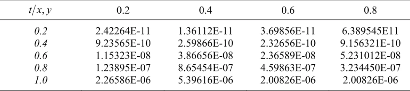
Table 1: The following table shows absolute errorϕ₇ for variablesx, and y t varies from 0.2 to 1.0 for Example 3.1.

y x

t , 0.2 0.4 0.6 0.8

0.2 0.4 0.6 0.8 1.0

2.42264E-11 9.23565E-10 1.15323E-08 1.23895E-07 2.26586E-06

1.36112E-11 2.59866E-10 3.86656E-08 8.65454E-07 5.39616E-06

3.69856E-11 2.32656E-10 2.36589E-08 4.59863E-07 2.00826E-06

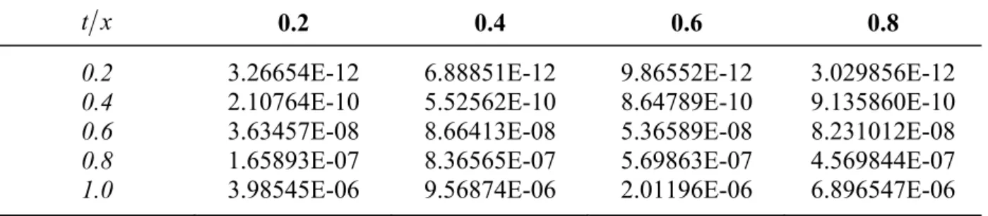
Table 2: The following table shows absolute error ϕ₈ for variable xand t varies from 0.2 to 1.0 for Example 3.2.

x

t 0.2 0.4 0.6 0.8

0.2 0.4 0.6 0.8 1.0

3.26654E-12 2.10764E-10 3.63457E-08 1.65893E-07 3.98545E-06

6.88851E-12 5.52562E-10 8.66413E-08 8.36565E-07 9.56874E-06

9.86552E-12 8.64789E-10 5.36589E-08 5.69863E-07 2.01196E-06

3.029856E-12 9.135860E-10 8.231012E-08 4.569844E-07 6.896547E-06

Table 3: The following table shows absolute error ϕ₁₀ for variable xand t varies from 0.2 to 1.0 for Example 3.3.

x

t 0.2 0.4 0.6 0.8

0.2 0.4 0.6 0.8 1.0

0.000000000 0.000000000 0.000000000 2.86954E-17 1.89658E-15

0.000000000 0.000000000 0.000000000 8.69872E-17 2.56856E-15

0.000000000 0.000000000 0.000000000 5.92313E-17 5.96845E-15

0.000000000 0.000000000 0.000000000 8.50096E-17 1.00236E-17

5 Figures

1 1.02 1.04 1.06 1.08 1.1 1.12 1.14 1.16 1.18

1 2 3 4 5 6 7 8

HPM Exact

t u

0 0.5 1 1.5 2 2.5 3 3.5 4

1 2 3 4 5 6

HPM Exact

t u

Figure 2: Comparison of exact solution and HPM solution of Example 3.2.

-5 -4 -3 -2 -1 0 1 2 3 4 5

1 2 3 4 5 6

HPM Exact u

t

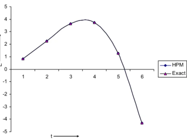
Figure 3: Comparison of exact solution and HPM solution of Example 3.3.

0.00E+00 1.00E-06 2.00E-06 3.00E-06 4.00E-06 5.00E-06 6.00E-06 7.00E-06 8.00E-06 9.00E-06 1.00E-05

0.5 0.7 0.9

t

0.00E+00 2.00E-06 4.00E-06 6.00E-06 8.00E-06 1.00E-05

0 0.2 0.4 0.6 0.8 1

t

Figure 5: Errors of Example 3.2 from various values of t =0 to t =1.

0

0.1

0.2 0

0.025 0.05

0.075 0.1

0 0.05

0.1

0

0.1

0.2

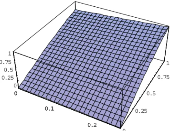
Figure 6:Exact solution graph of Example 3.1 for x=0 to x=1.

0

0.1

0.2 0

0.25 0.5

0.75 1

0 0.25

0.5 0.75

1

0

0.1

0.2

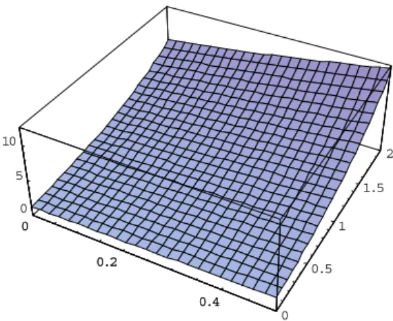
Figure 7: Approximate solution graph of Example 3.1 up to fifth approximation for x=0 to

0

0.2

0.4 0

0.25 0.5

0.75 1

1 2 3 4

0

0.2

0.4

Figure 8: Exact solution graph of Example 3.2 for x=0 to x=0.5.

0

0.2

0.4 0

0.5 1

1.5 2

0 5 10

0

0.2

0.4

Figure 9: Approximate solution graph of Example 3.2 up to fifth approximation for x=0 to

. 5 . 0 = x

0

0.1

0.2 0

5 10

15

-1 0 1

0

0.1

0.2

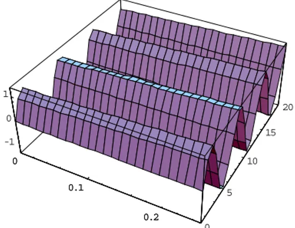
Figure 10:Approximate solution graph of Example 3.1 up to fifth approximation for t =0 to

0

0.1

0.2 0

5 10

15 20

-1 0 1

0

0.1

0.2

Figure 11: Approximate solution graph of Example 3.2 up to fifth approximation for t =0 to

. 20 = t

6 Conclusions

In this paper, the HPM has been successfully employed to obtain the approximate analytical solutions of the nonlinear wave-like equations with variable coefficients. In Examples 1-3 we observe that HPM solutions are more accurate than the ADM. Figs. 1 to 11 show that the solutions obtained by HPM are much closer to the exact solution for various values of time parameter. Table 1 to 3 denotes the less error for the solution obtained by HPM and exact solution. HPM avoids the difficulties arising in finding the Adomain polynomials. In addition, the calculations involved in HPM are very simple and straight forward. It is shown that the HPM is a promising tool for both linear and nonlinear partial differential equations. Mathematica 5.0 has been used for numerical computations in this paper.

References

Abbasbandy, S. (2007): Application of He's homotopy perturbation method to functional integral equations. Chaos Solitons Fractals 31, pp. 1243–1247.

Belendez, A., Pascual, C., Ortuno, M., Gallego, S. and Neipp, C. (2007): Application of

modified He's homotopy perturbation method to obtain higher order approximations of a x13 force nonlinear oscillator. Physics Letters A 371, pp. 421–426.

Belendez, A., Pascual, C., Belendez, T. and Hernandez, A. (2009a): Solution for an antisymmetric quadratic nonlinear oscillator by a modified He's homotopy perturbation method. Nonlinear Analysis RWA 10 (1), pp. 416–427.

Belendez, A., Pascual, C., Ortuno, M., Belendez, T. and Gallego, S. (2009b): Application of modified He's homotopy perturbation method to obtain higher order approximations to a nonlinear oscillator with discontinuities. Nonlinear Analysis RWA 10 (2), pp. 601–610.

Ganji, D. D. and Sadighi, A. (2006): Application of He's homotopy perturbation method to nonlinear coupled system of reaction-diffusion equations. International Journal of Nonlinear Sciences and Numerical Simulation 7, pp. 411–418.

Ghasemi, M., Tavassoli, M. and Babolian, E. (2007): Numerical solutions of the nonlinear Voltera-Fredholm integral equations by using homotopy perturbation method. Applied Mathematics and Computation 188, pp. 446–449.

Ghoreishi, M., Ismail, A. I. B. and Ali, N. H. M. (2010): Adomain decomposition method for nonlinear wave-like equation with variable coefficients. Applied Mathematical Sciences 4, pp. 2431–2444.

Gupta, S., Singh, J. and Kumar, D. (2013): Applications of homotopy perturbation transform method for solving time-dependent functional differential equations. International Journal of Nonlinear Science 16(1), pp. 37–49.

He, J. H. (1999): Homotopy perturbation techniques. Computer Methods in Applied Mechanics and Engineering 178, pp. 257–262.

He, J. H. (2000a): A review on some new recently developed nonlinear analytical techniques. International Journal of Nonlinear Sciences and Numerical Simulation 1(1), pp. 51–70.

He, J. H. (2000b): A coupling of homotopy technique and perturbation technique for nonlinear problems. International Journal of Nonlinear Mechanics 35(1) (2000), pp. 37–43.

He, J. H. (2003): Homotopy perturbation method: a new nonlinear analytical technique. Applied Mathematics and Computation 135, pp. 73–79.

Mehrabinezhad, M. and Saberi-Nadjafi, J. (2010): Application of He's homotopy perturbation method to linear programming problem, International Journal of Computer Mathematics 88 (2), pp. 341–347.

Momani, S. and Odibat, Z. (2007): Homotopy perturbation method for nonlinear partial differential equations of fractional order. Physics Letters A 365, pp. 345–350.

Odibat, Z. and Momani, S. (2008): Modified homotopy perturbation method: Application to Riccati differential equation. Chaos Solitons Fractals 36, pp. 167–174.

Ozis, T. and Yildirim, A. (2007a): A comparative study of He's homotopy perturbation method for determining frequency-amplitude relation of a nonlinear oscillators with discontinuity. International Journal of Nonlinear Science and Numerical Simulation 8 (2), pp. 243–248.

Ozis, T. and Yildirim, A. (2007b): Travelling wave solution of KdV equation using He' homotopy perturbation method. International Journal of Nonlinear Science and Numerical Simulation 8, pp. 239–242.

Rafei, M. and Ganji, D. D. (2006): Explicit solutions of Helmholtz equation and fifth-order KdV equation using homotopy perturbation method. International Journal of Nonlinear Sciences and Numerical Simulation 7, pp. 321–328.

Rafei, M., Ganji, D. D. and Daniali, D. (2007): Solution of epidemic model by homotopy perturbation method. Applied Mathematics and Computation 187, pp. 1056–1062.

Shanmugarajan, A., Alwarappan, S., Somasundaram, S. and Lakshmanan, R. (2011): Analytic solution of amperometric enzymatic reaction based on homotopy perturbation method. Electrochimica Acta 56 (9), pp. 3345–3352.

Siddique, A. M., Mahmood, R. and Ghori, Q. K. (2006): homotopy perturbation method for thin film flow of a fourth grade fluid down an inclined plane. Physics Letters A 352 (4–5), pp. 404–410.

Singh, J., Kumar D. and Kilicman, A. (2013): Homotopy perturbation method for fractional gas dynamics equation using sumudu transform. Abstract and Applied Analysis 2013, Article ID 934060, 8 pages.